Structure of Passive Circumstellar Disks: Beyond the Two-Temperature Approximation.

Abstract

Structure and spectral energy distributions (SEDs) of externally irradiated circumstellar disks are often computed on the basis of the two-temperature model of Chiang & Goldreich. We refine these calculations by using a more realistic temperature profile which is continuous at all optical depths and thus goes beyond the two-temperature model. It is based on the approximate solution of the radiation transfer in the disk obtained from the frequency-integrated moment equations in the Eddington approximation. We come up with a simple procedure (“constant $g_{z}$ approximation”) for treating the vertical structure of the disk in regions where its optical depth to stellar radiation is high. This allows us to obtain expressions for the vertical profiles of density and pressure at every point in the disk and to determine the shape of its surface. Armed with these analytical results we calculate the full radial structure of the disk and demonstrate that it favorably agrees with the results of direct numerical calculations. We also describe a simple and efficient way of the SED calculation based on our adopted temperature profile. Resulting spectra provide very good match (especially at short wavelengths) to the results of more detailed (but also more time-consuming) SED calculations solving the full frequency- and angle-dependent radiation transfer within the disk.

1. Introduction

Protoplanetary disks around T Tauri stars (stellar mass $M_{\star}\lesssim 2~{}M_{\odot}$) as well as the disks around more massive Herbig Ae/Be stars ($M_{\star}\gtrsim 2~{}M_{\odot}$) belong to the class of circumstellar disks that are strongly affected by the radiation of their central stars. Irradiation modifies both the vertical structure of the disk and the radial dependence of disk properties. As a result, observational signatures of centrally irradiated discs are quite different from those of the conventional viscously heated $\alpha$-disks (Shakura & Sunyaev 1972).

Kenyon & Hartmann (1987) have pointed out that the observed infrared spectra of protoplanetary disks can be understood as resulting from passive reprocessing of the stellar radiation assuming that disk surfaces have flared geometry. Later Chiang & Goldreich (1997; hereafter CG97) have analytically derived hydrostatic, radiative equilibrium models of disks around T Tauri stars. Their calculation was based on a two-temperature approximation for the disk thermal structure in which the outer “superheated” layer has been assumed isothermal at the temperature characteristic for dust grains directly illuminated by unattenuated stellar radiation. The isothermal midplane region was found to have lower temperature set by the balance between the oblique stellar illumination of the disk surface and the isotropic infrared emission of the disk interior. The success of this simple model has led to its wide acceptance for interpreting the observations of circumstellar disks.

The goal of this paper is to improve our understanding of the circumstellar disk structure by going beyond the simple two-temperature approximation of CG97. Calvet et al. (1991; hereafter C91) have studied the vertical radiative transfer within irradiated dusty circumstellar disks and obtained approximate analytical expression for the vertical temperature profile which is superior to the two-temperature approximation of CG97. In this work we employ this temperature distribution, which is reviewed in detail in §2, to calculate the disk structure and spectrum. Under certain conditions it is possible to derive approximate analytical solutions for the vertical disk structure as demonstrated in §3. This allows us to efficiently compute the radial dependence of various disk properties in §4 and to compare them with purely numerical solutions. Finally, in §5 we demonstrate how the use of the realistic temperature profile of C91 improves the calculation of the spectral energy distribution (SED) of circumstellar disks.

Throughout this study we assume the major heating source of the disk to be the radiation of the central star of mass $M_{\star}$, having radius $R_{\star}$ and effective temperature $T_{\star}$. Viscous heating is considered subdominant. Circumstellar disk extending from $R_{in}$ to $R_{out}$ is assumed to be geometrically thin thus allowing us to neglect radial transport of radiation. This simplifies radiative transfer within the disk and reduces it to a one-dimensional problem. Surface density of the disk $\Sigma_{0}$ varies as

$$\Sigma_{0}(a)=\Sigma_{\star}\left(\frac{R_{\star}}{a}\right)^{\delta},$$ (1)

where $a$ is the distance from the central star and $\Sigma_{\star}\equiv\Sigma(R_{\star})$. We use $\delta=1$ in our calculations. Our results will be illustrated using three fiducial models of circumstellar disks around Herbig Ae/Be star, T Tauri star, and a brown dwarf, analogous to those adopted by Dullemond & Natta (2003; hereafter DN03). Properties of these models are summarized in Table 1 ($\Sigma_{1}\equiv\Sigma_{\star}(R_{\star}/1~{}\mbox{AU})^{\delta}$ is the value of $\Sigma_{0}$ at $1$ AU).

2. Thermal structure.

To describe the transfer of stellar radiation with blackbody temperature $T_{\star}$ within the disk we introduce optical depth $\tau_{\star}(z)$ ($z$ is the altitude above the disk midplane) which is calculated along the radial direction from the star. Following conventional wisdom we approximate $\tau_{\star}$ as

$$\tau_{\star}(z)\approx\alpha^{-1}\int\limits_{z}^{\infty}\kappa_{P}(T_{\star})\rho(z)dz=\alpha^{-1}\kappa_{P}(T_{\star})\Sigma(z),$$ (2)

where $\rho(z)$ is the local gas density, $\Sigma(z)\equiv\int_{z}^{\infty}\rho(z)dz$ is the disk surface density above a given $z$, $\kappa_{P}(T)$ is the Planck mean opacity at temperature $T$, and $\alpha$ is the flaring angle ($\pi/2-\alpha$ is the angle between the normal to the disk surface and the radial direction). In the thin disk approximation

$$\alpha\approx\eta\frac{R_{\star}}{a}+a\frac{d}{da}\left(\frac{H_{1}}{a}\right),$$ (3)

where $H_{1}(a)$ is the altitude of the disk surface defined as a surface at which $\tau_{\star}(a,H_{1})=1$ and $\eta\approx 0.4$ is constant (Kenyon & Hartmann 1987; CG97). There are two regimes of irradiation: “lamp-post” illumination when $R_{\star}\gtrsim H_{1}$ and

$$\alpha\approx\eta\frac{R_{\star}}{a},$$ (4)

and “point-source” illumination when $R_{\star}\lesssim H_{1}$ and

$$\alpha\approx a\frac{d}{da}\left(\frac{H_{1}}{a}\right).$$ (5)

In the first case the geometry of illumination is determined by the finite size of the source, while in the second it is the self-adjustment of the disk surface geometry that sets the illumination angle. Apparently, disk must be flared in the latter case, i.e. $d(H_{1}/a)/da>0$.

Figure 1.— Opacity $\kappa_{\nu}$ (solid curve) adopted in this paper as a function of frequency $\nu$ (lower axis) and Planck opacity $\kappa_{P}$ (dashed curve) computed based on this $\kappa_{\nu}$ as a function of temperature $T=h\nu/k$ (upper axis).

Dust grains are the major opacity source in circumstellar disks except their central regions where high temperature leads to dust sublimation. To compute $\kappa_{P}(T)$ we use the frequency-dependent opacity $\kappa_{\nu}$ characteristic of $0.1$ $\mu$m silicate grains (Draine & Lee 1984) with no scattering (the same as $\kappa_{\nu}$ used by DN03, to facilitate subsequent comparison with their results). Both $\kappa_{P}(T)$ and $\kappa_{\nu}$ used in this study are shown in Figure 1.

At low temperatures ($T\lesssim 10^{2}$ K) $\kappa_{P}$ behaves as a power law of $T$. Motivated by this, in deriving our analytical results we will frequently use the “local power law opacity” approximation to $\kappa_{P}(T)$. It is defined as the best power law fit to the actual run of $\kappa_{P}(T)$ in the temperature range relevant at a given distance from the star $a$:

$$\kappa_{P}(T)\approx\kappa_{0}(a)T^{\beta(a)},$$ (6)

where parameters $\kappa_{0}$ and $\beta$ are functions of $a$. This simplified approach shows very good agreement with numerical calculations using full $\kappa_{P}(T)$, see §4.

Calvet et al. (C91) have derived approximate temperature structure of centrally irradiated accretion disk heated from inside by viscous dissipation. Their result is based on the assumption that disk is optically thick to its own radiation with opacity independent of temperature. For simplicity, in this study we neglect radiation scattering by dust and viscous heating. At the same time, the assumption of a geometrically thin disk allows us to generalize C91 result for an arbitrary dependence of $\kappa_{P}$ on $T$. Simple calculation in the spirit of C91 results in the following implicit expression for $T$:

$$T^{4}(z)=\phi T_{\star}^{4}\left(\frac{R_{\star}}{a}\right)^{2}\left[\frac{\alpha}{2}\frac{\psi_{ex}}{\psi_{sh}}+\frac{q(T)}{4}e^{-\tau_{\star}(z)}\right].$$ (7)

Here $q(T)=\kappa_{P}(T_{\star})/\kappa_{P}(T)$ is a ratio of opacities at temperatures $T_{\star}$ and $T$, factor $\phi$ represents the fraction of the stellar surface visible from a given point of the disk surface, while $\tau_{\star}(z)$ and $\alpha$ are given by equations (2) & (3). If the inner edge of the disk is close to the stellar surface – an assumption that we adopt in this paper – then $\phi\approx 1/2$. Following Dullemond, Dominik & Natta (2001; hereafter DDN), we have introduced correction factors $\psi_{ex}\leq 1$ and $\psi_{sh}\leq 1$ to make this solution valid even when the disk is optically thin to the radiation of its outer layer and/or its interior [situations not allowed in the original optically thick solution of C91 which can be recovered from eq. (7) by setting $\psi_{ex}=\psi_{sh}=1$]. We provide details of the calculation of $\psi$-factors in Appendix A.

According to equation (7) the vertical extent of the disk can be split into two layers: the outer layer exposed to stellar radiation and the inner layer shielded from direct starlight (see Figure 2 for an illustration).

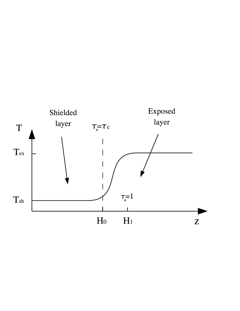
Figure 2.— Schematic illustration of the vertical thermal structure of irradiated disk adopted in this paper. See text for detailed explanations.

Dust within the exposed layer absorbs highly anisotropic stellar flux with blackbody temperature $T_{\star}$ and reradiates it isotropically at lower temperature. A half of the reradiated flux escapes while another half illuminates the interior of the disk. Temperature in the exposed layer varies vertically according to

$$T\approx T_{\star}\left(\frac{R_{\star}}{2a}\right)^{1/2}\left[\phi q(T)e^{-\tau_{\star}(z)}\right]^{1/4}$$ (8)

$$\approx T_{ex}(a)e^{-\tau_{\star}/(4+\beta)}.$$ (9)

where

$$T_{ex}(a)=T_{\star}\left[\phi q(T_{ex})\right]^{1/4}\left(\frac{R_{\star}}{2a}\right)^{1/2}$$ (10)

$$=T_{\star}\left(\frac{R_{\star}}{2a}\right)^{2/(4+\beta)}\phi^{1/(4+\beta)}.$$ (11)

Expressions (9) and (11) correspond to the case of the power law opacity (6). It follows from equation (8) that $T_{ex}$ is the temperature of the optically thin part of the disk ($\tau_{\star}\ll 1$). Exposed layer corresponds to $\tau_{\star}\lesssim\tau_{c}$ where

$$\tau_{c}\equiv\ln\left[\frac{q(T_{sh})}{2\alpha}\frac{\psi_{sh}}{\psi_{ex}}\right].$$ (12)

We denote $H_{0}(a)\equiv z(\tau_{\star}=\tau_{c})$ the height at which optical depth $\tau_{\star}$ equals $\tau_{c}$.

Shielded layer lies below the exposed region at high optical depth, $\tau_{\star}\gtrsim\tau_{c}$. Within this layer disk material receives only the reprocessed radiation of the exposed layer since the direct stellar flux is almost entirely absorbed by the exposed layer. Shielded region is isothermal with temperature

$$T_{sh}(a)=T_{\star}\left(\frac{\phi\alpha}{2}\frac{\psi_{ex}}{\psi_{sh}}\right)^{1/4}\left(\frac{R_{\star}}{a}\right)^{1/2},~{}~{}~{}\tau_{\star}\gtrsim\tau_{c}.$$ (13)

Equation (13) results from balancing the incoming flux of the reprocessed radiation with the energy loss from the shielded layer. Factors $\psi_{sh}$ and $\psi_{ex}$ in equations (12) and (13) accounting for the possibility of optically thin disk are set by $T_{sh}$ and $T_{ex}$, see equations (A2) and (A4).

Temperature profile (7) should be compared with the temperature structure adopted by CG97:

$$T = T_{ex},~{}~{}~{}~{}~{}\tau_{\star}<1,$$ (14)

$$= T_{sh},~{}~{}~{}~{}~{}\tau_{\star}\geq 1.$$

Equation (7) provides a better match for the real thermal structure of the exposed layer as it does not feature an unphysical temperature jump at some optical depth.

3. Vertical structure.

Hydrostatic equilibrium in $z$-direction is described by

$$\frac{dP}{dz}=-\Omega^{2}z\rho,$$ (15)

where $P$ is the gas pressure and $\Omega\equiv(GM_{\star}/a^{3})^{1/2}$ is the local angular frequency. Within the isothermal shielded layer ($z\lesssim H_{0}$) this equation yields

$$\frac{\rho(a,z)}{\rho_{0}(a)}=\frac{P(a,z)}{P_{0}(a)}=\exp\left[-\frac{z^{2}}{2h_{sh}^{2}(a)}\right],$$ (16)

where $h_{sh}\equiv\Omega^{-1}(k_{B}T_{sh}/\mu)^{1/2}$ is the isothermal scaleheight of the disk in the shielded region, and $\rho_{0}$ and $P_{0}$ are the midplane values of gas density and pressure. Because of the exponential decay of $\rho$ with $z$ shielded region contains most of the surface density $\Sigma_{0}(a)$ of the disk (if $H_{0}\gtrsim h_{sh}$) which implies that

$$\rho_{0}(a)\approx(2\pi)^{-1/2}\frac{\Sigma_{0}(a)}{h_{sh}},~{}~{}~{}P_{0}=\frac{\rho_{0}}{\mu}k_{B}T_{sh}.$$ (17)

3.1. Constant $g_{z}$ approximation.

Exposed region is not isothermal when $\tau_{\star}\sim 1$ but we can still understand its vertical structure by introducing the so-called constant $g_{z}$ approximation. This approximation makes use of the fact that gas density in the disk decreases very rapidly with increasing $z$, see e.g. (16). As a result, when considering the hydrostatic equilibrium, we can to zeroth order neglect the variation of the vertical acceleration $g_{z}=\Omega^{2}z$ compared to the change of $\rho$ with $z$ in equation (15).

In particular, for the determination of the disk structure near its surface we can set $z\approx H_{1}$ which allows us to integrate equation (15) over $z$. We find that $P(z)\approx\Omega^{2}H_{1}\Sigma(z)$ and using definition (2) obtain the following relation between $P$ and $\tau_{\star}(z)$:

$$P(\tau_{\star})\approx\alpha\frac{\Omega^{2}H_{1}}{\kappa_{P}(T_{\star})}\tau_{\star}.$$ (18)

Substituting this into equation (15) one finds

$$\frac{1}{\tau_{\star}}\frac{d\tau_{\star}}{dz}\approx-z\frac{\Omega^{2}\mu}{k_{B}T(\tau_{\star})}.$$ (19)

In the shielded region below $H_{0}$ (we assume that $H_{0}\sim H_{1}$ which is verified below) $T(\tau_{\star})\approx T_{sh}$ and equation (19) yields

$$\frac{z^{2}}{2h_{sh}^{2}}\approx\ln\left[\frac{P_{0}\kappa(T_{\star})}{\alpha\Omega^{2}H_{1}}\right]-\ln\tau_{\star}.$$ (20)

Integration constant is fixed in equation (20) with the aid of equation (18) by noticing that in the shielded region solution (20) must reduce to (16). Substituting $\tau_{\star}=\tau_{c}$ into equation (20) one obtains the height of the boundary between the exposed and shielded layers $H_{0}$:

$$H_{0}=\lambda h_{sh},~{}~{}~{}~{}\lambda\equiv\left(2\ln\Lambda\right)^{1/2},$$ (21)

$$\Lambda\equiv\frac{P_{0}\kappa(T_{\star})}{\alpha\tau_{c}\Omega^{2}H_{0}}=\frac{\Sigma_{0}\kappa(T_{\star})}{\sqrt{2\pi}\alpha\tau_{c}\lambda}.$$ (22)

Our use of $H_{0}$ instead of $H_{1}$ in the definition of $\Lambda$ improves the accuracy of (22).

Structure of the exposed region will be determined under the assumption of the “local power law opacity” approximation (6) which allows us to use equation (9). When integrating equation (19) for $z>H_{0}$ we can split the integral into two parts: $\int^{\tau_{\star}}=\int^{\tau_{c}}+\int^{\tau_{\star}}_{\tau_{c}}$. In the first integral we set $T(\tau_{\star})=T_{sh}$ which reduces it to equation (20), while in the second we use $T(\tau_{\star})$ given by equation (9). As a result, for $z\gtrsim H_{0}$ one finds

$$z^{2}\approx H_{0}^{2}-2h_{ex}^{2}\left[\rm{Ei}\left(-\frac{\tau_{\star}}{4+\beta}\right)-\rm{Ei}\left(-\frac{\tau_{c}}{4+\beta}\right)\right],$$ (23)

where $h_{ex}\equiv\Omega^{-1}(k_{B}T_{ex}/\mu)^{1/2}$ is the disk scale height corresponding to temperature $T_{ex}$ and ${\rm Ei}(x)\equiv-\int^{\infty}_{-x}t^{-1}e^{-t}dt$ is exponential integral (Gradshtein & Ryzhik 2000).

Equation (23) allows us to determine the position of the disk surface:

$$H_{1}^{2}\approx H_{0}^{2}+\chi^{2}h_{ex}^{2},$$ (24)

$$\chi^{2}\equiv-2\left[\rm{Ei}\left(-\frac{1}{4+\beta}\right)-\rm{Ei}\left(-\frac{\tau_{c}}{4+\beta}\right)\right]>0,$$ (25)

where for all practical purposes factor $\chi\sim 1$ can be considered almost constant – although $\tau_{c}\gtrsim 1$ is a function of $a$, the corresponding contribution in (25) is small compared to the leading term $\rm{Ei}(-1/(4+\beta))$. One can see that $H_{1}\sim H_{0}$ unless $\lambda\lesssim\chi T_{ex}/T_{sh}$ (which can only be realized when the constant $g_{z}$ approximation breaks down, see §4.1 and Figures 3-5). Asymptotically

$${\rm Ei}(-x) \simeq -\frac{e^{-x}}{x}\left[1+O(x^{-1})\right],~{}~{}~{}x\gg 1,$$ (26)

$$\simeq {\bf C}+\ln(x)+O(x),~{}~{}~{}~{}~{}~{}x\ll 1,$$

(Gradshtein & Ryzhik 2000) where ${\bf C}\approx 0.5772$ is the Euler constant. These limiting forms suggest that

$$z^{2}\approx H_{0}^{2}+2(4+\beta)h_{ex}^{2}\frac{e^{-\tau_{\star}/(4+\beta)}}{\tau_{\star}},$$ (27)

for $1\lesssim\tau_{\star}\lesssim\tau_{c}$ ($H_{0}\lesssim z\lesssim H_{1}$) while

$$\tau_{\star}(z)\approx(4+\beta)e^{-{\bf C}}\exp\left(-\frac{z^{2}-H_{0}^{2}}{2h_{ex}^{2}}\right),$$ (28)

$$\frac{P(z)}{P_{0}}\approx\frac{\rho(z)}{\rho_{0}}$$

$$\approx\frac{(4+\beta)e^{-{\bf C}}}{\tau_{c}}\exp\left(-\frac{z^{2}-H_{0}^{2}}{2h_{ex}^{2}}-\frac{H_{0}^{2}}{2h_{sh}^{2}}\right),$$ (29)

for $\tau_{\star}\lesssim 1$ ($z\gtrsim H_{1}$). The dependence (28) is somewhat unexpected given that the exposed region above $H_{1}$ is virtually isothermal at temperature $T_{ex}$. Apparently, this is an artifact of our adopted constant $g_{z}$ approximation. At the same time $P(z)$ and $\rho(z)$ given by (29) are in accord with the isothermality of this part of the disk which is to some extent coincidental.

Equations (21)-(29) fully determine the vertical hydrostatic structure of the disk as well as the positions of $H_{0}(a)$ and $H_{1}(a)$ through the parameters of the disk and the star.

3.2. Comparison with the two-temperature approximation.

It is instructive to compare the results of the previous section with the disk structure according to CG97. Their model exhibits discontinuous jump of temperature at $\tau_{\star}=1$ and assumes upper disk layer ($\tau_{\star}<1$) to be fully isothermal, see equation (14). This layer (“superheated dust layer” in their nomenclature) plays the role of our exposed region, while the underlying region ($\tau_{\star}>1$) should be identified with our shielded layer. In both layers vertical profile of pressure is Gaussian and $\rho$ is discontinuous across the boundary defined by $\tau_{\star}=1$ (while $P$ is continuous there). Apparently, $H_{0}=H_{1}$ in the CG97 model; applying constant $g_{z}$ approximation with their temperature structure (14) one finds $H_{1}$ to be given by equation (21) but with $\Lambda$ replaced by

$$\Lambda_{\rm CG}=\frac{\Sigma_{0}\kappa(T_{\star})}{\sqrt{2\pi}\alpha\lambda_{\rm CG}}.$$ (30)

The position of the disk surface computed in the two-temperature approximation deviates from that given by equation (24). Difference is not very significant in the inner disk where $\lambda^{2}h_{sh}^{2}\gg\chi^{2}h_{ex}^{2}$. However, at intermediate radii this is no longer valid and the two-temperature model underestimates $H_{1}$ compared to our more accurate expression (24).

4. Radial properties of irradiated disks.

Based on analytical results obtained in the previous section we can provide a complete description of the irradiated disk structure. This requires the determination of $T_{sh}(a)$ which can be done by substituting $H_{1}(a)$ given by the expression (24) into (3), plugging $\alpha$ into (13) and solving the resultant differential equation for $T_{sh}(a)$.

Figure 3.— Comparison between the semi-analytical (constant $g_{z}$ approximation) and numerical approaches to computing the disk structure in Model I. (a) Position of the disk surface $H_{1}(a)/a$ calculated using eq. (24) (solid curve) and numerically with the full treatment of the vertical hydrostatic equilibrium (short-dashed curve). Also shown are the semi-analytical results for $H_{0}(a)/a$ (dot-dashed line), $h_{sh}(a)/a$ (long-dashed line), and the ratio $h_{sh}/H_{0}=\lambda^{-1}$ (dotted line). (b) Midplane temperature $T_{sh}(a)$ computed semi-analytically (solid curve) and numerically (short-dashed curve). Two methods give virtually identical results in this case. Dotted line represents $T_{ex}(a)$. (c) Flaring angle $\alpha(a)$ obtained semi-analytically (solid curve) and numerically (short-dashed curve).

Analytical expressions for $T_{sh}(a)$ can be obtained for optically thick disks ($\psi_{ex}=\psi_{sh}=1$) which either (1) are illuminated in the lamp-post regime or (2) experience point-like illumination and have $\lambda=H_{0}/h_{sh}$ of the order of several (typically $\gtrsim 3$). In the latter case one can neglect in equation (24) term $\chi h_{ex}$ compared to $\lambda h_{sh}$, which, coupled with the weak sensitivity of $\lambda$ to $a$, leads to $H_{1}\propto h_{sh}$. This assumption should be valid in the inner, dense parts of circumstellar disks. Analytical results for these two cases are summarized in Appendix B. In particular, one finds that $H_{1}\propto a^{9/8}$ for lamp-post illumination and $H_{1}\propto a^{9/7}$ for point-like illumination, i.e. in both cases disk surface is flared. In a more general case we find the behavior of $T_{sh}(a)$ by solving the system of equations (3), (13), and (24) numerically.

To test the validity of the constant $g_{z}$ approximation we additionally compute disk structure without analytical approximations of §3.1, with the only assumption that the temperature profile is given by equation (7). In this approach at every radius we calculate vertical disk structure numerically with equations (7) and (15), instead of using the results of §3.1. The value of $H_{1}$ obtained in this fashion (instead of using equation [24]) is then used in equation (3) to reconstruct the radial disk profile. This approach uses the detailed opacity description $\kappa_{P}(T)$ shown in Figure 1, while our semi-analytical procedure calculates disk structure assuming local power law opacity fit (6) to the curve of $\kappa_{P}(T)$. Some details of the numerical disk structure calculation can be found in Appendix C.

Figure 4.— Same as Figure 3 but for Model II.

In Figures 3-5 we present our results for the three disk models listed in Table 1. We compare the behaviors of $H_{1}(a)$, $T_{sh}(a)$, and $\alpha(a)$ found semi-analytically and numerically. One can see that the theory based on the constant $g_{z}$ approximation predicts $H_{1}(a)$ quite well – the discrepancy with the numerical result at the level of $\sim 10\%$ appears only in the outermost parts of the disk. The same is true for $T_{sh}(a)$. Flaring angle $\alpha$ is a more sensitive probe of the difference between the two approaches as it involves a derivative of $H_{1}(a)$. In the outer regions of disks in models II and III semi-analytical $\alpha(a)$ diverges significantly from the numerical solution. This is the result of the lower optical depth in these models compared to the model I, which affects the validity of the constant $g_{z}$ approximation, see §4.1.

Nevertheless, at small and intermediate $a$ the overall agreement between the two methods of the disk structure calculation is very good. For illustration, in Figure 6 we present the comparison between the vertical profiles of $T$, $P$, $\rho$, and $\tau$ obtained by both methods at $a=10$ AU in Model II. Despite the fact that at this location constant $g_{z}$ approximation is already close to the limit of its validity (see Figure 4) the agreement in the vertical structure of $P$, $\rho$, and $T$ is quite remarkable. The constant $g_{z}$ approximation fails only for $\tau_{\star}(z)$ which was expected, see discussion after equation (29).

4.1. Validity of the constant $g_{z}$ approximation.

Constant $g_{z}$ approximation should work well when $H_{0},H_{1}\gtrsim h_{sh}$ since in this case the decay of $P$ and $\rho$ with height is well represented by the tail of the Gaussian profile at $z\sim H_{0},H_{1}$. As a result, at this height $\rho$ varies with $z$ much faster than $g_{z}$ and constant $g_{z}$ limit works well. Based on this reasoning, we can tentatively suggest $H_{0}\gtrsim 2h_{sh}$ as an approximate criterion for the validity of this approximation.

Figure 5.— Same as Figure 3 but for Model III.

This conclusion is confirmed by examination of Figures 3-5 which demonstrate that the relative difference between the values of $\alpha$ computed with and without constant $g_{z}$ approximation starts to exceed $10\%$ when the ratio $H_{0}/h_{sh}=\lambda$ drops below $\approx 2.5$. Using definition (21) we can then claim this approximation to be accurate (at the level of $\sim 10\%$) whenever $\Lambda\gtrsim 20$ or

$$\kappa_{P}(T_{\star})\Sigma_{0}\gtrsim 10,$$ (31)

where we have taken into account that in our models $\sqrt{2\pi}\alpha\tau_{c}\approx 0.5$ at the limit of applicability. This condition is accurate only in the order of magnitude as the exact factor in its right hand side is exponentially sensitive to the uncertainties in $\lambda$. Despite this, in practical situations one may still use condition (31) as a rough proxy for checking whether the constant $g_{z}$ approximation can be relied upon.

Figure 6.— Vertical structure of the disk in Model II at $a=10$ AU. Results for $\rho(z)$ (a), $\tau(z)$ (b), $T(z)$ (c), and $P(z)$ (d) are shown. Solid curves represent fully numerical results while dashed curves represent results obtained using constant $g_{z}$ approximation. Locations of $h_{sh}$, $H_{0}$, and $H_{1}$ are marked on each panel by dashed lines.

5. Spectral energy distribution.

Figure 7.— Spectral energy distribution of a disk annulus around Herbig Ae/Be star ($T_{\star}=10^{4}$ K, $R_{\star}=2~{}R_{\odot}$, $M_{\star}=2~{}M_{\odot}$). Annulus is placed at $a=1$ AU, it has a width $\Delta a=0.01$ AU, flaring angle $\alpha=0.05$, and vertical optical depth $\tau=10$ at $550$ nm. Dashed line shows SED calculated according to equations (32) and (34), solid line represents SED calculated using full frequency- and angle-dependent radiation transfer (DN03), while dotted line is SED computed in the framework of the two-temperature approximation (CG97).

In this section we calculate disk SED using our adopted temperature profile (7), and then compare the outcome with the results of other approaches.

In our case SED is produced by emission of both shielded and exposed layers. The contribution of the former per unit surface area of the disk $dF_{\nu}^{sh}(a)/dS$ is given simply by (see DDN)

$$\frac{dF_{\nu}^{sh}(a)}{dS} = 2\pi\cos i\left\{1-\exp\left[-\frac{\Sigma_{0}(a)\kappa_{\nu}}{\cos i}\right]\right\}$$ (32)

$$\times B_{\nu}\left[T_{sh}(a)\right],$$

where $i$ is the disk inclination (we assume disk thickness to be so small that all elements of its surface can be characterized by a single value of inclination), $B_{\nu}(T)$ is a Planck function, and the factor in parentheses accounts for the possibility of the disk being optically thin at a given frequency $\nu$.

Exposed layer is always optically thin to its own radiation and its contribution to the SED is given by

$$\frac{dF_{\nu}^{ex}(a)}{dS} = 2\pi\left\{1+\exp\left[-\frac{\Sigma_{0}(a)\kappa_{\nu}}{\cos i}\right]\right\}$$ (33)

$$\times \int\limits_{0}^{\tau_{\nu,c}}B_{\nu}\left[T(a,\tau_{\star})\right]d\tau_{\nu},$$

where $\tau_{\nu}=\alpha\tau_{\star}\kappa_{\nu}/\kappa_{P}(T_{\star})$ is the optical depth at frequency $\nu$ along the disk normal, $T(a,\tau_{\star})$ is given by (10), and the factor in parentheses accounts for the contribution of the exposed layer on the other side of the disk when the shielded layer is optically thin at frequency $\nu$. Here $\tau_{\nu,c}=\alpha\tau_{c}\kappa_{\nu}/\kappa_{P}(T_{\star})\ll 1$ is the value of $\tau_{\nu}$ at the boundary between the shielded and exposed layers.

Figure 8.— Same as Figure 7 but for annulus at $a=50$ AU from the star having width $\Delta a=0.5$ AU and vertical optical depth $\tau=300$ at $550$ nm.

Using equation (10) one can switch from integration over $d\tau_{\nu}$ to integration over $y\equiv h\nu/k_{B}T$ in the range $y_{0}<y<\infty$, where $y_{0}\equiv h\nu/k_{B}T_{ex}$. The upper limit $h\nu/k_{B}T_{sh}$ can be extended to $\infty$ since most of the exposed layer emissivity originates at temperatures $\sim T_{ex}$ corresponding to $y\sim y_{0}$. As a result, one obtains

$$\frac{dF_{\nu}^{ex}(a)}{dS}=2\pi\left\{1+\exp\left[-\frac{\Sigma_{0}(a)\kappa_{\nu}}{\cos i}\right]\right\}A_{\nu}(T_{ex}),$$ (34)

where

$$A_{\nu}(T_{ex}) = \alpha\frac{\kappa_{\nu}}{\kappa_{P}(T_{\star})}\int\limits_{0}^{T_{ex}}\frac{dT}{T}B_{\nu}(T)\psi(T)$$ (35)

$$= \alpha\frac{2h\nu^{3}}{c^{2}}\frac{\kappa_{\nu}}{\kappa_{P}(T_{\star})}\int\limits_{y_{0}}^{\infty}\frac{dy}{y}\frac{\psi\left(h\nu/ky\right)}{e^{y}-1},$$

is the emissivity of the exposed layer. Function $\psi(T)$ is defined as

$$\psi(T) \equiv 4+\frac{d\ln\kappa_{P}(T)}{d\ln T}$$ (36)

$$= \frac{\int_{0}^{\infty}B_{\nu}(T)\kappa_{\nu}\left(4+d\ln\kappa_{\nu}/d\ln\nu\right)d\nu}{\int_{0}^{\infty}B_{\nu}(T)\kappa_{\nu}d\nu}.$$

Equations (34)-(36) provide us with the method of calculation of the SED of the exposed layer that does not require an explicit solution of (7) to obtain $T(\tau_{\star})$ but at the same time fully accounts for the non-isothermal nature of the exposed layer.

Full emissivity is given by the sum of $dF_{\nu}^{sh}(a)/dS$ and $dF_{\nu}^{ex}(a)/dS$. In Figures 7-9 we display the SED produced by the thin disk annulus placed at different radii around different stars (their parameters can be found in figure captions), assuming a fixed value of the flaring angle $\alpha=0.05$ and inclination $i=0^{\circ}$ for all of them. This choice allows us to directly check our results against the calculations of DN03 who have made an exhaustive comparison between the two-temperature model and the full numerical treatment of the radiative and hydrostatic equilibrium of the disk, using both frequency- and angle-dependent radiation transfer in $z$-direction.

Figure 9.— Same as Figure 7 but for an annulus around T Tauri star ($T_{\star}=4000$ K, $R_{\star}=2~{}R_{\odot}$, $M_{\star}=0.5~{}R_{\odot}$). Annulus is placed at $a=0.1$ AU and has width $\Delta a=0.001$ AU and vertical optical depth $\tau=10$ at $550$ nm.

Figures 7-9 show that at short wavelengths our treatment (34)-(36) of the temperature structure of the exposed layer reproduces full numerical SED remarkably well, much better than the two-temperature approximation. This is not surprising since unlike our equation (10) the two-temperature model does not capture the smooth transition between $T_{ex}$ and $T_{sh}$ in the exposed layer and this affects its performance at high frequencies.

At longer wavelengths situation is more complicated. In particular cases represented in Figures 7 and 9 there is very nice agreement between our SED calculations and the numerical results of DN03 in the whole range of wavelengths. However, in the case displayed in Figure 8 situation is not so simple: both our approach and the two-temperature approximation give very similar results but deviate significantly from the SED computed by DN03 at $\lambda\sim 100$ $\mu$m. This has to do with the fact that at longer wavelengths disk spectrum becomes more sensitive to the details of the thermal structure of the shielded layer which is treated similarly by both our method and the two-temperature approach of CG97. However, it has been previously shown by Dullemond, van Zadelhoff & Natta (2002) that in some cases neither equation (7) nor (14) reproduce the temperature structure of the shielded layer accurately enough, and this causes discrepancies at long wavelengths in spectral calculations. Nevertheless, the much better agreement at short wavelengths obtained with our procedure at the expense of only slightly increased (compared to the two-temperature model) complexity justifies its practical use in various applications.

6. Discussion and Summary.

We have explored structure of the irradiated circumstellar disk based on a realistic temperature profile (7), which is more accurate than the two-temperature approximation of CG97. Our results on the disk SEDs presented in §5 persuasively demonstrate that this approach is superior to that of CG97 or DDN as it naturally reproduces the spectral behavior at short wavelengths without making any artificial assumptions.

This improvement is significant because of the recently emerged interest to the structure of the SED around $\lambda\sim 2$ $\mu$m. Many circumstellar disks exhibit excess emission in this band (Hillenbrand et al. 1992) which has been generally interpreted as the evidence for the existence of the dust sublimation region in the inner parts of these disks (DDN). Examination of Figures 7 & 9 reveals that the use of the two-temperature approximation can significantly overestimate the contribution of the disk to the total flux in this band. As a result, one would underestimate the amount of emission produced by the dust sublimation region and this can seriously affect the interpretation of the data. On the contrary, our approach reproduces realistic disk SEDs (obtained by DN03 using rather time-consuming procedure for solving full radiation transfer) very accurately at short wavelengths and, thus, can be relied upon when determining the emissivity of the dust sublimation region from the data. Note that our method of SED calculation based on equation (7) is no more computationally intensive than the two-temperature approximation of CG97 which is routinely used for analyzing protoplanetary disk spectra.

Another goal of this study was to introduce and test the constant $g_{z}$ approximation (§3.1) for treatment of the irradiated circumstellar disk structure. We have demonstrated by comparison with numerical results (4) that within its region of applicability [see equation (31)] this approximation works very well. Its use has allowed us to obtain analytical solutions for the vertical disk structure and to determine the position of the disk surface as a function of distance from the star rather accurately through the disk and stellar parameters. Improved description of the density and temperature structure of gas in the disk photosphere at $\tau_{\star}\sim\tau_{c}$ obtained in §3.1 allows one to improve the predictions of molecular line intensities compared to the two-temperature approximation [see Dullemond et al. (2002) for comparison of the line intensities obtained using full radiation transfer and its simplified representation given by equation (7)].

Finally, solutions presented in §3.1 allow fast and efficient exploration of the large phase space of circumstellar disk parameters when fitting disk SEDs. Their analytical nature will also be useful for treating more complicated problems, e.g. determining the structure of the dust sublimation region, ice lines, and so on.

Appendix A $\psi$-factors for optically thin disks.

Distant parts of the circumstellar disk where $\Sigma_{0}$ is small and temperature is low can be optically thin to the radiation of the shielded layer ($\Sigma_{0}\kappa_{P}(T_{sh})\lesssim 1$) and/or the exposed layer ($\Sigma_{0}\kappa_{P}(T_{ex})\lesssim 1$). To account for this possibility one introduces factor $\psi_{sh}<1$ defined as the ratio of the shielded layer emissivity to its value in the optically thick case. Factor $\psi_{ex}<1$ is defined as the fraction of radiation emitted by the exposed layer that gets absorbed by the shielded layer.

There are different ways of defining $\psi$-factors. In particular, Chiang et al. (2001) used simply

$$\psi_{sh}^{\rm C}(T_{sh})=1-\exp\left[-\Sigma_{0}\kappa_{P}(T_{sh})\right],~{}~{}~{}\psi_{ex}^{\rm C}(T_{ex})=1-\exp\left[-\Sigma_{0}\kappa_{P}(T_{ex})\right],$$ (A1)

while DDN suggested more accurate expressions for $\psi_{sh}$ and $\psi_{ex}$:

$$\psi_{sh}^{\rm DDN}(T_{sh})=\frac{\int_{0}^{\infty}B_{\nu}(T_{sh})\left[1-\exp\left(-\Sigma_{0}\kappa_{\nu}\right)\right]d\nu}{\sigma T_{sh}^{4}},$$ (A2)

$$\psi_{ex}^{\rm DDN}(T_{ex})=\frac{\int_{0}^{\infty}B_{\nu}(T_{ex})\kappa_{\nu}\left[1-\exp\left(-\Sigma_{0}\kappa_{\nu}\right)\right]d\nu}{\kappa_{P}(T_{ex})}.$$ (A3)

All of these expressions assume that corresponding layers of the disk emit pure blackbody radiation which is a reasonable assumption for the isothermal shielded layer (and so $\psi_{sh}^{\rm DDN}$ should be accurate). However, the temperature of the exposed layer varies quite dramatically when $1\lesssim\tau_{\star}\lesssim\tau_{c}$ and its spectrum must deviate from $B_{\nu}(T_{ex})$. For this reason, for $\psi_{ex}$ we use the following expression:

$$\psi_{ex}(T_{ex})=\frac{\int_{0}^{\infty}A_{\nu}(T_{ex})\left[1-\exp\left(-\Sigma_{0}\kappa_{\nu}\right)\right]d\nu}{\int_{0}^{\infty}A_{\nu}(T_{ex})d\nu},$$ (A4)

where $A_{\nu}(T)$ is the true emissivity of the exposed layer given by equation (35). Clearly, all $\psi$-factors reduce to unity in the optically thick disk ($\Sigma_{0}\kappa_{P}(T_{sh}),~{}\Sigma_{0}\kappa_{P}(T_{ex})\gtrsim 1$).

Figure 10.— (a,c) Plots of $\psi_{ex}$ (solid curve), $\psi_{ex}^{\rm C}$ (dotted curve), and $\psi_{ex}^{\rm DDN}$ (dashed curve) for two different values of disk surface density: $\Sigma=0.3$ g cm^-2 (a) anf $\Sigma_{0}=1.0$ g cm^-2 (c). (b,d) The same for $\psi_{sh}^{\rm C}$ (dotted curve), and $\psi_{sh}^{\rm DDN}$ (dashed curve).

In Figure 10 we plot different $\psi$-factors for two values of $\Sigma$. One can see that all three prescriptions (A1), (A3), and (A4) for $\psi_{ex}$ give rather similar results. At the same time, simple expression (A1) for $\psi_{sh}$ advocated by Chiang et al. (2001) differs from the more accurate prescription (A2) at the level of tens of per cent in some temperature ranges. In this work we use $\psi_{sh}$ and $\psi_{ex}$ given by equations (A2) and (A4) correspondingly.

Appendix B Radial properties of irradiated disks.

In the case of lamp-post illumination one immediately finds from (4) and (13) that

$$T_{sh}(a)=T_{\star}\left(\frac{\phi\eta}{2}\right)^{1/4}\left(\frac{a}{R_{\star}}\right)^{-3/4},~{}~{}~{}h_{sh}(a)=h_{\star}\left(\frac{\phi\eta}{2}\right)^{1/8}\left(\frac{a}{R_{\star}}\right)^{9/8},$$ (B1)

where $h_{\star}\equiv\Omega_{\star}^{-1}(kT_{\star}/\mu)^{1/2},~{}\Omega_{\star}\equiv(GM_{\star}/R_{\star}^{3})^{1/2}$. Value of $\Lambda$ in this case is given by

$$\Lambda_{lp}\approx\frac{\kappa(T_{\star})\Sigma_{\star}}{(2\pi)^{1/2}\eta\lambda\tau_{c}}\left(\frac{a}{R_{\star}}\right)^{1-\delta},$$ (B2)

In the case of point-like illumination the substitution of equation (5) with $H_{1}\approx H_{0}=\lambda h_{sh}$ into definition (13) yields a differential equation for $T_{sh}$, which can be easily solved if $\lambda$ is roughly constant. One finds

$$T_{sh}(a)=T_{\star}\left(\frac{\phi\lambda}{7}\frac{h_{\star}}{R_{\star}}\right)^{2/7}\left(\frac{a}{R_{\star}}\right)^{-3/7},~{}~{}~{}h_{sh}(a)=h_{\star}\left(\frac{\phi\lambda}{7}\frac{h_{\star}}{R_{\star}}\right)^{1/7}\left(\frac{a}{R_{\star}}\right)^{9/7},$$

$$\alpha=2\left(\frac{\phi\lambda}{7}\frac{h_{\star}}{R_{\star}}\right)^{8/7}\left(\frac{a}{R_{\star}}\right)^{2/7}.$$ (B3)

For point-source illumination $\Lambda$ is given by

$$\Lambda_{ps}\approx\frac{\kappa(T_{\star})\Sigma_{\star}}{(8\pi)^{1/2}\lambda\tau_{c}}\left(\frac{\phi\lambda}{7}\frac{h_{\star}}{R_{\star}}\right)^{-8/7}\left(\frac{a}{R_{\star}}\right)^{-(\delta+2/7)}.$$ (B4)

Equations (B2) and (B4) demonstrate that $\lambda=(2\ln\Lambda)^{1/2}$ is indeed a very weak function of $a$ when $\kappa(T_{\star})\Sigma_{0}(a)\gg 1$, thus justifying the constancy of the ratio $H_{1}/h_{sh}$ in the inner optically thick parts of the disk.

Appendix C Calculation of the radial structure.

Numerical solutions for the disk structure based on approximation (7) are obtained using iterative procedure. On the first step we adopt some more or less arbitrary initial radial profile for $H_{1}(a)$, which yields $\alpha(a)$ and $T_{sh}(a)$ through equations (3) and (13). This allows us to integrate equations (2) and (15) using temperature profile (7) and the ideal gas law, resulting in distributions of $\tau_{\star}(a,z)$, $\rho(a,z)$, and $P(a,z)$. With this we can determine new profile of $H_{1}(a)$ as the vertical height where $\tau_{\star}=1$ at every $a$. Then we repeat iteration until the convergence is obtained.

This procedure is generally quite unstable because of the presence of derivative of $H_{1}/a$ with respect to $a$ needed for calculation of $\alpha$. To abate this problem we average each value of $H_{1}(a)$ over the $5$ neighbouring grid points. Also, we put a “limiter” in the determination of $\alpha$, i.e. we limit the relative change of $\alpha$ with respect to its value in the previous iteration to be no more that 10%. These simple steps allow us to eliminate spurious oscillations arising in the determination of $\alpha$. We found this procedure to more robust and accurate than the one proposed by Chiang et al. (2001) as it allows us to significantly increase radial resolution and obtain very accurate results for the radial disk structure without giving rise to parasitic instabilities.

Table 1Representative models of circumstellar disks.

Model	$M_{\star}$ $[M_{\odot}]$	$R_{\star}$ $[R_{\odot}]$	$T_{\star}$ [K]	$R_{in}$ [AU]	$R_{out}$ [AU]	$\Sigma_{1}$ [g cm-2]	Object
I	$2$	$2$	10000	1	300	1000	Herbig Ae/Be
II	$0.5$	$2$	4000	0.1	300	100	T Tauri
III	$0.1$	$1.3$	2600	0.033	30	100	Brown Dwarf

References

- (1)
- (2) Calvet, N., Patino, A., Magris, G. C., & D’Alessio, P. 1991, ApJ, 380, 617
- (3) Chiang, E. I. & Goldreich, P. 1997, ApJ, 490, 368 (CG97)
- (4) Chiang, E. I. et al. 2001, ApJ, 547, 1077
- (5) Draine, B. T. & Lee, H. M. 1984, ApJ, 285, 89
- (6) Dullemond, C. P., van Zadelhoff, G. J., & Natta, A. 2002, A&A, 389, 464
- (7) Dullemond, C. P., Dominik, C., & Natta, A. 2001, ApJ, 560, 957 (DDN)
- (8) Dullemond, C. P. & Natta, A. 2003, A&A, 405, 597 (DN03)
- (9) Gradshtein, I. S. & Ryzhik, I. M. Table of integrals, series, and products; San Diego: Academic Press, 2000
- (10) Hillenbrand, L. A., Strom, S. E., Vrba, F. J., & Keene, J. 1992, ApJ, 397, 613
- (11) Shakura, N. I. & Sunyaev, R. A. 1973, A&A, 24, 337