An HLLC Solver for Relativistic Flows – II. Magnetohydrodynamics

Abstract

An approximate Riemann solver for the equations of relativistic magnetohydrodynamics (RMHD) is derived. The HLLC solver, originally developed by Toro, Spruce and Spears, generalizes the algorithm described in a previous paper (Mignone & Bodo 2004) to the case where magnetic fields are present. The solution to the Riemann problem is approximated by two constant states bounded by two fast shocks and separated by a tangential wave. The scheme is Jacobian-free, in the sense that it avoids the expensive characteristic decomposition of the RMHD equations and it improves over the HLL scheme by restoring the missing contact wave.

Multidimensional integration proceeds via the single step, corner transport upwind (CTU) method of Colella, combined with the contrained tranport (CT) algorithm to preserve divergence-free magnetic fields. The resulting numerical scheme is simple to implement, efficient and suitable for a general equation of state. The robustness of the new algorithm is validated against one and two dimensional numerical test problems.

1 Introduction

Strong evidence nowadays supports the general idea that relativistic plasmas may be closely related with most of the violent phenomena observed in astrophysics. Most of these scenarios are commonly believed to involve strongly magnetized plasmas around compact objects. Accretion onto super-massive black holes, for example, is invoked as the primary mechanism to power highly energetic phenomena observed in active galactic nuclei, (Macchetto, 1999; Elvis et al., 2002; McKinney, 2005; Shapiro, 2005). In this respect, the formation and propagation of relativistic jets and the accretion flow dynamics pose some of the most challenging and interesting quests in modern theoretical astrophysics. Likewise, a great deal of attention has been addressed, in the last years, to the darkling problem of gamma ray bursts (see for example Meszaros & Rees, 1994; MacFadyen & Woosley, 1999; Königl & Granot, 2002; Rosswog et al., 2003), whose models often appeal to strongly relativistic collimated outflows (Aloy et al., 2000, 2002). Other attractive examples include pulsar wind nebulae (Bucciantini et al., 2005), microquasars (Meier, 2003; McKinney & Gammie, 2004), X-ray binaries (Varnière et al., 2002) and stellar core collapse in the context of general relativity (Bruenn, 1985; Dimmelmeier et al., 2002).

Theoretical investigations based on direct numerical simulations have paved a way towards a better understanding of the rich phenomenology of relativistic magnetized plasmas. Part of this accomplishment owes to the successful generalization of existing shock-capturing Godunov-type codes to relativistic magnetohydrodynamics (RMHD) (see Komissarov, 1999; Balsara, 2001; Del Zanna et al., 2003, and reference therein). Implementation of such codes is based on a conservative formulation which requires an exact or approximate solution to the Riemann problem, i.e., the decay of a discontinuity separating two constant states (Toro, 1997). In terms of computational cost, employment of exact relativistic Riemann solvers may become prohibitive due to the high degree of intrinsic nonlinearity present in the equations. This has focused most computational efforts towards the development of approximate solvers which, nevertheless, require knowledge of the exact solution, at least on some level (Martí & Müller, 2003). The presence of magnetic fields further entangles the solution, since the number of decaying waves increases from three to seven (Anile & Pennisi, 1987; Anile, 1989). An exact analytical approach to the solution (which does not allow compound waves) has been recently presented in Giacomazzo & Rezzolla (2005), while Romero et al. (2005) derived a special case where the velocity and magnetic field are orthogonal.

The trade-off between efficiency, accuracy and robustness of such approximate methods is still a matter of research. Solvers based on local linearization have been presented in Komissarov (1999) (KO henceforth), Balsara (2001) (BA henceforth) and Koldoba et al. (2002). Despite the higher accuracy in reproducing the full wave structure, these solvers rely on rather expensive characteristic decompositions of the Jacobian matrix. Conversely, the characteristic-free formulation of Harten-Lax-van Leer (HLL) of Harten et al. (1983) has gained increasing popularity due to its ease of implementation and robustness. The HLL approach has been successfully applied to the RMHD equations by Del Zanna et al. 2003 (dZBL henceforth) as well as to the general relativistic case (see for example Gammie et al., 2003; Duez et al., 2005) and to the investigation of extragalactic jets, see Leismann et al. (2005).

Besides the computational efficiency, however, the HLL formulation averages the full solution to the Riemann problem into a single state, and thus lacks the ability to resolve single intermediate waves such as Alfvén, contact and slow discontinuities. In Mignone & Bodo (2005) (paper I henceforth) we proposed an approach that cured this deficiency by restoring the missing contact wave. The resulting scheme generalized the HLLC approximate Riemann solver by Toro et al. (1994) to the equations of relativistic hydrodynamics without magnetic fields. Here, along the same lines, we propose an extension of the HLLC solver to the relativistic magnetized case. Similar work has been presented in the context of classical MHD by Gurski (2004) and Li (2005).

The new HLLC Riemann solver is implemented in the framework of the corner transport upwind (CTU) method of Colella (1990), coupled with the constrained transport (CT) evolution (Evans & Hawley, 1988) of magnetic field. The algorithm naturally preserves the divergence-free condition to machine accuracy and is stable up to Courant number of $1$.

The paper is organized as follows. The relevant equations are given in §2. In §3 we derive the new HLLC Riemann solver. Numerical tests, together with the implementation of the CTU-CT method are shown in §4.

2 The RMHD Equations

The motion of an ideal relativistic magnetized fluid is described by conservation of mass,

$$\partial_{\alpha}(\rho u^{\alpha})=0\;,$$ (1)

energy-momentum,

$$\partial_{\alpha}\Big{[}(\rho h+|b|^{2})u^{\alpha}u^{\beta}-b^{\alpha}b^{\beta}+p\eta^{\alpha\beta}\Big{]}=0\;,$$ (2)

and by Maxwell’s equations:

$$\partial_{\alpha}(u^{\alpha}b^{\beta}-u^{\beta}b^{\alpha})=0\;.$$ (3)

see, for example, Anile & Pennisi (1987) or Anile (1989). In equations (1), (2) and (3) we have introduced the rest mass density of the fluid $\rho$, the four velocity $u^{\alpha}$, the covariant magnetic field $b^{\alpha}$ and the relativistic specific enthalpy $h$. The total pressure $p$ results from the sum of thermal (gas) pressure $p_{g}$ and magnetic pressure $|b|^{2}/2$, i.e., $p=p_{g}+|b|^{2}/2$. In what follows we assume a flat metric, so that $\eta^{\alpha\beta}=\textrm{diag}(-1,1,1,1)$ is the Minkowski metric tensor. Greek indexes run from $0$ to $3$ and are customary for covariant expressions involving four-vectors. Latin indexes (from $1$ to $3$) describe three-dimensional vectors and are used indifferently as subscripts or superscripts.

The four-vectors $u^{\alpha}$ and $b^{\alpha}$ are related to the spatial components of the velocity $\mn@boldsymbol{v}\equiv(v_{x},v_{y},v_{z})$ and laboratory magnetic field $\mn@boldsymbol{B}\equiv(B_{x},B_{y},B_{z})$ through

$$\begin{array}[]{ccc}u^{\alpha}&=&\displaystyle\gamma\big{(}1,\;\mn@boldsymbol{v}\big{)}\;,\\ \vskip 6.0pt plus 2.0pt minus 2.0pt\cr b^{\alpha}&=&\displaystyle\gamma\left(\mn@boldsymbol{v}\cdot\mn@boldsymbol{B}\,,\quad\frac{\mn@boldsymbol{B}}{\gamma^{2}}+\mn@boldsymbol{v}(\mn@boldsymbol{v}\cdot\mn@boldsymbol{B})\right)\;,\end{array}$$ (4)

with the normalizations

$$u^{\alpha}u_{\alpha}=-1\;,\quad u^{\alpha}b_{\alpha}=0\;,$$ (5)

$$|b|^{2}\equiv b^{\alpha}b_{\alpha}=\frac{|\mn@boldsymbol{B}|^{2}}{\gamma^{2}}+(\mn@boldsymbol{v}\cdot\mn@boldsymbol{B})^{2}\;,$$ (6)

where $\gamma=(1-\mn@boldsymbol{v}\cdot\mn@boldsymbol{v})^{-1/2}$ is the Lorentz factor. We follow the same conventions used in paper I, where velocities are given in units of the speed of light.

Writing the spatial and temporal components of equation (3) in terms of the laboratory magnetic field yields

$$\frac{\partial\mn@boldsymbol{B}}{\partial t}=\nabla\times(\mn@boldsymbol{v}\times\mn@boldsymbol{B})\;,$$ (7)

$$\nabla\cdot\mn@boldsymbol{B}=0\;,$$ (8)

i.e., they reduce to the familiar induction equation and the solenoidal condition.

For computational purposes, equations (1)–(3) are more conveniently put in the standard conservation form

$$\frac{\partial\mn@boldsymbol{U}}{\partial t}+\sum_{k}\frac{\partial\mn@boldsymbol{F}^{k}(\mn@boldsymbol{U})}{\partial x^{k}}=0\;,$$ (9)

together with the divergence-free constraint (8), where $\mn@boldsymbol{U}=(D,m_{x},m_{y},m_{z},B_{x},B_{y},B_{z},E)$ is the vector of conservative variables and $\mn@boldsymbol{F}^{k}$ are the fluxes along the $x^{k}\equiv(x,y,z)$ directions. The components of $\mn@boldsymbol{U}$ are, respectively, the laboratory density $D$, the three components of momentum $m_{k}$ and magnetic field $B_{k}$ and the total energy density $E$. From equations (1), (2) and the definitions (4) one has

$$D = \rho\gamma\;,$$ (10)

$$m_{k} = (\rho h\gamma^{2}+\mn@boldsymbol{B}^{2})v_{k}-(\mn@boldsymbol{v}\cdot\mn@boldsymbol{B})B_{k}\;,$$ (11)

$$E = \displaystyle\rho h\gamma^{2}-p_{g}+\frac{\mn@boldsymbol{B}^{2}}{2}+\frac{\mn@boldsymbol{v}^{2}\mn@boldsymbol{B}^{2}-(\mn@boldsymbol{v}\cdot\mn@boldsymbol{B})^{2}}{2}\;,$$ (12)

and

$$\mn@boldsymbol{F}^{x}(\mn@boldsymbol{U})=\left(\begin{array}[]{c}Dv_{x}\\ \vskip 6.0pt plus 2.0pt minus 2.0pt\cr\displaystyle m_{x}v_{x}-B_{x}\frac{b_{x}}{\gamma}+p\\ \vskip 6.0pt plus 2.0pt minus 2.0pt\cr\displaystyle m_{y}v_{x}-B_{x}\frac{b_{y}}{\gamma}\\ \vskip 6.0pt plus 2.0pt minus 2.0pt\cr\displaystyle m_{z}v_{x}-B_{x}\frac{b_{z}}{\gamma}\\ \vskip 6.0pt plus 2.0pt minus 2.0pt\cr 0\\ \vskip 6.0pt plus 2.0pt minus 2.0pt\cr B_{y}v_{x}-B_{x}v_{y}\\ \vskip 6.0pt plus 2.0pt minus 2.0pt\cr B_{z}v_{x}-B_{x}v_{z}\\ \vskip 6.0pt plus 2.0pt minus 2.0pt\cr m_{x}\end{array}\right)\;.$$ (13)

Similar expressions hold for $\mn@boldsymbol{F}^{y}(\mn@boldsymbol{U})$ and $\mn@boldsymbol{F}^{z}(\mn@boldsymbol{U})$ by cyclic permutations of the indexes. Notice that the fluxes entering in the induction equation are the components of the electric field which, in the infinite conductivity approximation, becomes

$$\mn@boldsymbol{\Omega}=-\mn@boldsymbol{v}\times\mn@boldsymbol{B}\;.$$ (14)

The non-magnetic case is recovered by letting $\mn@boldsymbol{B}\to 0$ in the previous expressions.

Finally, proper closure is provided by specifying an additional equation of state. Throughout the following we will assume a constant $\Gamma$-law, with specific enthalpy given by

$$h=1+\frac{\Gamma}{\Gamma-1}\frac{p_{g}}{\rho}\;,$$ (15)

where $\Gamma$ is the constant specific heat ratio.

2.1 Recovering primitive variables

Godunov-type codes are based on a conservative formulation where laboratory density, momentum, energy and magnetic fields are evolved in time. On the other hand, primitive variables, $\mn@boldsymbol{V}=(\rho,\mn@boldsymbol{v},p_{g},\mn@boldsymbol{B})$, are required when computing the fluxes (13) and more convenient for interpolation purposes.

Recovering $\mn@boldsymbol{V}$ from $\mn@boldsymbol{U}$ is not a straightforward task in RMHD and different approaches have been suggested by previous authors: BA used an iterative scheme based on a $5\times 5$ Jacobian sub-block of the system (9); KO solves a $3\times 3$ nonlinear system of equations; dZBL (the same approach is also used in Leismann et al. (2005)) further reduced the problem to a $2\times 2$ system of nonlinear equations. Here we reduce this task to the solution of a single nonlinear equation, by properly choosing the independent variable. If one sets, in fact, $W=\rho h\gamma^{2}$, $S=\mn@boldsymbol{m}\cdot\mn@boldsymbol{B}$, the following two relations hold:

$$E=W-p_{g}+\left(1-\frac{1}{2{\gamma}^{2}}\right)|\mn@boldsymbol{B}|^{2}-\frac{S^{2}}{2W^{2}}\;,$$ (16)

$$|\mn@boldsymbol{m}|^{2}=\left(W+|\mn@boldsymbol{B}|^{2}\right)^{2}\left(1-\frac{1}{\gamma^{2}}\right)-\frac{S^{2}}{W^{2}}\left(2W+|\mn@boldsymbol{B}|^{2}\right)\;.$$ (17)

Since at the beginning of each time step $\mn@boldsymbol{m}$, $\mn@boldsymbol{B}$ and $S$ are known quantities, equation (17) allows one to express the Lorentz factor $\gamma$ as a function of $W$ alone:

$$\gamma=\left(1-\frac{S^{2}(2W+|\mn@boldsymbol{B}|^{2})+|\mn@boldsymbol{m}|^{2}W^{2}}{(W+|\mn@boldsymbol{B}|^{2})^{2}W^{2}}\right)^{-\frac{1}{2}}\;.$$ (18)

Using the equation of state (15), the thermal pressure $p_{g}$ is also a function of $W$:

$$p_{g}(W)=\frac{W-D\gamma}{\Gamma_{r}\gamma^{2}}\;,$$ (19)

where $\Gamma_{r}=\Gamma/(\Gamma-1)$ and $\gamma$ is now given by (18). Thus the only unknown appearing in equation (16) is $W$ and

$$f(W)\equiv W-p_{g}+\left(1-\frac{1}{2{\gamma}^{2}}\right)|\mn@boldsymbol{B}|^{2}-\frac{S^{2}}{2W^{2}}-E=0\;$$ (20)

can be solved by any standard root finding algorithm. Although both the secant and Newton-Raphson methods have been implemented in our numerical code, we found the latter to be more robust and computationally efficient and it will be our method of choice. The expression for the derivative needed in the Newton scheme is computed as follows:

$$\frac{df(W)}{dW}=1-\frac{dp_{g}}{dW}+\frac{|\mn@boldsymbol{B}|^{2}}{\gamma^{3}}\frac{d\gamma}{dW}+\frac{S^{2}}{W^{3}}\;,$$ (21)

where $dp_{g}/dW$ is computed from (19), whereas $d\gamma/dW$ is computed from eq. (18):

$$\begin{array}[]{c}\displaystyle\frac{dp_{g}}{dW}=\frac{\gamma(1+Dd\gamma/dW)-2Wd\gamma/dW}{\Gamma_{r}\gamma^{3}}\;,\\ \vskip 12.0pt plus 4.0pt minus 4.0pt\cr\displaystyle\frac{d\gamma}{dW}=-\gamma^{3}\,\frac{2S^{2}(3W^{2}+3W|\mn@boldsymbol{B}|^{2}+|\mn@boldsymbol{B}|^{4})+|\mn@boldsymbol{m}|^{2}W^{3}}{2W^{3}(W+|\mn@boldsymbol{B}|^{2})^{3}}\;.\end{array}$$ (22)

Once $W$ has been computed to some accuracy, the Lorentz factor can be easily found from (18), thermal pressure from (19) and velocities are found by inverting equation (11):

$$v_{k}=\frac{1}{W+|\mn@boldsymbol{B}|^{2}}\left(m_{k}+\frac{S}{W}B_{k}\right)$$ (23)

Finally, equation (10) is used to determine the proper density $\rho$.

2.2 The Riemann Problem in RMHD

In the standard Godunov-type formalism, numerical integration of (9) depends on the computation of numerical fluxes at zone interfaces. This task is accomplished by the (exact or approximate) solution of the initial value problem:

$$\mn@boldsymbol{U}(x,0)=\left\{\begin{array}[]{ccc}\mn@boldsymbol{U}_{L,i+\frac{1}{2}}&\quad\textrm{if}&x<x_{i+\frac{1}{2}}\;,\\ \vskip 6.0pt plus 2.0pt minus 2.0pt\cr\mn@boldsymbol{U}_{R,i+\frac{1}{2}}&\quad\textrm{if}&x>x_{i+\frac{1}{2}}\;,\\ \vskip 6.0pt plus 2.0pt minus 2.0pt\cr\end{array}\right.$$ (24)

where $\mn@boldsymbol{U}_{L,i+\frac{1}{2}}$ and $\mn@boldsymbol{U}_{R,i+\frac{1}{2}}$ are assumed to be piece-wise constant left and right states at zone interface $i+\frac{1}{2}$. The evolution of the discontinuity (24) constitutes the Riemann problem.

As in classical MHD, evolution in a given direction is governed by seven equations in seven independent conserved variables. Integration along the $x$-direction, for example, leaves $B_{x}$ unchanged since the corresponding flux is identically zero, eq. (13). The solution to the initial value problem (24) results, therefore, in the formation of seven waves: two pairs of magneto-acoustic waves, two Alfvén waves and a contact discontinuity.

The complete analytical solution to the relativistic MHD Riemann problem has been recently derived in closed form by Giacomazzo & Rezzolla (2005). A number of properties regarding simple waves are also well established, see Anile & Pennisi (1987) and Anile (1989). Romero et al. (2005) discuss the case in which the magnetic field of the initial states is tangential to the discontinuity and orthogonal to the flow velocity.

General guidelines, relevant to the present work, follow below. Across a magneto-acoustic (fast or slow) shock, all components of $\mn@boldsymbol{V}$ can change discontinuously. Thermodynamic quantities (e.g., $\rho$ and $p_{g}$) are continuous through a relativistic Alfvén wave (as in the classical case), but contrary to the classical counterpart, the magnetic field is elliptically polarized and the normal component of the velocity is discontinuous (Komissarov, 1997). Through the contact mode, only density exhibits a jump while thermal pressure, velocity and magnetic field are continuous.

For the special case in which the component of the magnetic field normal to a zone interface vanishes, a degeneracy occurs where tangential, Alfvén and slow waves all propagate at the speed of the fluid and the solution simplifies to a three-wave pattern. Under this condition, the approximate solution outlined in paper I can still be applied with minor modifications, see §3.2 in this paper and Mignone et al. (2005).

3 The HLLC Solver

The derivation of the HLL and HLLC approximate Riemann solvers has already been discussed in paper I and will not be repeated hereafter.

Following the same notations, we approximate the solution to the initial value problem (24) with two constant states, $\mn@boldsymbol{U}^{*}_{L}$ and $\mn@boldsymbol{U}^{*}_{R}$, bounded by two fast shocks and a contact discontinuity in the middle. We write the solution on the $x/t=0$ axis as

$$\mn@boldsymbol{U}(0,t)=\left\{\begin{array}[]{ccc}\mn@boldsymbol{U}_{L}&\quad\textrm{if}&\;\lambda_{L}\geq 0\;,\\ \vskip 6.0pt plus 2.0pt minus 2.0pt\cr\mn@boldsymbol{U}^{*}_{L}&\quad\textrm{if}&\;\lambda_{L}\leq 0\leq\lambda^{*}\;,\\ \vskip 6.0pt plus 2.0pt minus 2.0pt\cr\mn@boldsymbol{U}^{*}_{R}&\quad\textrm{if}&\;\lambda^{*}\leq 0\leq\lambda_{R}\;,\\ \vskip 6.0pt plus 2.0pt minus 2.0pt\cr\mn@boldsymbol{U}_{R}&\quad\textrm{if}&\;\lambda_{R}\leq 0\;,\\ \vskip 6.0pt plus 2.0pt minus 2.0pt\cr\end{array}\right.$$ (25)

where $\lambda_{L}$ and $\lambda_{R}$ are, respectively, the minimum and maximum characteristic signal velocities and $\lambda^{*}$ is the velocity of the middle contact wave. The corresponding inter-cell numerical fluxes are:

$$\mn@boldsymbol{f}=\left\{\begin{array}[]{ccc}\mn@boldsymbol{F}_{L}&\quad\textrm{if}&\;\lambda_{L}\geq 0\;,\\ \vskip 6.0pt plus 2.0pt minus 2.0pt\cr\mn@boldsymbol{F}^{*}_{L}&\quad\textrm{if}&\;\lambda_{L}\leq 0\leq\lambda^{*}\;,\\ \vskip 6.0pt plus 2.0pt minus 2.0pt\cr\mn@boldsymbol{F}^{*}_{R}&\quad\textrm{if}&\;\lambda^{*}\leq 0\leq\lambda_{R}\;,\\ \vskip 6.0pt plus 2.0pt minus 2.0pt\cr\mn@boldsymbol{F}_{R}&\quad\textrm{if}&\;\lambda_{R}\leq 0\;.\\ \vskip 6.0pt plus 2.0pt minus 2.0pt\cr\end{array}\right.$$ (26)

The intermediate fluxes $\mn@boldsymbol{F}^{*}_{L}$ and $\mn@boldsymbol{F}^{*}_{R}$ are expressed in terms of $\mn@boldsymbol{U}^{*}_{L}$ and $\mn@boldsymbol{U}^{*}_{R}$ through the Rankine-Hugoniot jump conditions:

$$\begin{array}[]{ccc}\lambda_{L}\left(\mn@boldsymbol{U}^{*}_{L}-\mn@boldsymbol{U}_{L}\right)&=&\mn@boldsymbol{F}^{*}_{L}-\mn@boldsymbol{F}_{L}\;,\\ \vskip 6.0pt plus 2.0pt minus 2.0pt\cr\lambda^{*}\left(\mn@boldsymbol{U}^{*}_{R}-\mn@boldsymbol{U}^{*}_{L}\right)&=&\mn@boldsymbol{F}^{*}_{R}-\mn@boldsymbol{F}^{*}_{L}\;,\\ \vskip 6.0pt plus 2.0pt minus 2.0pt\cr\lambda_{R}\left(\mn@boldsymbol{U}_{R}-\mn@boldsymbol{U}^{*}_{R}\right)&=&\mn@boldsymbol{F}_{R}-\mn@boldsymbol{F}^{*}_{R}\;,\\ \vskip 6.0pt plus 2.0pt minus 2.0pt\cr\end{array}$$ (27)

where, in general, $\mn@boldsymbol{F}^{*}_{L,R}\neq\mn@boldsymbol{F}(\mn@boldsymbol{U}^{*}_{L,R})$.

The consistency condition is obtained by adding the previous equations together:

$$\frac{(\lambda^{*}-\lambda_{L})\mn@boldsymbol{U}^{*}_{L}+(\lambda_{R}-\lambda^{*})\mn@boldsymbol{U}^{*}_{R}}{\lambda_{R}-\lambda_{L}}=\mn@boldsymbol{U}^{hll}\;,$$ (28)

where

$$\mn@boldsymbol{U}^{hll}=\frac{\lambda_{R}\mn@boldsymbol{U}_{R}-\lambda_{L}\mn@boldsymbol{U}_{L}+\mn@boldsymbol{F}_{L}-\mn@boldsymbol{F}_{R}}{\lambda_{R}-\lambda_{L}}\,,$$ (29)

is the state integral average of the solution to the Riemann problem.

Similarly, if one divides each expression in eq. (27) by the corresponding $\lambda$’s on the left hand sides and adds the resulting expressions,

$$\frac{\mn@boldsymbol{F}^{*}_{L}\lambda_{R}(\lambda^{*}-\lambda_{L})+\mn@boldsymbol{F}^{*}_{R}\lambda_{L}(\lambda_{R}-\lambda^{*})}{\lambda_{R}-\lambda_{L}}=\lambda^{*}\mn@boldsymbol{F}^{hll}\;,$$ (30)

with

$$\mn@boldsymbol{F}^{hll}=\frac{\lambda_{R}\mn@boldsymbol{F}_{L}-\lambda_{L}\mn@boldsymbol{F}_{R}+\lambda_{R}\lambda_{L}(\mn@boldsymbol{U}_{R}-\mn@boldsymbol{U}_{L})}{\lambda_{R}-\lambda_{L}}\,.$$ (31)

being the flux integral average of the solution to the Riemann problem.

Since the sets of jump conditions across the contact discontinuity differ depending on whether $B_{x}$ vanishes or not, we proceed by separately discussing the two cases. In either case, the speed of the contact wave is assumed to be equal to the (average) normal velocity over the Riemann fan, i.e. $\lambda^{*}\equiv v^{*}_{x}$. The normal component of magnetic field, $B_{x}$, is assumed to be continuous at the interface, so that $B_{x}^{*}\equiv B_{x,L}=B_{x,R}$ can be regarded as a parameter in the solution.

3.1 Case $B^{*}_{x}\neq 0$

We start by noticing that equations (28) and (30) provide a total of 14 relations. Six additional conditions come by imposing continuity of total pressure, velocity and magnetic field components across the contact discontinuity. This gives us a freedom of $20$ independent unknowns, $10$ per state; we choose to introduce the following set of unknowns for each state

$$\left\{D^{*},\,v_{x}^{*},\,v_{y}^{*},\,v_{z}^{*},\,B_{y}^{*},\,B_{z}^{*},\,m_{y}^{*},\,m_{z}^{*},\,E^{*},\,p^{*}\right\}\;.$$ (32)

The normal component of momentum ($m_{x}^{*}$) is not an independent variable since we assume, for consistency, that

$$m_{x}^{*}=(E^{*}+p^{*})v_{x}^{*}-\left(\mn@boldsymbol{v}^{*}\cdot\mn@boldsymbol{B}^{*}\right)B_{x}^{*}\;.$$ (33)

The previous relation obviously holds between conservative and primitive physical quantities. We point out that the choice (32) is not unique and alternative sets of independent variables may be adopted.

According to the previous definitions, the state vector solution to the Riemann problem is written as

$$\mn@boldsymbol{U}^{*}=\Big{(}D^{*},m_{x}^{*},m_{y}^{*},m_{z}^{*},B_{y}^{*},B_{z}^{*},E^{*}\Big{)}^{t}\;.$$ (34)

while the flux vector, eq. (13), becomes

$$\mn@boldsymbol{F}^{*}=\left(\begin{array}[]{c}D^{*}v^{*}_{x}\\ \vskip 6.0pt plus 2.0pt minus 2.0pt\cr\displaystyle m_{x}^{*}v^{*}_{x}-\frac{B_{x}^{*}B_{x}^{*}}{(\gamma^{*})^{2}}-B^{*}_{x}v^{*}_{x}\left(\mn@boldsymbol{v}^{*}\cdot\mn@boldsymbol{B}^{*}\right)+p^{*}\\ \vskip 6.0pt plus 2.0pt minus 2.0pt\cr\displaystyle m_{y}^{*}v^{*}_{x}-\frac{B_{x}^{*}B_{y}^{*}}{(\gamma^{*})^{2}}-B^{*}_{x}v^{*}_{y}\left(\mn@boldsymbol{v}^{*}\cdot\mn@boldsymbol{B}^{*}\right)\\ \vskip 6.0pt plus 2.0pt minus 2.0pt\cr\displaystyle m_{z}^{*}v^{*}_{x}-\frac{B_{x}^{*}B_{z}^{*}}{(\gamma^{*})^{2}}-B^{*}_{x}v^{*}_{z}\left(\mn@boldsymbol{v}^{*}\cdot\mn@boldsymbol{B}^{*}\right)\\ \vskip 6.0pt plus 2.0pt minus 2.0pt\cr B^{*}_{y}v^{*}_{x}-B^{*}_{x}v^{*}_{y}\\ \vskip 6.0pt plus 2.0pt minus 2.0pt\cr B^{*}_{z}v^{*}_{x}-B^{*}_{x}v^{*}_{z}\\ \vskip 6.0pt plus 2.0pt minus 2.0pt\cr m^{*}_{x}\end{array}\right)$$ (35)

As in paper I, we adopt the convention that quantities without the $L$ or $R$ suffix refer indifferently to the left ($L$) or right ($R$) state.

The six conditions across the contact discontinuity are

$$\begin{array}[]{ccc}v^{*}_{x,L}=v^{*}_{x,R}\;,&v^{*}_{y,L}=v^{*}_{y,R}\;,&v^{*}_{z,L}=v^{*}_{z,R}\;,\\ \vskip 6.0pt plus 2.0pt minus 2.0pt\cr B^{*}_{y,L}=B^{*}_{y,R}\;,&B^{*}_{z,L}=B^{*}_{z,R}\;,&p^{*}_{L}=p^{*}_{R}\;.\end{array}$$ (36)

For these quantities the suffix $L$ or $R$ is thus unnecessary.

From the transverse components of the magnetic field in the state consistency condition (28), one immediately finds that

$$B^{*}_{y}=B_{y}^{hll}\;,\quad B^{*}_{z}=B_{z}^{hll}\;.$$ (37)

Thus the transverse components the magnetic field are given by the HLL single state. Similarly, from the fifth and sixth components of the flux consistency condition (30) one can express the transverse velocity through

$$B^{*}_{x}v^{*}_{y}=B^{*}_{y}v^{*}_{x}-F_{B_{y}}^{hll}\;,\quad B^{*}_{x}v^{*}_{z}=B^{*}_{z}v^{*}_{x}-F_{B_{z}}^{hll}\;,$$ (38)

where $F_{B_{y}}^{hll}$ and $F_{B_{z}}^{hll}$ are the $B_{y}$- and $B_{z}$- components of the HLL flux, eq. (31). Simple manipulations of the normal momentum and energy components in equation (28) together with (33) yield the following simple expression:

$$E^{hll}v^{*}_{x}+p^{*}v^{*}_{x}-B^{*}_{x}\,\big{(}\mn@boldsymbol{v}^{*}\cdot\mn@boldsymbol{B}^{*}\big{)}=m_{x}^{hll}\;.$$ (39)

Similar algebra on the momentum and energy components of the flux consistency condition (30) leads to

$$\Big{[}F^{hll}_{E}-B^{*}_{x}\,(\mn@boldsymbol{v}^{*}\cdot\mn@boldsymbol{B}^{*})\Big{]}v^{*}_{x}-\left(\frac{B^{*}_{x}}{\gamma^{*}}\right)^{2}+p^{*}-F^{hll}_{m^{x}}=0\;.$$ (40)

where $1/(\gamma^{*})^{2}=1-(v_{x}^{*})^{2}-(v_{y}^{*})^{2}-(v_{z}^{*})^{2}$.

Now, if one multiplies equation (40) by $v_{x}^{*}$ and subtracts equation (39), the following quadratic equation may be obtained:

$$a(v_{x}^{*})^{2}+bv_{x}^{*}+c=0\;,$$ (41)

with coefficients

$$\begin{array}[]{ccl}a&=&F^{hll}_{E}-\mn@boldsymbol{B}^{hll}_{\perp}\cdot\mn@boldsymbol{F}^{hll}_{\mn@boldsymbol{B}_{\perp}}\;,\\ \vskip 6.0pt plus 2.0pt minus 2.0pt\cr b&=&-F^{hll}_{m^{x}}-E^{hll}+\left|\mn@boldsymbol{B}_{\perp}^{hll}\right|^{2}+\left|\mn@boldsymbol{F}^{hll}_{\mn@boldsymbol{B}_{\perp}}\right|^{2}\;,\\ \vskip 6.0pt plus 2.0pt minus 2.0pt\cr c&=&m_{x}^{hll}-\mn@boldsymbol{B}^{hll}_{\perp}\cdot\mn@boldsymbol{F}^{hll}_{\mn@boldsymbol{B}_{\perp}}\;.\end{array}$$ (42)

In the previous expressions $\mn@boldsymbol{B}^{hll}_{\perp}\equiv(0,B^{hll}_{y},B^{hll}_{z})$, $\mn@boldsymbol{F}^{hll}_{\mn@boldsymbol{B}_{\perp}}\equiv(0,F^{hll}_{B_{y}},F^{hll}_{B_{z}})$. Similar arguments to those presented in paper I lead to the conclusion that only the root with the minus sign is physically admissible.

Once $v_{x}^{*}$ is known, $v_{y}^{*}$ and $v_{z}^{*}$ are readily obtained from (38), $p^{*}$ is computed from (40), while density, transverse momenta and energy are obtained using the Rankine-Hugoniot jump conditions across each fast wave:

$$D^{*} = \displaystyle\frac{\lambda-v^{x}}{\lambda-v_{x}^{*}}D\;,$$ (43)

$$m^{*}_{y} = \displaystyle\frac{-B^{*}_{x}\left[\frac{B^{*}_{y}}{(\gamma^{*})^{2}}+(\mn@boldsymbol{v}^{*}\cdot\mn@boldsymbol{B}^{*})v_{y}^{*}\right]+\lambda m_{y}-F_{m_{y}}}{\lambda-v^{*}_{x}}\;,$$ (44)

$$m^{*}_{z} = \displaystyle\frac{-B^{*}_{x}\left[\frac{B^{*}_{z}}{(\gamma^{*})^{2}}+(\mn@boldsymbol{v}^{*}\cdot\mn@boldsymbol{B}^{*})v_{z}^{*}\right]+\lambda m_{z}-F_{m_{z}}}{\lambda-v^{*}_{x}}\;,$$ (45)

$$E^{*} = \displaystyle\frac{\lambda E-m_{x}+p^{*}v_{x}^{*}-(\mn@boldsymbol{v}^{*}\cdot\mn@boldsymbol{B}^{*})B^{*}_{x}}{\lambda-v_{x}^{*}}\;.$$ (46)

In equations (44) and (45), $F_{m_{y}}$ and $F_{m_{z}}$ are, respectively, the $m_{y}$- and $m_{z}$- components of the flux, eq. (13), evaluated at the left or right state. As in paper I, we have omitted the suffix $L$ or $R$ for clarity of exposition.

3.2 Case $B^{*}_{x}=0$

For vanishing normal component of the magnetic field a degeneracy occurs where the Alfvén waves and the two slow magnetosonic waves propagate at the speed of the contact discontinuity. For this case the approximate character of the HLLC solver offers a better representation of the exact solution, since the Riemann fan is comprised of three waves only. At the contact discontinuity, however, only the normal component of the velocity $v_{x}$ and the total pressure $p$ are continuous (KO). The remaining variables experience jumps. This only adds $2$ constraints to the $14$ jump conditions, leaving a freedom of $8$ unknowns per state. However, the transverse velocities $v_{y}$ and $v_{z}$ do not enter explicitly in the fluxes (35) and the jump conditions can be written entirely in terms of $\{D^{*},v^{*}_{x},m^{*}_{y},m^{*}_{z},B^{*}_{y},B^{*}_{z},E^{*},p^{*}\}$, i.e. $8$ unknowns per state. Straightforward algebra shows that the coefficients of the quadratic equation (41) are now given by

$$a=F^{hll}_{E}\;,\quad b=-F^{hll}_{m^{x}}-E^{hll}\;,\quad c=m_{x}^{hll}\;,$$ (47)

i.e., they coincide with the expressions derived in paper I. The root with the minus sign still represents the correct physical solution. Once $v_{x}^{*}$ is found, the total pressure $p^{*}$ is derived from

$$p=-F^{hll}_{E}v_{x}^{*}+F^{hll}_{m_{x}}\;,$$ (48)

and the normal momentum (33) becomes

$$m_{x}^{*}=(E^{*}+p^{*})v_{x}^{*}\;.$$ (49)

The remaining quantities are easily obtained from the jump conditions:

$$D^{*} = \displaystyle\frac{\lambda-v_{x}}{\lambda-v_{x}^{*}}D\;,$$ (50)

$$m^{*}_{y,z} = \displaystyle\frac{\lambda-v_{x}}{\lambda-v^{*}_{x}}\,m_{y,z}\;,$$ (51)

$$E^{*} = \displaystyle\frac{\lambda E-m_{x}+p^{*}v_{x}^{*}}{\lambda-v_{x}^{*}}\;,$$ (52)

$$B^{*}_{y,z} = \displaystyle\frac{\lambda-v_{x}}{\lambda-v_{x}^{*}}\,B_{y,z}\;.$$ (53)

3.3 Remarks

The expressions derived separately in §3.1 and §3.2 are suitable in the $B_{x}\neq 0$ and $B_{x}\to 0$ cases, respectively. Although other degeneracies may be present (see KO for a thorough discussion) no other modifications are necessary to the algorithm. Before testing the new solver, however, a few remarks are worth of notice:

1. The solutions derived separately for $B_{x}\neq 0$ and the special case $B_{x}=0$ automatically satisfy the consistency conditions (28) and (30) by construction;

2. In the limit of zero magnetic field, the expressions derived in §3.2 reduce to those found in paper I;

3. In the classical limit, our derivation does not coincide with the approximate Riemann solvers constructed by Gurski (2004) or Li (2005). The reason for this discrepancy stems from the fact that both Gurski (2004) and Li (2005) assume that transverse momenta and velocities are tied by the relation $m^{*}_{y,z}\equiv\rho^{*}v_{y,z}^{*}$. Although certainly true in the exact solution, this assumption reduces, in the HLLC approximate formalism, the number of unknowns from $10$ to $8$ (when $B_{x}\neq 0$) thus leaving the systems of jump conditions (27) overdetermined. Should this be the case, the number of equations exceeds the number of unknowns and the integral relations across the Riemann fan inevitably break down. This explains the inconsistencies found in Li’s and Gurski’s derivations and further discussed in Miyoshi & Kusano (2005).

   Therefore, in the classical limit, our expressions automatically imply $m^{*}_{y,z}\neq\rho^{*}v_{y,z}^{*}$ and the correct expressions for the transverse velocities are still given by (38), whereas transverse momenta should be derived from the jump conditions accordingly. Furthermore, contrary to Li’s misconception, consistency with the jump conditions requires that the magnetic field components be uniquely determined by (37) and no other choices are thus possible.

4. The reader might have noticed that in the limit of vanishing $B_{x}$, some of the expressions given in §3.1 do not reduce to the those found in §3.2. This property also persists in the classical limit, see Gurski (2004), and Li (2005). The reason for this discrepancy relies on the assumption of continuity of the transverse components of magnetic field across the tangential wave $\lambda^{*}$: when $B_{x}\to 0$, a degeneracy occurs where the tangential, Alfvén and slow waves all propagate at the speed of the fluid and the solution simplifies to a three-wave pattern. In the exact solution, the continuity of $B_{y}$ and $B_{z}$ across the tangential wave is lost since the middle state bounded by the two slow waves becomes singular.

5. Lastly, we note that in both the classical and relativistic case the transverse velocities given by eq. (38) become ill-defined as $B_{x}\to 0$. However, in the classical case, the terms involving $v^{*}_{y}$ or $v^{*}_{z}$ in the flux definitions remain finite as $B_{x}\to 0$. Conversely, this is not the case in RMHD for arbitrary orientation of the magnetic field as one can see, for example, using eq. (44):

   $$m^{*}_{y}\sim\frac{(B_{z}^{hll}v_{x}^{*}-F^{hll}_{B_{z}})(F^{hll}_{B_{y}}B^{hll}_{z}-F_{B_{z}}^{hll}B^{hll}_{y})}{B_{x}(\lambda-v^{*}_{x})}+O(1)$$ (54)

   as $B_{x}\to 0$. Fortunately, for strictly two dimensional flows (e.g. when $B_{z}=v_{z}=0$) the leading order term vanishes and the singularity is avoided. In the general case, however, we conclude that more sophisticated solvers should allow the presence of rotational discontinuities in the solution to the Riemann problem. This has been done, for example, by Miyoshi & Kusano (2005) in the context of classical MHD.

3.4 Wave Speed Estimate

The full characteristic decomposition of the RMHD equation (i.e. the eigenvalues and eigenvectors of the Jacobian matrix $\partial\mn@boldsymbol{F}^{x}/\partial\mn@boldsymbol{U}$) was extensively analyzed by Anile & Pennisi (1987) and Anile (1989). In the one-dimensional case the Jacobian matrix can be decomposed into seven eigenvectors associated with four magnetosonic waves (fast and slow disturbances), two Alfvén waves and one entropy wave propagating at the fluid velocity. The eigenstructure is therefore similar to the classical case and it can be shown that the ordering of the various speeds and corresponding degeneracies are preserved (Anile, 1989).

Since the HLLC approximate Riemann solver requires an estimate of the outermost waves, the right and left-going fast shock speeds identify the necessary characteristic velocities. Thus we set (Davis, 1988):

$$\begin{array}[]{c}\lambda_{L}=\min\big{(}\lambda_{-}(\mn@boldsymbol{V}_{L}),\lambda_{-}(\mn@boldsymbol{V}_{R})\big{)}\;,\\ \vskip 6.0pt plus 2.0pt minus 2.0pt\cr\lambda_{R}=\max\big{(}\lambda_{+}(\mn@boldsymbol{V}_{L}),\lambda_{+}(\mn@boldsymbol{V}_{R})\big{)}\;,\end{array}$$ (55)

where $\lambda_{-}$ and $\lambda_{+}$ are the minimum and maximum roots of the quartic equation

$$\rho h(1-c_{s}^{2})a^{4}=(1-\lambda^{2})\left[(|b|^{2}+\rho hc_{s}^{2})a^{2}-c_{s}^{2}{\cal B}^{2}\right]\;,$$ (56)

with $a=\gamma(\lambda-v_{x})$, ${\cal B}=b^{x}-\lambda b^{0}$. In absence of magnetic field, both the (left and right-going) slow and fast shocks propagate at the same speed and equation (56) reduces to the quadratic equation (22) shown in paper I. When $\mn@boldsymbol{B}\neq\mn@boldsymbol{0}$, no simple analytical expression is available and solving (56) requires numerical or rather cumbersome analytical approaches. Recently, Leismann et al. (2005) proposed approximate simple lower and upper bounds to the required eigenvalues. Here we choose to solve eq. (56) by means of analytical methods, where the quartic is reduced to a cubic equation which is in turn solved by standard methods.

There are special cases where it is possible to handle some of the degeneracies more efficiently using simple analytical formulae:

• for vanishing total velocity, equation (56) reduces to a bi-quadratic,

  $$(\rho h+|b|^{2})\lambda^{4}-(|b|^{2}+\rho hc_{s}^{2}+B_{x}^{2}c_{s}^{2})\lambda^{2}+c_{s}^{2}B_{x}^{2}=0$$ (57)

• for vanishing normal component of the magnetic field, equation (56) yields a quadratic equation:

  $$a_{2}\lambda^{2}+a_{1}\lambda+a_{0}=0$$ (58)

  with $a_{2}=\rho h\big{[}c_{s}^{2}+\gamma^{2}(1-c_{s}^{2})\big{]}+{\cal Q}$, $a_{1}=-2\rho h\gamma^{2}v_{x}(1-c_{s}^{2})$, $a_{0}=\rho h\big{[}-c_{s}^{2}+\gamma^{2}v_{x}^{2}(1-c_{s}^{2})\big{]}-{\cal Q}$ and ${\cal Q}=|b|^{2}-c_{s}^{2}(\mn@boldsymbol{v}_{\perp}\cdot\mn@boldsymbol{B}_{\perp})^{2}$.

For all other cases we solve the quartic equation (56).

3.5 Positivity of the HLLC scheme

The set of physically admissible conservative states, $G$, identify all the $\mn@boldsymbol{U}$’s yielding positive thermal pressure $p_{g}$ and total velocity $|\mn@boldsymbol{v}|<1$, according to the procedure outlined in §2.1. Thus the positivity of the HLLC approximate Riemann solver requires that

• both left and right intermediate states $\mn@boldsymbol{U}^{*}_{L}$ and $\mn@boldsymbol{U}^{*}_{R}$ belong to $G$;

• the first-order scheme yields updated conservative states that are in $G$.

Unfortunately, the mathematical proof of the positivity of the HLLC scheme presents remarkable algebraic difficulties. In absence of the singular behavior described in §3.3, investigations have been carried at the numerical level by verifying that each intermediate state $\mn@boldsymbol{U}^{*}$ correspond to a primitive, physically admissible state. In all the tests presented in this paper and several others not discussed here, the scheme did not manifest any loss of positivity. However, in the general three-dimensional case when $B_{x},B_{y},B_{z}\neq 0$, the terms involving $B_{x}$ in the expressions for the transverse momenta may become arbitrarily large as $B_{x}\to 0$ and a loss of positivity can be experienced.

4 Algorithm Validation

4.1 Corner Transport Upwind for relativistic MHD

The RMHD equations (9) are evolved in a conservative, dimensionally unsplit fashion:

$$\mn@boldsymbol{U}^{n+1}_{i,j}=\mn@boldsymbol{U}^{n}_{i,j}+\mn@boldsymbol{\cal L}^{x,n+\frac{1}{2}}_{i,j}+\mn@boldsymbol{\cal L}^{y,n+\frac{1}{2}}_{i,j}\,,$$ (59)

where the $\mn@boldsymbol{\cal L}$’s are Godunov operators

$$\mn@boldsymbol{\cal L}^{x,n+\frac{1}{2}}_{i,j}=-\frac{\Delta t}{\Delta x_{i}}\left(\mn@boldsymbol{f}^{x,n+\frac{1}{2}}_{i+\frac{1}{2},j}-\mn@boldsymbol{f}^{x,n+\frac{1}{2}}_{i-\frac{1}{2},j}\right)\,,$$ (60)

$$\mn@boldsymbol{\cal L}^{y,n+\frac{1}{2}}_{i,j}=-\frac{\Delta t}{\Delta y_{j}}\left(\mn@boldsymbol{f}^{y,n+\frac{1}{2}}_{i,j+\frac{1}{2}}-\mn@boldsymbol{f}^{y,n+\frac{1}{2}}_{i,j-\frac{1}{2}}\right)\,,$$ (61)

and $\mn@boldsymbol{U}^{n}$ is the set of volume-averaged conservative variables $\mn@boldsymbol{U}^{n}=\Big{(}D,\mn@boldsymbol{m},\bar{\mn@boldsymbol{B}},E\Big{)}^{n}$ at time $t=t^{n}$. Here $\bar{\mn@boldsymbol{B}}$ denotes the zone-averaged magnetic field. For clarity of exposition we will omit, throughout the following, integer-valued subscripts $(i,j)$ and retain only the half-integer notation to denote zone edge values.

The fluxes appearing in equations (60) and (61) are computed by solving, at each zone interface, a Riemann problem with suitable time-centered left and right input states. For example, we obtain $\mn@boldsymbol{f}^{y,n+\frac{1}{2}}_{j+\frac{1}{2}}$ as the HLLC flux with input states given by $\mn@boldsymbol{V}^{n+\frac{1}{2}}_{j+\frac{1}{2},L}$ and $\mn@boldsymbol{V}^{n+\frac{1}{2}}_{j+\frac{1}{2},R}$, respectively.

Computation of time-centered left and right zone edge values proceeds using the corner transport upwind (CTU) of Colella (1990), recently extended to relativistic hydrodynamics by Mignone et al. (2005a) and to classical MHD by Gardiner & Stone (2005). Here we generalize the CTU approach to relativistic MHD by following a slightly different approach, although equivalent to the guidelines given in Colella (1990). For the sake of conciseness, only the essential steps will be described hereafter. The unfamiliar reader is referred to the work of Colella (1990), Saltzman (1994) and Gardiner & Stone (2005) for more comprehensive derivations.

In our formulation, second-order accurate left and right states are sought in the form

$$\mn@boldsymbol{V}^{n+\frac{1}{2}}_{i\pm\frac{1}{2},S}=\mn@boldsymbol{V}^{x,n+\frac{1}{2}}\pm\frac{\delta_{x}\mn@boldsymbol{V}^{n}}{2}\,,\quad\mn@boldsymbol{V}^{n+\frac{1}{2}}_{j\pm\frac{1}{2},S}=\mn@boldsymbol{V}^{y,n+\frac{1}{2}}\pm\frac{\delta_{y}\mn@boldsymbol{V}^{n}}{2}\,,\quad$$ (62)

where we take $S=L$ ($S=R$) with the plus (minus) sign. The slopes $\delta_{x}\mn@boldsymbol{V}^{n}$ and $\delta_{y}\mn@boldsymbol{V}^{n}$ are computed at the beginning of the time step using, for example, the monotonized central-difference (MC) limiter:

$$\delta_{x}q^{n}=s_{i}\min\left(2|\Delta q^{n}_{+}|,2|\Delta q^{n}_{-}|,\frac{|q^{n}_{i+1}-q^{n}_{i-1}|}{2}\right)\,,$$ (63)

where $q\in\mn@boldsymbol{V}$ and

$$\Delta q^{n}_{\pm}=\pm\left(q^{n}_{i\pm 1}-q^{n}_{i}\right)\,,\;s_{i}=\frac{\textrm{sign}(\Delta q^{n}_{+})+\textrm{sign}(\Delta q^{n}_{-})}{2}\;.$$ (64)

An alternative smoother prescription is given by the harmonic mean (van Leer, 1977):

$$\delta_{x}q^{n}=\frac{2\max\left(0,\Delta q_{+}\Delta q_{-}\right)}{\Delta q_{+}+\Delta q_{-}}\,.$$ (65)

Equation (63) provides smaller dissipation at discontinuities, whereas equation (65) was found to give less oscillatory results. Interpolation in the $y$-direction is done in a similar manner. Additional forms of limiting may be adopted if necessary, see §A.1 and §A.2.

The cell- and time- centered values on the right hand sides of equations (62) are computed from a Taylor expansion of the conservative variables, i.e.

$$\mn@boldsymbol{U}^{x,n+\frac{1}{2}}\approx\mn@boldsymbol{U}^{n}+\frac{\Delta t}{2}\frac{\partial\mn@boldsymbol{U}}{\partial t}=\mn@boldsymbol{U}^{n}-\frac{\Delta t}{2}\left(\frac{\partial\hat{\mn@boldsymbol{F}}^{x}}{\partial x}+\frac{\partial\mn@boldsymbol{F}^{y}}{\partial y}\right)\,,$$ (66)

$$\mn@boldsymbol{U}^{y,n+\frac{1}{2}}\approx\mn@boldsymbol{U}^{n}+\frac{\Delta t}{2}\frac{\partial\mn@boldsymbol{U}}{\partial t}=\mn@boldsymbol{U}^{n}-\frac{\Delta t}{2}\left(\frac{\partial\mn@boldsymbol{F}^{x}}{\partial x}+\frac{\partial\hat{\mn@boldsymbol{F}}^{y}}{\partial y}\right)\,.$$ (67)

Following Colella (1990), we approximate the spatial derivative in the direction normal to a zone interface (denoted with a hat) with the Hancock step already introduced in paper I,

$$\frac{\partial\hat{\mn@boldsymbol{F}}^{x}}{\partial x}\approx\frac{\mn@boldsymbol{F}^{x}\left(\mn@boldsymbol{V}^{n}_{i+\frac{1}{2},L}\right)-\mn@boldsymbol{F}^{x}\left(\mn@boldsymbol{V}^{n}_{i-\frac{1}{2},R}\right)}{\Delta x_{i}}\,,$$ (68)

whereas the derivative in the tangential direction is computed in an upwind fashion using a Godunov operator:

$$\Delta t\frac{\partial\mn@boldsymbol{F}^{y}}{\partial y}\approx-\mn@boldsymbol{\cal{L}}^{y,n}=\frac{\Delta t}{\Delta y_{j}}\left(\mn@boldsymbol{f}^{y,n}_{j+\frac{1}{2}}-\mn@boldsymbol{f}^{y,n}_{j-\frac{1}{2}}\right)\,.$$ (69)

The state $\mn@boldsymbol{U}^{y,n+\frac{1}{2}}$ is obtained by similar arguments by interchanging the role of normal and tangential derivatives. We would like to point out that the Godunov operators used in the predictor step involve left and right states computed at $t=t^{n}$ (and not at $t=t^{n+\frac{1}{2}}$ as in Gardiner & Stone (2005)):

$$\mn@boldsymbol{V}^{n}_{i\pm\frac{1}{2},S}=\mn@boldsymbol{V}^{n}\pm\frac{\delta_{x}\mn@boldsymbol{V}^{n}}{2}\;,\quad\mn@boldsymbol{V}^{n}_{j\pm\frac{1}{2},S}=\mn@boldsymbol{V}^{n}\pm\frac{\delta_{y}\mn@boldsymbol{V}^{n}}{2}\,.$$ (70)

This choice still makes the scheme second-order accurate in space and time and was found, in our experience, to yield a more robust algorithm. Besides, our CTU implementation does not require a primitive variable formulation, thus offering ease of implementation in the context of relativistic hydro and MHD, where the Jacobian $\partial\mn@boldsymbol{F}/\partial\mn@boldsymbol{U}$ is particularly expensive to evaluate.

Note that a total of four Riemann problems are involved in the single time step update (59). It can be easily verified that for one-dimensional flows, the corner transport upwind method outlined above reduces to the scheme presented in paper I.

Finally, the choice of the time step $\Delta t$ is based on the Courant-Friederichs-Lewy (CFL) condition (Courant et al., 1928):

$$\Delta t=\textrm{CFL}\times\min_{i,j}\left(\frac{\Delta x}{\max(|\lambda^{x}_{L}|,|\lambda^{x}_{R}|)},\frac{\Delta y}{\max(|\lambda^{y}_{L}|,|\lambda^{y}_{R}|)}\right)\,,$$ (71)

where $0<\textrm{CFL}<1$ is the Courant number and $|\lambda^{x}_{L,R}|$, $|\lambda^{y}_{L,R}|$ are the zone interface wave speeds computed in the $x$ and $y$ directions according to (55).

4.1.1 Contrained Transport Evolution of the Magnetic Field

It is well known that multidimensional numerical schemes do not generally preserve the solenoidal condition, eq. (8), unless special discretization techniques are employed. In this respect, several approaches have been suggested in the context of the classical MHD equations (Tóth, 1997; Londrillo & Del Zanna, 2000) and some of them have been recently extended to the relativistic case, see dZBL. Here we adopt the constrained transport (CT) (Evans & Hawley, 1988) and follow the approach of Balsara & Spicer (1999) for its integration in Godunov-type schemes.

In the CT approach a new staggered magnetic field variable is introduced. In this representation, the components of the magnetic field are treated as area-weighted averages on the zone faces to which they are orthogonal. Thus, $B_{x}$ is collocated at $(i+\frac{1}{2},j)$, whereas $B_{y}$ at $(i,j+\frac{1}{2})$. No jump is allowed in the normal component of $\mn@boldsymbol{B}$ at a zone boundary, consistently with the well posedness of the Riemann problem presented in §2.2 and §3. Transverse components may be discontinuous.

In this formulation, a discrete version of Stoke’s theorem is used integrate the induction equation (7). For example, after the predictor steps (66) and (67), we update the face-centered magnetic field according to

$$\begin{array}[]{ccc}\displaystyle B^{n+\frac{1}{2}}_{x,i+\frac{1}{2}}&=&\displaystyle B^{n}_{x,i+\frac{1}{2}}-\frac{\Delta t^{n}}{2\Delta y_{j}}\Big{(}\Omega^{z}_{i+\frac{1}{2},j+\frac{1}{2}}-\Omega^{z}_{i+\frac{1}{2},j-\frac{1}{2}}\Big{)}\;,\\ \vskip 6.0pt plus 2.0pt minus 2.0pt\cr\displaystyle B^{n+\frac{1}{2}}_{y,j+\frac{1}{2}}&=&\displaystyle B^{n}_{y,j+\frac{1}{2}}+\frac{\Delta t^{n}}{2\Delta x_{i}}\Big{(}\Omega^{z}_{i+\frac{1}{2},j+\frac{1}{2}}-\Omega^{z}_{i-\frac{1}{2},j+\frac{1}{2}}\Big{)}\;,\end{array}$$ (72)

and similarly after the corrector step. The electromotive force $\Omega$ is collocated at cell corners and is computed by straightforward arithmetic averaging:

$$\Omega^{z}_{i+\frac{1}{2},j+\frac{1}{2}}=\frac{\Omega^{z}_{i+\frac{1}{2},j}+\Omega^{z}_{i,j+\frac{1}{2}}+\Omega^{z}_{i+\frac{1}{2},j+1}+\Omega^{z}_{i+1,j+\frac{1}{2}}}{4}\;,$$ (73)

where, $\Omega^{z}_{i+\frac{1}{2},j}\equiv-f^{x,n}_{B_{y},i+\frac{1}{2},j}$ and $\Omega^{z}_{i,j+\frac{1}{2}}\equiv f^{y,n}_{B_{x},i,j+\frac{1}{2}}$ are the $z$ components of the electric fields available at grid interfaces during the upwind step. Despite its simplicity, eq. (73) lacks of directional bias and more sophisticated algorithms may be used to incorporate upwind information in a consistent way, see Londrillo & Del Zanna (2004), Gardiner & Stone (2005). For ease of implementation we will not discuss them here.

It is a straightforward exercise to verify that the $\nabla\cdot\mn@boldsymbol{B}=0$ condition is preserved from one time step to the next one, due to perfect cancellation of terms. Notice also that, since $B_{x}$ is continuous at the $(i+\frac{1}{2},j)$ interface, only $\bar{B}_{y}$ and $\bar{B}_{z}$ need to be interpolated during the reconstruction procedure in the $x$-direction. A similar argument applies to $\bar{B}_{x}$ and $\bar{B}_{z}$ when interpolating along the $y$ coordinate.

Since equation (59) evolves volume-averaged quantities, the zone-averaged magnetic field, $\bar{\mn@boldsymbol{B}}$, is computed at the beginning of the time step from the face-averaged magnetic fields using linear interpolation:

$$\bar{B}_{x}=\frac{B_{x,i+\frac{1}{2}}+B_{x,i-\frac{1}{2}}}{2}\;,$$ (74)

$$\bar{B}_{y}=\frac{B_{y,j+\frac{1}{2}}+B_{y,j-\frac{1}{2}}}{2}\;.$$ (75)

Equations (73), (74) and (75) are second-order accurate in space.

4.1.2 Summary

We summarize our CTU constrained transport algorithm by the following steps:

1. At the beginning of the time step, form the volume averages (74) and (75) from the face centered magnetic field.

2. Compute $x$ and $y$ limited slopes by interpolating cell centered primitive variables according to eq. (63) or (65).

3. Make a sweep along the $x$ direction. Form left and right states using the first of eq. (70) with $B^{n}_{x,i+\frac{1}{2},L}=B^{n}_{x,i+\frac{1}{2},R}$ equal to the $x$ component of the face centered magnetic field;

   • use the Hancock step (68) to compute the $x$ derivative in eq. (66) and add the resulting contribution to $U^{x,n+\frac{1}{2}}$;

   • compute the $\mn@boldsymbol{\cal L}^{x,n}$ Godunov operator by solving Riemann problems at the $(i+\frac{1}{2},j)$ interfaces and add the resulting contribution to $U^{y,n+\frac{1}{2}}_{i,j}$.

4. Make a sweep along the $y$ direction. Form left and right states using the second in eq. (70) with $B^{n}_{y,j+\frac{1}{2},L}=B^{n}_{y,j+\frac{1}{2},R}$ equal to the $y$ component of the face centered magnetic field;

   • obtain the $\mn@boldsymbol{\cal L}^{y,n}$ Godunov operator (69) by solving Riemann problems at the $(i,j+\frac{1}{2})$ interfaces; add the resulting contribution to $U^{x,n+\frac{1}{2}}_{i,j}$.

   • use the Hancock step relative to the $y$ direction to compute the $y$ derivative and add it to $U^{y,n+\frac{1}{2}}_{i,j}$;

5. Compute the time-centered area weighted magnetic field using Stoke’s theorem (72). This concludes the predictor step.

6. Make a sweep along the $x$ direction with left and right time-centered states given by the first equation in (62) with $B^{n+\frac{1}{2}}_{x,i+\frac{1}{2},L}=B^{n+\frac{1}{2}}_{x,i+\frac{1}{2},R}$ equal to the time centered face-averaged magnetic field computed via Stoke’s theorem. Obtain the $\mn@boldsymbol{\cal L}^{x,n+\frac{1}{2}}$ Godunov operator.

7. Repeat the previous step by sweeping along the $y$ direction. Compute the $\mn@boldsymbol{\cal L}^{y,n+\frac{1}{2}}$ Godunov operator.

8. Update the cell-centered conservative variables using eq. (59) and the face-averaged magnetic field using Stoke’s theorem.

4.2 One-dimensional test problems

One-dimensional problems are specifically designed to verify the ability of the algorithm in reproducing the exact wave pattern. In what follows we present four shock-tube tests, already introduced by BA and dZBL, with left and right states given in Table 1. Computations are performed on the interval $[0,1]$ and the initial discontinuity is placed at $x=0.5$. The final integration time is $t=0.4$. Note that the constrained transport algorithm is unnecessary, since eq. (8) is trivially satisfied in one-dimensional flows.

Test	$\rho$	$p_{g}$	$v_{x}$	$v_{y}$	$v_{z}$	$B_{x}$	$B_{y}$	$B_{z}$
1L	1	1	0	0	0	0.5	1	0
1R	0.125	0.1	0	0	0	0.5	-1	1
2L	1	30	0	0	0	5	6	6
2R	1	1	0	0	0	5	0.7	0.7
3L	1	$10^{3}$	0	0	0	10	7	7
3R	1	0.1	0	0	0	10	0.7	0.7
4L	1	0.1	0.999	0	0	10	7	7
4R	1	0.1	-0.999	0	0	10	-7	-7

Table 1: Initial conditions for the one-dimensional shock tube problems presented in the text. In all test problems we adopt a resolution of $1600$ uniform computational zone, covering the interval $[0,1]$. Integration is carried until $t=0.4$.

4.2.1 Problem 1

The first test problem, initially proposed by van Putten (1993), is a relativistic extension of the Brio & Wu (1988) magnetic shock tube. In analogy with the classical case we use the ideal equation of state (15) with specific heat ratio $\Gamma=2$. The breakup of the initial discontinuity sets up a left-going fast rarefaction wave, a left-going compound wave, a contact discontinuity, a right-going slow shock and a right-going fast rarefaction wave.

We compare, in Fig. 1, the results obtained with the first-order HLL and HLLC solvers on $100$ uniform computational zones. The exact solution (given by the solid line) was obtained using the numerical code available from Giacomazzo & Rezzolla (2005). The left going compound wave located at $x\approx 0.5$ is only visible in the numerical integration since the code used to generate the analytical solution (shown as the solid line in Fig. 1) does not allow compound structures by construction. As expected, the HLLC Riemann solver attains sharper representation of the contact discontinuity when compared to the HLL scheme. Because of the reduced smearing in proximity of the contact wave, neighboring structures such as the compound wave on the left and the slow shock on the right can be better resolved when using the HLLC solver. Computations at different resolutions show, in fact, that the L-1 norm errors in density are reduced by roughly $20\div 30\%$ (see left panel in Fig. 2), with $L_{1}(\%)$ being, respectively, $0.53$ and $0.74$ for the HLLC and HLL solver at the highest resolution employed ($6400$ zones).

Figure 1: Comparison between the first-order HLL (dotted line) and the HLLC (dashed line) method for the first shock tube problem at $t=0.4$. Only density profiles are shown. Computations were performed on $100$ computational zones with CFL = $0.8$. The solid line gives the analytic solution as computed by Giacomazzo & Rezzolla (2005). The major difference between the two approaches is the resolution of the contact wave.

Figure 2: Discrete L1-norm density errors (in percent) computed for the first-order scheme at different grid resolutions using the HLLC (asterisks) and HLL (filled circles) solvers. Computation have been performed for the first (left panel, P1) and second (right panel, P2) problems on $50$, $100$, $200$, $400$, $800$, $1600$, $3200$ and $6400$ zones with $CFL=0.8$.

Figure 3: Relativisitc Brio-Wu shock tube problem. The second-order scheme with the HLLC Riemann solver on $1600$ grid points and the MC limiter was used. From left to right and top to bottom: proper density, thermal pressure, Lorentz factor, normal and transverse velocity components and transverse magnetic field. The Courant number is $0.8$.

Fig. 3 shows the results obtained with the second-order scheme with the MC limiter, eq. (63), and the same Courant number, $CFL=0.8$ on $1600$ grid points. A direct comparison with the exact solution shows that all discontinuities are correctly captured and resolved on few computational zones, owing also to the presence of a compressive limiter. In this respect, our second-order HLLC scheme provides similar results to those obtained with the third-order central ENO-HLL scheme by dZBL.

The L-1 norm errors computed at different resolutions with the two different solvers differ by $\approx 10\div 20\%$, see left panel in Fig. 4. When compared to the more sophisticated, characteristic-based algorithm presented in BA, our results show slightly sharper representation of the right-going slow shock and the contact discontinuity. Small overshoots appear in the Lorentz factor profile at the left going compound wave and the right going slow shock. More diffusive slope limiters do not exhibit this feature.

4.2.2 Problem 2

The resulting wave pattern for this configuration is comprised of two left-going rarefaction fans (fast and slow) and two right-going slow and fast shocks. The specific heat ratio used for this calculation is $\Gamma=5/3$. The weak slow rarefaction located at $x\approx 0.53$ and the slow shock at $x\approx 0.86$ are separated by a contact discontinuity where the proper density changes by a factor of $\sim 7$. The velocity on either side of the contact wave is mildly relativistic, with a maximum Lorentz factor of $\approx 1.36$.

Figure 4: Discrete L1-norm error ($10^{-2}$) for density computed for the second order scheme at different resolutions, see Fig. 2.

The improvement offered by the HLLC Riemann solver over the HLL approach in the resolution of the contact wave is evident from Fig. 5, where we compare the density profiles obtained with the first order schemes against the analytical solution.

Computations obtained with the second-order limiter (63) show excellent agreements with the analytical profiles, see Fig. 6. Our single-step HLLC scheme attain considerably sharper resolution than the results obtained by previous calculations. The two right-going shocks, for instance, are smeared over $\sim 3$ grid points, approximately half of the resolution shown in BA and dZBL.

Figure 5: Comparison between the first-order HLL (dotted line) and the HLLC (dashed line) method for the second shock tube at $t=0.4$. Density profiles are shown. Computations were performed on $100$ computational zones with CFL = $0.8$. The solid line gives the analytic solution as computed by Giacomazzo & Rezzolla (2005).

Moreover, the smearing of the contact wave is considerably reduced when compared to the HLL scheme in dZBL ($\sim 10$ zones vs. $\sim 14$). Similar overshoots, though, appear at the right of contact mode.

Figure 6: Solution of the mildly relativistic blast wave problem (test 2) computed with the second-order HLLC scheme and the MC limiter. A Courant number of $0.8$ and $1600$ grid zones were used in the computation.

The discrete L-1 errors for different grid sizes are shown in the right panel of Fig. 4, where, at the maximum resolution employed ($6400$ zones) the HLLC and HLL errors reduce to $0.17\%$ and $0.25\%$, respectively.

4.2.3 Problem 3

The configuration for this test is similar to the previous problem, but a higher pressure jump separates the initial left and right states, see Table 1. Only the second-order scheme with the Van Leer limiter (65) and a Courant number of $0.8$ has been employed. The ideal equation of state (15) with $\Gamma=5/3$ is used. The ensuing wave pattern shows a stronger relativistic configuration, with a maximum Lorentz factor of $\sim 3.37$, see Fig. 7. The presence of magnetic fields makes the problem even more challenging than its hydrodynamical counterpart (see test 3 in paper I), since the contact wave, slow and fast shocks now propagate extremely close to each other. As a result, a thin density shell sets up between the contact mode and the slow shock. The higher compression factor (more than $100$) follows from a more pronounced relativistic length contraction effect. At the resolution of $1600$ grid zones, the relative error in the density peak ($\rho_{\max}\approx 9.98$) is $1.2\%$. A second thin shell-like structure forms between the slow and fast shocks, as can be seen in the profiles in Fig. 7. The peaks achieved in the transverse components of velocity ($\approx-0.37$) and magnetic field ($\approx 8.95$) achieve, respectively, $87\%$ and $95\%$ of their exact values. The small shell thickness, however, still prevents a clear resolution of the two right going shocks, visible in the exact solution. This demonstrates that relativistic magnetized flows can develop rich and complex features difficult to resolve on a grid of fixed size. Similar conclusions have been drawn by previous investigators.

Figure 7: Strong blast wave problem (test 3) on $1600$ grid points. A Courant number of $0.8$ and the Van Leer limiter were used.

Results obtained with the HLL solver (not shown here) indicates that the resolution attained at the contact discontinuity is equivalent. Therefore, as it was also pointed out in paper I, we conclude that, for strong blast waves where relativistic contraction effects produce closely moving discontinuities, the HLL and HLLC schemes produce nearly identical results.

4.2.4 Problem 4

Figure 8: Relativistic shock reflection problem at $t=0.4$ on $1600$ computational cells. The initial Lorentz factor is $\gamma\approx 22.4$. Integration has been carried with the Van Leer limiter (except near strong shocks where the minmod limiter was used) and a Courant number of $0.8$. Notice the wall heating problem, evident in the density profile.

The collision of two relativistic streams is considered in the fourth test problem. The initial impact produces two strong relativistic fast shocks propagating symmetrically in opposite direction about the impact point, $x=0.5$, see Fig. 8. Two slow shocks delimiting a high pressure region in the center follow behind.

Computations are carried out with $CFL=0.8$ and the Van Leer limiter, eq. (65). Spurious oscillations in vicinity of strong shocks are reduced by switching to the more diffusive minmod limiter, see §A.1. No contact waves are present in the problem and, not surprisingly, the quality of our solution is essentially the same obtained by previous authors: the fast shocks are resolved in $2\div 3$ cells, whereas the slow shocks are smeared out over $5\div 6$ zones. Very similar patterns are observed in the work of BA and dZBL.

It is well known that Godunov-type schemes suffer from a common pathology, often found in these type of problems. In the classical case, this has been recognized for the first time by Noh (1987). The wall heating problem, in fact, consists in an undesired entropy buildup in a few zones around the point of symmetry. Our scheme is obviously no exception as it can be inferred by inspecting the density profile in Fig. 8.

We repeated the test with the HLL scheme and found that this pathology is worse when the HLLC scheme is used. The relative numerical undershoot in density, in fact, were found to be $\sim 5\%$ for the HLL and $\sim 12\%$ for the HLLC scheme. Since similar errors were also reported by BA, and the same conclusions have been drawn in paper I, we raise the question as to whether the degree of this pathology grows with the complexity of the Riemann solver. Future, more specific works should address this problem.

4.3 Two-dimensional test problems

Multi-dimensional numerical computations of magnetized flows are notoriously more challenging, due to the necessity to preserve the divergence-free constraint (8). In what follows, we consider three test problems: a cylindrical blast wave test, the interaction of a strong magnetosonic shock with a cloud and the propagation of an axisymmetric jet in cylindrical coordinates.

4.3.1 Cylindrical Blast Wave

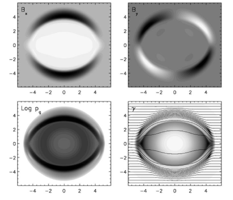
Figure 9: Gray scale levels of the $x$ component of magnetic field (top left), $y$ component of magnetic field (top right), gas pressure logarithm (bottom left) and Lorentz factor (bottom right) for the cylindrical blast wave with relatively weak magnetic field at $t=4$. Magnetic field lines are plotted on top of the Lorentz factor distribution. Following KO, we use 32 equally spaced contour levels between $0.008$ and $0.35$ (for $B_{x}$), $-0.18$ and $0.18$ (for $B_{y}$), $-4.5$ and $-1.5$ (for $\textrm{Log}\;p_{g}$), $1$ and $4.57$ (for $\gamma$).

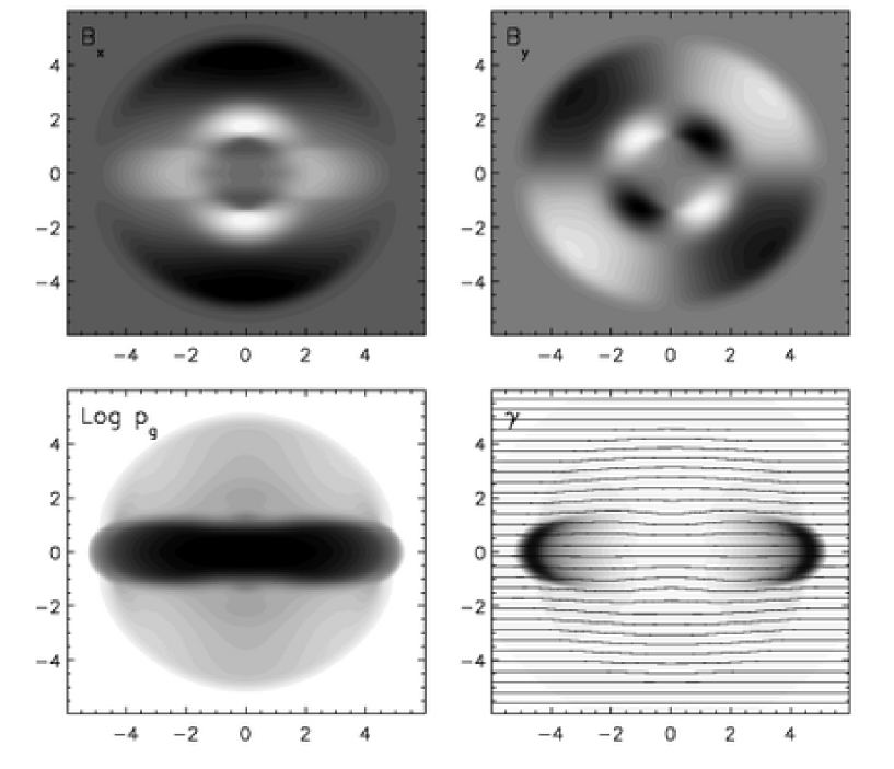
Figure 10: Cylindrical explosion for the strong magnetic field case ($B_{x}=1$). We use 32 equally space contour levels between $0.793$ and $1.116$ (for $B_{x}$), $-0.09$ and $0.09$ (for $B_{y}$), $-4.52$ and $-1.02$ (for $\textrm{Log}\;p_{g}$), $1$ and $4.23$ (for $\gamma$).

Cylindrical explosions in cartesian coordinates are particular useful in checking the robustness of the code and the algorithm response to different kinds of degeneracies. Here we follow the same setup adopted by KO, where the square $[-6,6]\times[-6,6]$ is filled with a uniform ($\rho=10^{-4}$, $p_{g}=3\cdot 10^{-5}$), initially static ($\mn@boldsymbol{v}=\mn@boldsymbol{0}$) medium, threaded by a constant magnetic field $\mn@boldsymbol{B}=(B_{x},0)$. The circular region $\sqrt{x^{2}+y^{2}}<0.08$ is initialized with constant higher density and pressure values, $\rho=0.01$ and $p_{g}=1$ decreasing linearly for $0.08\leq r\leq 1$. We adopt the ideal equation of state (15) with specific heat ratio $\Gamma=4/3$. We consider two setups, corresponding to a relatively weak magnetic field $B_{x}=0.1$ and a strong field $B_{x}=1$. Figures 9 and 10 show the magnetic field distribution, thermal pressure and Lorentz factor for the two configurations at $t=4$. Computations are carried using the van Leer limiter, eq. (65), together with the multidimensional limiting procedure described in §A.2 on $200\times 200$ uniform grid zones. The Courant number is $0.4$.

The expanding region is delimited by a fast forward shock propagating (nearly) radially at almost the speed of light. In the weak field case, a reverse shock delimits the inner region where expansion takes place radially. Magnetic field lines are squeezed in the $y$ direction building up a shell of higher magnetic pressure. In the $x$ direction the motion of the gas is not hindered by the presence of the field and it achieves a higher Lorentz factor ($\gamma_{\max}=4.39$). In the strong field case, the expansion is magnetically confined along the $x$ direction and the outer fast shock has reduced amplitude. The maximum Lorentz factor is $\gamma_{\max}=4.02$.

We point out that numerical integrations for this test were possible only by locally redefining the total energy at the end of the time step:

$$E\rightarrow E+\frac{\bar{\mn@boldsymbol{B}}_{fa}^{2}-\bar{\mn@boldsymbol{B}}_{c}^{2}}{2}\;,$$ (76)

where $\bar{\mn@boldsymbol{B}}_{c}$ is the cell-centered magnetic field obtained after the Godunov step, whereas $\bar{\mn@boldsymbol{B}}_{fa}$ is the new magnetic field obtained by averaging the face centered values given by (72). Notice that equation (76) only redefines the energy contribution of the magnetic field that is not directly coupled to the velocity, see eq. (12) and thus may be regarded as a first-order correction. In this respect, the energy correction we propose is the same usually adopted in CT schemes, see Balsara & Spicer (1999), Tóth (1997). Although this optional step results in a slight loss of energy conservation at the discretization level, it was nevertheless found to become particularly useful in problems where the magnetic pressure dominates over the thermal pressure by more than two order of magnitudes.

4.3.2 Relativistic Shock-Cloud Interaction

The interaction of a strong relativistic fast shock with a cloud is considered on the unit square $[0,1]\times[0,1]$ in 2-D cartesian coordinates $(x,y)$. This problem has been extensively used for testing classical MHD codes see (Dai & Woodward, 1994; Tóth, 1997, and references therein). Here we consider a relativistic extension adopting a somewhat different initial condition, with magnetic field orthogonal to the slab plane. The shock wave travels in the positive $x$-direction and is initially located at $x=0.6$. Upstream, for $x>0.6$, the flow is highly supersonic with pre-shock values given by $(\rho,\gamma_{x},p_{g},B_{z})_{\textrm{pre}}=(1,10,10^{-3},0.5)$, where $\gamma_{x}=(1-v_{x}^{2})^{-\frac{1}{2}}$. In this reference frame, shocked material is at rest with values given by

$$\left(\begin{array}[]{c}\rho\\ \vskip 6.0pt plus 2.0pt minus 2.0pt\cr p_{g}\\ \vskip 6.0pt plus 2.0pt minus 2.0pt\cr B_{z}\end{array}\right)_{\textrm{post}}=\left(\begin{array}[]{c}42.5942\\ \vskip 6.0pt plus 2.0pt minus 2.0pt\cr 127.9483\\ \vskip 6.0pt plus 2.0pt minus 2.0pt\cr-2.12971\\ \vskip 6.0pt plus 2.0pt minus 2.0pt\cr\end{array}\right)\;.$$ (77)

Notice that the magnetic field carries a rotational discontinuity and the compression factor of density across the shock in not limited to $7$ (we use $\Gamma=4/3$) as in the classical case, but achieves a much higher value ($\approx 43$). This feature is unique to relativistic flows.

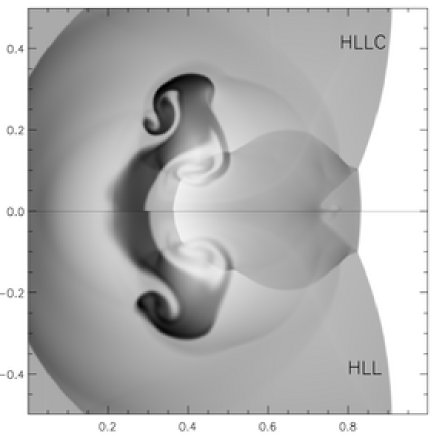
Figure 11: Density gray scale map of the interaction between a strong shock and a cloud at $t=1$. The upper and lower halves show the solutions computed with HLLC and HLL solvers, respectively, on $400\times 200$ zones, with CFL = $0.4$ and the MC limiter. Shock-flattening has been used to prevent spurious oscillations in proximity of the slow moving shock.

A circular density clump with $\rho=10$ and radius $r=0.15$ is placed ahead of the shock front, centered at $(x,y)=(0.8,0.5)$. Transverse velocities $v_{y}$ and $v_{z}$ and the $x$ and $y$ components of magnetic field are set to zero everywhere. We use $400\times 200$ computational zones, by assuming reflecting boundary at $y=0.5$ and free flow across the remaining boundaries. The MC limiter, eq. (63), is employed everywhere except in proximity of strong shocks where we revert to the minmod limiter, see §A.1. The Courant number is $0.4$.

Shortly after the impact, the cloud undergoes strong compression with the density rising by a factor of more than $20$. The collision generates a bow fast shock propagating in the shocked material and a reverse shock is transmitted into the cloud. After the transmitted shock reaches the back of the cloud, the two bent parts of the original incident shock join back together and complicated wave pattern emerges. By $t=1$ the cloud is completely wrapped by the incident shock, and the cloud expands in the form of a mushroom-shaped shell, see upper half of Fig. 11. The solution computed with the HLL solver (lower half in Fig. 11) show similar structures, although the amount of numerical viscosity is considerably higher.

Notice that, because of the assumed slab symmetry, the condition $\mn@boldsymbol{v}\cdot\mn@boldsymbol{B}=0$ is preserved in time and the solution to the Riemann problem at each interface consists of a three wave pattern: two fast waves separated by a tangential discontinuity. In this regard, our HLLC solver provides a better approximation of the full wave structure.

4.3.3 Relativistic Jet

As a final example, we consider the propagation of an axisymmetric jet in cylindrical coordinates $(r,z)$. The configuration adopted here corresponds to model C2-pol-1 in Leismann et al. (2005).

The domain $[0,12]\times[0,50]$ (in units of jet beam) is initially filled with a static uniform distributions of density, gas pressure and magnetic field, given respectively by

$$\rho_{a}=1\,,\quad p_{a}=\frac{\eta v_{b}^{2}}{\Gamma(\Gamma-1)M^{2}-\Gamma v_{b}^{2}}\,,\quad B_{z}=\sqrt{2p_{a}}.$$ (78)

The numerical value of $p_{a}$ follows from the definitions of the beam Mach number $M=v_{b}/c_{s}=6$, jet to ambient density ratio $\eta=10^{-2}$ and beam axial velocity $v_{b}=0.99$. The ideal equation of state (15) is used with $\Gamma=5/3$. The jet nozzle is located at the lower boundary $r\leq 1$, $z=0$, where boundary conditions are held constant in time, $(\rho,v_{r},v_{z},B_{r},B_{z},p_{g})=(\eta,0,v_{b},0,B_{z},p_{a})$. For $r>1$ we prescribe boundary values with antisymmetric profiles for axial velocity and radial magnetic field. Symmetric profiles are imposed on the remaining quantities. This configuration corresponds to a twin counter jet propagating in the opposite direction. Outflow boundaries are imposed on all other sides, except at $r=0$ where reflecting boundary conditions are used. We employ a uniform resolution of $20$ zones per beam radius and carry integration until $t=126$ with $CFL=0.4$.

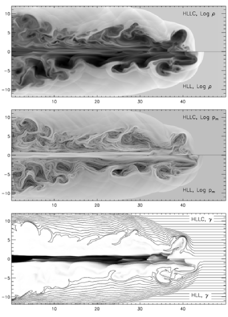
Figure 12: Gray scale images of density (top panel), magnetic pressure (middle panel) and Lorentz factor (bottom panel) for the axisymmetric jet. The upper (lower) half in each panel refers to the integration carried with the HLLC (HLL) solver. Both integrations were carried till $t=126$ with CFL = $0.8$ and the Van Leer limiter. An ideal equation of state is used with $\Gamma=5/3$. Magnetic field lines are plotted on top of the Lorentz factor gray-scale images.

The results are shown in Fig. 12, where we display density logarithm (upper panel), magnetic pressure (middle panel) and Lorentz factor distributions (lower panel). In each panel, the upper and lower halves show the solutions obtained with the HLLC and HLL solvers, respectively. As we already pointed out in the non magnetic case (Paper I), the HLLC integration features considerably less amount numerical diffusion as evident from the richness in small scale structures, notably in the density distribution. In fact, density is the physical quantity more sensitive to the introduction of the tangential wave in the Riemann solver. Comparing our results with those of (Leismann et al., 2005, see their Fig. 5) we can observe that our solution has a similar (or even larger) richness in fine structure details at half the resolution (20 ppb in our case, 40 ppb in their case).

5 Conclusions

An HLLC approximate Riemann solver has been developed for the relativistic magnetohydrodynamic equations. The new approach improves over the single state HLL solver in the ability to capture exactly isolated tangential and contact discontinuities. Several test problems in one and two dimensions demonstrate better resolution properties and a reduced amount of the numerical diffusion inherent to the averaging process of the single state HLL scheme. The solver is well-behaved for strictly two-dimensional flows, although applications to genuinely three-dimensional problems may suffer from a pathological singularity when the component of magnetic field normal to a zone interface approaches zero. This feature does not persist in the classical limit.

Multidimensional integration has been formulated in a versatile and efficient way within the framework of the corner transport upwind (CTU) method. The algorithm is stable up to Courant numbers of $1$ and preserves the divergence-free condition via constrained transport evolution of the magnetic field. The additional computational cost and the numerical implementation in an existing relativistic MHD code are minimal.

Appendix A

A.1 Shock Flattening

For strong shocks, we found that the one-dimensional prescriptions (63) or (65) can still produce spurious numerical oscillations eventually leading to the occurrence of negative pressures. A weak form of flattening is introduced by replacing eq. (63) or (65) with the minmod limiter whenever a strong shock is detected. In order for the latter condition to hold, we require that both $\nabla\cdot\mn@boldsymbol{v}<0$ and $\chi_{\min}=0$, where $\nabla\cdot\mn@boldsymbol{v}$ is computed by central differences whereas

$$\chi_{\min}=\min\left(\chi^{x}_{i+1,j},\chi^{x}_{i,j},\chi^{x}_{i-1,j},\chi^{y}_{i,j+1},\chi^{y}_{i,j},\chi^{y}_{i,j-1}\right)\,.$$ (79)

The switches $\chi^{x}$ and $\chi^{y}$ are designed as follows

$$\chi^{x}_{i,j}=\left\{\begin{array}[]{cc}1&\displaystyle\;\textrm{if}\quad\frac{p_{i+1,j}-p_{i-1,j}}{\min\left(p_{i+1,j},p_{i-1,j}\right)}\leq\epsilon\;,\\ \vskip 6.0pt plus 2.0pt minus 2.0pt\cr 0&\displaystyle\;\textrm{otherwise}\;,\end{array}\right.$$ (80)

$$\chi^{y}_{i,j}=\left\{\begin{array}[]{cc}1&\displaystyle\;\textrm{if}\quad\frac{p_{i,j+1}-p_{i,j-1}}{\min\left(p_{i,j+1},p_{i,j-1}\right)}\leq\epsilon\;,\\ \vskip 6.0pt plus 2.0pt minus 2.0pt\cr 0&\displaystyle\;\textrm{otherwise}\;,\end{array}\right.$$ (81)

where we set $\epsilon=5$ in all computations presented in this paper.

A.2 Multidimensional Limiting

Occasionally, we found that strong shocks propagating obliquely to the grid in highly magnetized media may benefit from an additional form of limiting, based on genuinely multidimensional constraints. When needed, we enforce the maximum and minimum interpolated values in each cell $(i,j)$ to lie within the bounds provided by the four neighboring zones $(i+1,j),(i-1,j),(i,j+1),(i,j-1)$. Specifically, denote with $\hat{q}^{\max}$ and $\hat{q}^{\min}$ the maximum and minimum values of $q\in\mn@boldsymbol{V}$ in these cells. Once the limited slopes $\delta_{x}q$ and $\delta_{y}q$ have been computed according to (63) or (65), we apply the correction

$$\delta_{x}q\rightarrow\tau\delta_{x}q\;,\quad\delta_{y}q\rightarrow\tau\delta_{y}q\;,\quad$$ (82)

where the multi-dimensional limiter $\tau$ is constructed as in Balsara (2004):

$$\tau=\min\left(1,\psi\min\left(\frac{\hat{q}^{\max}-q}{\delta^{\max}},\frac{q-\hat{q}^{\min}}{\delta^{\min}}\right)\right)\;,$$ (83)

with $\delta^{\max}=\max(|\delta_{x}q|,|\delta_{y}q|)$, $\delta^{\min}=\min(|\delta_{x}q|,|\delta_{y}q|)$. We set $\psi=2$ for density and magnetic field, $\psi=3/4$ for velocity and $\psi=1$ for thermal pressure.

References

- Aloy et al. (2000) Aloy, M. A., Müller, E., Ibáñez, J. M., Martí, J. M., & MacFadyen, A. 2000, ApjL, 531, L119
- Aloy et al. (2002) Aloy, M.-A., Ibáñez, J.-M., Miralles, J.-A., & Urpin, V. 2002, Astronomy and Astrophysics, 396, 693
- Anile & Pennisi (1987) Anile, M., & Pennisi, S. 1987, Ann. Inst. Henri Poincaré, 46, 127
- Anile (1989) Anile, A. M. 1989, Relativistic Fluids and Magneto-fluids (Cambridge: Cambridge University Press), 55
- Balsara & Spicer (1999) Balsara, D. S., Spicer, S. D. 1999, J. Comput. Phys, 149, 270
- Balsara (2001) Balsara, D. S. 2001, ApJS, 132, 83 (BA)
- Balsara (2004) Balsara, D. S. 2004, ApJS, 151, 149
- Brio & Wu (1988) Brio, M., & WU, C.-C. 1988, J. Comput. Phys., 75, 400
- Bruenn (1985) Bruenn, S. W. 1985, ApJS, 58, 771
- Bucciantini et al. (2005) Bucciantini, N., del Zanna, L., Amato, E., & Volpi, D. 2005, Astronomy & Astrophysics, 443, 519
- Colella (1990) Colella, P. 1990, J. Comput. Phys., 87, 171
- Courant et al. (1928) Courant, R., Friedrichs, K. O. & Lewy, H. 1928, Math. Ann., 100, 32
- Dai & Woodward (1994) Dai, W., & Woodward, P.R. 1994, ApJ, 436,776
- Davis (1988) Davis, S.F. 1988, SIAM J. Sci. Statist. Comput., 9, 445
- Del Zanna et al. (2003) Del Zanna, L., Bucciantini, N., & Londrillo, P. 2003, Astronomy & Astrophysics, 400, 397, (dZBL)
- Dimmelmeier et al. (2002) Dimmelmeier, H., Font, J. A., Müller, E. 2002, Astronomy and Astrophysics, 393, 523
- Duez et al. (2005) Duez, M. D., Liu, Y. T., Shapiro, S. L., & Stephens, B. C. 2005, Phys. Rev. D, 72, 024028
- Einfeldt et al. (1991) Einfeldt, B., Munz, C.D., Roe, P.L., and Sjögreen, B. 1991, J. Comput. Phys., 92, 273
- Elvis et al. (2002) Elvis, M., Risaliti, G., & Zamorani, G. 2002, ApJL, 565, L75
- Evans & Hawley (1988) Evans, C. R., & Hawley, J. F. 1988, apj, 332, 659
- Gammie et al. (2003) Gammie, C. F., McKinney, J. C., & Tóth, G. 2003, ApJ, 589, 444
- Gardiner & Stone (2005) Gardiner, T.A., & Stone, J.M. 2005, Journal of Computational Physics, 205, 509
- Giacomazzo & Rezzolla (2005) Giacomazzo, B., & Rezzolla, L. 2005, J. Fluid Mech., xxx
- Gurski (2004) Gurski, K.F. 2004, SIAM J. Sci. Comput, 25, 2165
- Harten et al. (1983) Harten, A., Lax, P.D., and van Leer, B. 1983, SIAM Review, 25(1):35,61
- Koldoba et al. (2002) Koldoba, A. V., Kuznetsov, O. A., & Ustyugova, G. V. 2002, mnras, 333, 932
- Komissarov (1997) Komissarov, S. S. 1997, Phys. Lett. A, 232, 435
- Komissarov (1999) Komissarov, S. S. 1999, mnras, 303, 343, (KO)
- Königl & Granot (2002) Königl, A., & Granot, J. 2002, ApJ, 574, 134
- Leismann et al. (2005) Leismann, T., Antón, L., Aloy, M. A., Müller, E., Martí, J. M., Miralles, J. A., & Ibáñez, J. M. 2005, Astronomy & Astrophysics, 436, 503
- Li (2005) Li S., 2005, J. Comput. Phys., 344-357
- Londrillo & Del Zanna (2000) Londrillo, P., & Del Zanna, L. 2000, ApJ, 530, 508
- Londrillo & Del Zanna (2004) Londrillo, P., & Del Zanna, L. 2005, Journal of Computational Physics, 195, 17
- Macchetto (1999) Macchetto, F. D. 1999, Astrophysics ans Space Science, 269, 269
- MacFadyen & Woosley (1999) MacFadyen, A. I., & Woosley, S. E. 1999, ApJ, 524, 262
- Martí & Müller (2003) Martí, J. M. & Müller, E. 2003, Living Reviews in Relativity, 6, 7
- Meier (2003) Meier, D. L. 2003, New Astronomy Review, 47, 667
- Meszaros & Rees (1994) Meszaros, P., & Rees, M. J. 1994, MNRAS, 269, L41
- McKinney & Gammie (2004) McKinney, J. C., & Gammie, C. F. 2004, ApJ, 611, 977
- McKinney (2005) McKinney, J. C. 2005, ApJL, 630, L5
- Mignone et al. (2005a) Mignone, A., Plewa, T., and Bodo, G. 2005, ApJS, 160, 199
- Mignone & Bodo (2005) Mignone, A., and Bodo, G. 2005, MNRAS, 364 (1), 126 (Paper I)
- Mignone et al. (2005) Mignone, A., Massaglia, S., and Bodo, G. 2005, Space Sci. Rev., in press
- Miyoshi & Kusano (2005) Miyoshi, T., & Kusano, K. 2005, Journal of Computational Physics, 208, 315
- Noh (1987) Noh, W.F. 1987, J. Comput. Phys., 72,78
- Romero et al. (2005) Romero, R., Marti, J. M., Pons, J. A., Ibanez, J. M., & Miralles, J. A. 2005, ArXiv Astrophysics e-prints, arXiv:astro-ph/0506527
- Rosswog et al. (2003) Rosswog, S., Ramirez-Ruiz, E., & Davies, M. B. 2003, MNRAS, 345, 1077
- Saltzman (1994) Saltzman, J. 1994, J. Comput. Phys., 115, 153
- Shapiro (2005) Shapiro, S. L. 2005, ApJ, 620, 59
- Tóth (1997) Tóth, G. 2000, J. Comput. Phys., 161, 605
- Toro (1997) Toro, E. F. 1997, Riemann Solvers and Numerical Methods for Fluid Dynamics, Springer-Verlag, Berlin
- Toro et al. (1994) Toro, E. F., Spruce, M., and Speares, W. 1994, Shock Waves, 4, 25
- van Leer (1977) van Leer, B. 1977, J. Computat. Phys., 23, 263
- van Putten (1993) van Putten, M.H.P.M. 1993, J. Comput. Phys., 105, 339
- Varnière et al. (2002) Varnière, P., Rodriguez, J., & Tagger, M. 2002, Astronomy and Astrophyiscs, 387, 497