Spatial Correlation Function of the Chandra Selected Active Galactic Nuclei

Abstract

We present the spatial correlation function analysis of non-stellar X-ray point sources in the Chandra Large Area Synoptic X-ray Survey of Lockman Hole Northwest (CLASXS). Our 9 ACIS-I fields cover a contiguous solid angle of 0.4 deg² and reach a depth of $3\times 10^{-15}$ ${\rm\thinspace erg}{\rm\thinspace cm}^{-2}{\rm\thinspace s}^{-1}\,$in the 2–8 keV band. We supplement our analysis with data from the Chandra Deep Field North (CDFN). The addition of this field allows better probe of the correlation function at small scales. A total of 233 and 252 sources with spectroscopic information are used in the study of the CLASXS and CDFN fields respectively.

We calculate both redshift-space and projected correlation functions in comoving coordinates, averaged over the redshift range of $0.1<z<3.0$, for both CLASXS and CDFN fields for a standard cosmology with $\Omega_{\Lambda}=0.73,\Omega_{M}=0.27$, and $h=0.71$ ($H_{0}=100h$ km s^-1 Mpc^-1). The correlation function for the CLASXS field over scales of 3 Mpc$<s<$ 200 Mpc can be modeled as a power-law of the form $\xi(s)=(s/s_{0})^{-\gamma}$, with $\gamma=1.6^{+0.4}_{-0.3}$ and $s_{0}=8.0^{+1.4}_{-1.5}$ Mpc. The redshift-space correlation function for CDFN on scales of 1 Mpc$<s<$ 100 Mpc is found to have a similar correlation length $s_{0}=8.55^{+0.75}_{-0.74}$ Mpc, but a shallower slope ($\gamma=1.3\pm 0.1$). The real-space correlation functions derived from the projected correlation functions, are found to be $r_{0}=8.1^{+1.2}_{-2.2}$ Mpc, and $\gamma=2.1\pm 0.5$ for the CLASXS field, and $r_{0}=5.8^{+1.0}_{-1.5}$ Mpc, $\gamma=1.38^{+0.12}_{-0.14}$ for the CDFN field. By comparing the real- and redshift-space correlation functions in the combined CLASXS and CDFN samples, we are able to estimate the redshift distortion parameter $\beta=0.4\pm 0.2$ at an effective redshift $z=0.94$. We compare the correlation functions for hard and soft spectra sources in the CLASXS field and find no significant difference between the two groups. We have also found that the correlation between X-ray luminosity and clustering amplitude is weak, which, however, is fully consistent with the expectation using the simplest relations between X-ray luminosity, blackhole mass, and dark halo mass.

We study the evolution of the AGN clustering by dividing the samples into 4 redshift bins over 0.1 Mpc$<z<$3.0 Mpc. We find a very mild evolution in the clustering amplitude, which show the same evolution trend found in optically selected quasars in the 2dF survey. We estimate the evolution of the bias, and find that the bias increases rapidly with redshift ($b(z=0.45)=0.95\pm 0.15$and $b(z=2.07)=3.03\pm 0.83$). The typical mass of the dark matter halo derived from the bias estimates show little change with redshift. The average halo mass is found to be $\log~{}(M_{halo}/M_{\sun})\sim 12.1$.

1 Introduction

Structure formation and evolution in the universe and the formation and growth of supermassive black holes (SMBHs) are two fundamental problems in astronomy which are still not fully understood. While recent progresses in the cosmic microwave background, the high redshift type Ia supernovae survey, and the large optical surveys have significantly improved our understanding of the evolution of large scale structure, there are still several gaps in the picture of structure formation. The data at redshift of $\sim 1$, where most of the cosmic star formation might have taken place, is still very limited. On scales of galaxies and cluster of galaxies, the feed back process from galaxies or AGNs could significantly alter structure formation models where gravitation is the only driving force. The clustering of active galactic nuclei (AGNs) provides unique path to the solution of these problems because (1) the AGNs are often bright compared to normal galaxies and are easily seen at large cosmological distance; (2) AGNs trace the violent growth phase of SMBHs and hence their clustering properties provide a link between the dark matter halo to the AGN activity. Large scale AGN surveys have been traditionally carried out in the optical band with dedicated telescopes. The most recent of these are the Sloan Digital Sky Survey (SDSS, Schneider et al. 2004) and the Two Degree Field Survey (2dF, Croom et al. 2005, C05 hereafter). These surveys have demonstrated that the clustering of AGNs can be used to measure cosmological parameters (Croom et al. 2004; Outram et al. 2004), and to constrain gravitational lensing (Myers et al. 2003). However, as has been found in recent Chandra and XMM-Newton deep surveys, a large fraction of X-ray detected AGNs show little or no activity in optical observations (e.g. Barger et al. 2005), most probably due to obscuration (Fabian & Iwasawa 1999) but possibly with some contribution from light dilution of the host galaxy (Moran, Filippenko, & Chornock 2002), though Barger et al. (2005) argue this is not a dominant factor. This results in a large fraction of AGNs being missed in the optical surveys. On the other hand, hard X-rays ($>2$ keV) is almost unaffected by obscuring column densities $N_{H}<10^{24}$ cm^-2, and the X-ray emission from the host galaxies is low compared to the AGNs. Thus hard X-rays are at present the best energy band to find AGNs (Mushotzky 2004). Recent optical follow-ups of Chandra deep surveys have revealed that the hard X-ray sources are mostly found around $z\sim 1$ instead of $z\sim 2$ as seen in optically selected quasar samples. The low redshift population is dominated by non-broadline objects, while broadline AGNs are found mostly at higher redshifts (Steffen et al. 2003). Given these new discoveries, it is important to know how the clustering properties of X-ray and optical selected AGN differ.

The most extensive X-ray AGN surveys so far performed used the ROSAT telescope (Mullis et al. 2004). Because the telescope is not sensitive above 2 keV, ROSAT misses a large fraction of hard X-ray sources . The relatively poor spatial resolution of ROSAT also limits the accuracy of optical identifications. Most of the ROSAT detected AGNs show broad emission lines in their optical spectra. Both the optical quasar surveys and the ROSAT surveys suggest that AGNs have correlation properties similar to the local galaxies. The results seem to be independant of the sample medium redshifts. This result is puzzling because AGNs are believed to be preferentially form in high density peaks where interactions between galaxies are more common, and interactions in turn are thought to be crucial in AGN fueling (Di Matteo, Springel, & Hernquist 2005). The mass of the dark matter halos that host AGNs are hence likely to be more massive.

The clustering results on hard X-ray AGNs are so far contradictory. Earlier studies of a small number of individual Chandra fields seem to indicate that the hard band number counts in these small fields has fluctuations larger than expected from Poisson noise (Cowie et al. 2002; Manners et al. 2003) but the result is contradicted with larger samples of Chandra fields (Kim et al. 2004). Basilakos et al. (2004) found a 4$\sigma$ clustering signal in hard X-ray sources at $f_{2-8keV}>10^{-14}$ ${\rm\thinspace erg}{\rm\thinspace cm}^{-2}{\rm\thinspace s}^{-1}\,$using angular correlation functions on a XMM detected AGN sample from a 2 deg² survey. A similar result was also found earlier in our 0.4 deg² Chandra field (see below) using the count-in-cells technique (Yang et al. 2003). Using the Limber equation Basilacos et al. (2004) argue that the hard X-ray sources are likely to be more strongly clustered than the optically selected AGNs. Gilli et al. (2003) reported the detection of large angular-redshift clustering in the Chandra Deep field South, which seems to be dominated by hard X-ray sources. Using the projected correlation function for the optically identified X-ray sources from the Chandra Deep field North (CDFN) and South (CDFS), Gilli et al. (2005) found that the average correlation amplitude in the CDFS is higher than that in the CDFN, and the latter is consistent with the correlation amplitude found in optically detected quasars.

In this paper, we report our spatial correlation function analysis of the optically identified X-ray sources in the Chandra Large Area Synoptic X-ray Survey of the ISO Lockman Hole Northwest region (CLASXS). CLASXS is so far the largest contiguous Chandra deep field with a high level of spectroscopic identifications. The size of the field is chosen to reduce the cosmic variance in the X-ray background to $\sim 10\%$ (Yang et al. 2004). For comparison, we have also analyzed the correlation functions for the CDFN field, using the published X-ray catalog by Alexander et al. (2003) and the optical catalog of Barger et al. (2003). Because the two surveys use basically the same optical instruments in the follow-up observations, and thus have the same accuracy in redshift measurements, the comparison is relatively straight forward. The LogN-LogS of the CDFN agrees well with that of CLASXS, also indicating that the CDFN is a “typical” field. The depth of the CDFN is very useful in probing the correlation function at small separations. In § 2 we summarize our observations and data analysis. In § 3 we discuss the methodology we use in the clustering analysis. The results of the correlation functions are presented in § 4. The evolution of AGN clustering is presented in § 5. In § 6 we discussion the implications of our results. Finally summarize our results in § 7. Throughout this paper, unless noted otherwise, we assume $H_{0}=71$ and a flat universe with $\Omega_{M}=0.27$ and $\Omega_{\Lambda}=0.73$.

2 Observations and data

CLASXS is a 0.4 deg² contiguous field centered at $\alpha=10^{h}34^{m}$, $\delta=57\arcdeg 40\arcmin$ (J2000) in the very low galactic absorption Lockman Hole Northwest region. It is the deepest 170$\mu$m survey field observed by ISOPHOT instrument on board ISO, and has recently been observed by the Spitzer Space telescope (Lonsdale et al. 2004). The Chandra observation consists of 9 ACIS-I pointings separated from each other by $\sim 10\arcmin$ to allow a close to uniform sky coverage. The center field has an exposure time of $\sim 70$ ks while the other eight pointings, have exposure times of $\sim 40$ ks. The exposure time were designed to give a uniform flux limit of $f_{2-8~{}keV}\approx 5\times 10^{-15}$ ${\rm\thinspace erg}{\rm\thinspace cm}^{-2}{\rm\thinspace s}^{-1}\,$, which is about a factor of 2 below the “knee” of the LogN-LogS curve. This choice of sensitivity allows a proper sampling of the X-ray background sources and also achieves a highest source finding efficiency.

The sub-arcsecond spatial resolution of Chandra observatory allows an unambiguous optical identification of the X-ray sources, particularly, for those which appear to be normal galaxies in optical band. Combined with follow-ups using the large Keck and Subaru optical telescopes, we identified and measured the redshifts in a large fraction of the X-ray detected AGNs in our survey. The details and the catalogs of the survey can be found in Yang et al. (2004) and Steffen et al. (2004). We performed spectroscopic observations for $\sim 90\%$ of the 525 detected X-ray sources. A total of 272 spectroscopic redshifts have been obtained, while the spectra of the rest of the sources have a signal-to-noise ratio too low to obtain secure redshift measurements. The redshift distribution of the identified sources are shown in Figure 1. The fraction of sources with spectroscopic redshift as a function of hard X-ray flux is shown in Figure 2.

The 2 Ms CDFN is so far the deepest Chandra field, reaching a flux limit of $f_{2-8keV}\approx 1.4\times 10^{-16}$ ${\rm\thinspace erg}{\rm\thinspace cm}^{-2}{\rm\thinspace s}^{-1}\,$(Alexander et al. 2003). This is $\sim 20$ times deeper than the CLASXS field. The areal density of sources in CDFN is also $\sim 5$ times higher. The optical observation were performed using the same telescope as CLASXS (Barger et al. 2003). We use the published catalog, which contains 306 sources with spectroscopic redshift. The redshift distribution of the CDFN sources is also shown in Figure 1. The fainter X-ray sources in the CDFN are more likely to be found at low redshift, $z<1$, compared to the CLASXS sources.

3 Methods

To quantify spatial clustering in a point process, the most commonly used technique is the two point correlation function. In short, a two point correlation function measures the excess probability of finding a pair of objects as a function of pair separation (Peebles 1980).

$$dP=n_{0}^{2}[1+\xi(r)]dV_{1}dV_{2}$$ (1)

where $n_{0}$ is the mean density and $r$ is the comoving distance between two sources.

Observations of low redshift galaxies and clusters of galaxies show that the correlation function of these objects over a wide range of scales can be described by a power-law

$$\xi(r)=(\frac{r}{r_{0}})^{-\gamma},$$ (2)

with $\gamma\sim 1.6-1.9$ (Peebles 1980; Peacock 1999). It should be noted that the correlation function is in fact a function of redshift, which we will discuss in § 5. Because of the small sample sizes of most of the AGN surveys, correlation functions over very wide redshift ranges are commonly used. This only makes sense if the clustering is almost constant in comoving coordinates. Fortunately, this is very close to the truth, as we shall see in § 5.

3.1 Redshift- and real-space Correlation functions

The nominal distance between sources calculated using the sky coordinates of the sources and their redshifts is sometimes called distance in redshift-space, we shall use $\bf{s}$ instead of $\bf{r}$ to indicate the distance calculated this way. It is apparent that the line-of-sight peculiar velocity of the sources could also contribute to the measured redshift (redshift distortion). This effect is most important at separations smaller than the correlation length. The projected correlation function, which computes the integrated correlation function along the line-of-sight and is not affected by redshift distortion, is often used to obtain the real-space correlation function (Peebles 1980). The projection, however, could make the correlation signal more difficult to measure. In small fields like the CDFN, the projected correlation function is also restricted by the field size, and could be affected by cosmic variance. We will calculate both the redshift-space and projected correlation functions in this paper. This allows us to estimate the effects of redshift distortion.

Following Davis & Peebles 1983, we define $\bf v_{1}$ and $\bf v_{2}$ to be the positions of two sources in the redshift-space, ${\bf s}\equiv{\bf v_{1}}-{\bf v_{2}}$ to be the redshift-space separation, and ${\bf l}\equiv({\bf v_{1}}+{\bf v_{2}})/2$ to be the mean distance to the pair of sources. We can then compute the correlation function $\xi(r_{p},\pi)$ on a two dimensional grid, where $\pi$ and $r_{p}$ are separations along and across the line-of-sight respectively:

$$\pi=\frac{{\bf s}\cdot{\bf l}}{{\bf|l|}},$$ (3)

$$r_{p}=\sqrt{{\bf s}\cdot{\bf s}-{\bf\pi}^{2}}.$$ (4)

The projected correlation function is defined as the line-of-sight integration of $\xi(r_{p},\pi)$:

$$w_{p}(r_{p})=\int_{-\pi_{max}}^{\pi_{max}}d\pi\ \xi(r_{p},\pi)=\int_{-\pi_{max}}^{\pi_{max}}dy\ \xi(\sqrt{r_{p}^{2}+y^{2}}),$$ (5)

where $y$ is the line-of-sight separation. It has been shown (Davis & Peebles 1983) that, when $\pi_{max}\rightarrow\infty$, $w_{p}(r_{p})$ satisfies a simple relation with the real-space correlation function. If a power-law form in Equation 2 is assumed, then

$$w_{p}(r_{p})=r_{p}\left(\frac{r_{0}}{r_{p}}\right)^{\gamma}\frac{\Gamma(\frac{1}{2})\Gamma(\frac{\gamma-1}{2})}{\Gamma(\frac{\gamma}{2})}.$$ (6)

In practice, the integration is not performed to very large separations because the major contribution to the projected signal comes from separations of a few times the correlation length $s_{0}$. Integrating to larger $\pi$ will only add noise to the results. After testing various scales, we found $\pi_{max}=20-40$ Mpc produces consistent results for our samples.

3.2 Correlation function Estimator

To obtain an unbiased estimate of the correlation function, we must correct for selection effects. Usually, these selection effects are treated using random samples generated with computer simulations. By comparing the simulated and observed pair distributions, the selection functions effectively cancel. We compute the correlation function using the minimum variance estimator

$$\xi=\frac{DD-2DR+RR}{RR}$$ (7)

where $DD$, $DR$ and $RR$ are the numbers of data-data, data-random and random-random pairs respectively, with comoving distances $s_{0}-\Delta s/2<s<s_{0}+\Delta s/2$ (L-S estimator, Landy & Szalay 1993). The random catalog is produced through simulations described below to account for the selection effects in observations. The random catalog usually contains a very large number of objects so that the Poisson noise introduced is negligible. We have checked our results using both L-S and the Davis-Peebles estimators (Davis & Peebles 1983) and found very good agreement between the two methods.

3.3 Uncertainties of correlation functions

There are two terms in the uncertainty of the correlation function: the statistical fluctuations and the cosmic variance. The statistical uncertainty of the correlation function is estimated assuming the error of the DR and RR pairs are zero, and the uncertainty of DD is Poissonian,

$$\sigma_{\xi}=\frac{(1+\xi)}{\sqrt{DD}}$$ (8)

In the case of small DD, where $\sqrt{DD}$ underestimates the error, we use the approximation formula (Gehrels 1986) to calculate the Poisson upper and lower limits. Since the DDs are in fact correlated, the use of Poisson errors could underestimate the real uncertainty. In the literature bootstrap resampling (Efron 1982) is often used to calculate the errors of the correlation function. The method is particularly useful in cases when the probability distribution function (PDF) of the variable is unknown, or in cases when the variables are derived from Poissonian distributed data using complex transformations, which results in rather complex PDFs. Mo, Jing, & Boerner (1992) showed that in the case of large DD, the bootstrap error is $\sim\sqrt{3}$ of the Poisson error. We use Poisson errors in our redshift-space correlation function estimates. On the other hand, we use bootstrap methods when estimating the uncertainties of the projected correlation function. This is because the numerical integration used in Equation 5 make it difficult to apply Poisson errors directly.

Cosmic variance is known to affect the estimation of the mean density when applied to small samples of normal galaxies from optical surveys. Such effect, however, is likely to be small on our X-ray selected AGN sample for the following reasons. The volumn of our survey is very large compared to the typical pensil-beam optical survey of normal galaxies that typically covers very narrow redshift ranges. On the other hand, the number density of AGNs is much lower than that of the normal galaxies, making it hard to trace individual structures at high enough sampling rate. The window function of the spectroscopic follow-up in our survey is also very flat over a wide redshift range (except in the redshift desert at $z\sim 1.2-2$). The combination of these factors makes it very difficult for a small number of structures been over sampled and thus producing incorrect estimation of the mean density. However, for ultra deep surveys with field size of a single Chandra field, small number of velocity spikes can indeed affect the correlation analysis, as seen in the case of the Chandra Deep Field South. Such structure, however, will affect number counts in the field at flux levels comparable to the depth of CLASXS. Based on the very good agreement among the number counts found in the CLASXS, CDFN, and other deep surveys (Yang et al. 2004), we believe the uncertainty from cosmic variance on the whole sample is likely to be small. However, the cosmic variance effect on subsamples could still be important, as seen in §5. In such cases, using statistical uncertainty alone could underestimates the true uncertainty.

3.4 The mock catalog

To account for the observational selection and edge effects, we perform extensive simulations to construct a mock catalog.

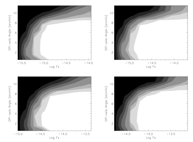
Figure 3: The probability of source detection as a function of off-axis angle and 2–8 keV fluxes. Contour levels are 0.1,0.3,0.5,0.7,0.9, 0.95,0.99. Upper(lower) panels: soft (hard) band; Left (right) panels: 70 ks exposures and 40 ks exposures.

The Chandra detection sensitivity is not uniform because of vignetting effects, quantum efficiency changes across the field and the broadening of the point spread functions. The consequence is that the sensitivity of source detection drops monotonically with off-axis angles. To quantify this we generate simulated observations of our 40 ks and 70 ks exposure in both soft and hard bands. Using wavdetect (Freeman et al. 2002) on these images we obtain an estimate of the detection probability function at different fluxes and off-axis angles (Figure 3).

With this probability, we can generate randomly distributed sources with the X-ray selection effects to the first order. We use this method instead of running detections on a large number of simulated images because the detection program runs very slowly on these images. We generate source fluxes based on the best fit LogN-LogS from Yang et al. (2004) and then “detections” are run on each of the images. The resulting catalogs from all the nine simulated images are then merged in the same way as for the real data. The resulting random source distribution and the resulting cumulative counts are shown in Figure 4.

We next consider the optical selection effects. Since our spectroscopic observation is close to complete for all sources with R$<24.5$, the sky coverage is uniform and only a very small number of sources which are very close to each other could be missed. This might reduce the power at very small scales. The redshift distribution of the sources shows a very weak dependence on the X-ray flux (Figure 5), which is due largely to the very broad luminosity function of AGNs. We can thus “scramble” the observed redshifts and assign them to the simulated sample without introducing a significant bias. The major selection effect in our optical observation is that the optical identifications are biased toward brighter sources. We select the simulated sources based on their X-ray flux using the best-fit curve in Figure 2 as a probability function. The optical selection removes a large fraction of X-ray dim sources and therefore reduces the non-uniformity in the angular distribution caused by the X-ray selection effects. The redshift of the random sources were sampled from a Gaussian smoothed ($\sigma_{z}=0.2$) redshift distribution from the observations. The purpose of the smoothing is to remove possible redshift clustering in the random sample but still preserve the effect of the selection function. We tested different smoothing scales $\Delta z=0.1-0.3$ and found the resulting correlation function effectively unchanged.

4 Results

4.1 Redshift-space correlation function

We calculate the redshift-space correlation function in the CLASXS sample for non-stellar sources with $0.1<z<3$ and 2–8 keV fluxes $>5\times 10^{-16}$${\rm\thinspace erg}{\rm\thinspace cm}^{-2}{\rm\thinspace s}^{-1}\,$, assuming constant clustering in comoving coordinates. The total number of sources in the sample is 233. The median redshift of the sample is 1.2. By comparing the number of detected pairs with separations $<20$ Mpc with that expected by simulation, we found that on scales of 20 Mpc, the significance of clustering is $6.7\sigma$.

We use the maximum likelihood method in searching for the best-fit parameters (Cash 1979; Popowski et al. 1998; Mullis et al. 2004). The method is preferable to the commonly used $\chi^{2}$ method because it is less affected by arbitrary binning. The method uses very small bins so that each bin contains only 1 or 0 DD pair. In this limit, the probability associated with each bin is close to independent. The expected number of DD pairs in each bin is calculated using the DR, RR pairs using the mock catalog. The likelihood is defined as

$${\mathcal{L}}\equiv\prod_{i}\frac{e^{-\mu_{i}}\mu_{i}^{x_{i}}}{x_{i}!}$$ (9)

where $\mu_{i}$ is the expected number of pairs in each bin and $x_{i}$ is the observed number of pairs. The likelihood ratio defined as

$$S\equiv-2\ln({\hbox{$\mathcal{L}$}}/{\hbox{$\mathcal{L}$}}_{0})$$ (10)

where $\hbox{$\mathcal{L}$}_{0}$ is the maximum likelihood. The resulting $S$ approaches the usual $\chi^{2}$ distribution. Since the maximum-likelihood does not provide a measure of the “goodness-of-fit”, we quote the $\chi^{2}$ derived from the binned correlation function (as shown in the figures) and the best-fit parameters from maximum-likelihood estimates.

We fit the correlation functions over three separation ranges. In Figure 6 we show the correlation function and the best-fit with 3 Mpc$<s<$200 Mpc. The best-fit parameters for all three separation ranges are listed in Table 1. It is noticeable that the rather large $\chi^{2}$ seems to suggest that the single power-law model may not be a proper description of the data.

For comparison, we also computed the correlation function of the X-ray sources in CDFN in the same redshift interval. We created a mock catalog 50 times larger than the observation. The positions and redshifts of the random sources are generated by randomizing the observed positions and redshifts. A large Poisson noise was added to avoid artificial clustering in the mock catalog. Such randomization is justified because the clustering signal in a small field like the CDFN mainly comes from clustering along the line-of-sight direction. The randomized sky coordinates are filtered using an image mask to take into account the edge effects. We include all the non-stellar sources in the same redshift interval as we use for CLASXS, which results in 252 sources in the sample. The best-fit parameters for CDFN field over three scale ranges are also shown in Table 1. The correlation function over 1 Mpc$<s<$100 Mpc is shown in Figure 7.

There is a good agreement of the correlation lengths obtained in the two fields. There seems to be a systematic flattening of the slope at small separations ($s\sim 10$ Mpc) in both samples. When the correlation functions are fitted at small and large separations independently, the resulting $\chi^{2}$s are systematically smaller.

4.2 Projected correlation function

The projected correlation function is computed using the methods described in § 3.1. To test the method, we first compute the projected correlation function for the CDFN and compare the results with that published in Gilli et al. (2005). We selected the same redshift interval for the CLASXS field. A two dimensional correlation function is calculated on a $5\times 10$ grid on the ($r_{p}$,$\pi$) plane. The 5 intervals along $r_{p}$ axis covers 0.16–20 Mpc. We integrate the resulting two dimensional correlation function along the line-of-sight to a $\pi_{max}=20$ Mpc. Our projected correlation function for CDFN is shown Figure 8, and it agrees perfectly with that reported in Gilli et al. (2005) for $z=0-4$, validating the techniques used in this paper.

We next compute the projected correlation function for the CLASXS field. The correlation function is calculated on scales of $r_{p}=1-30$ Mpc. The 2-D correlation function is integrated to $\pi_{max}=30$ Mpc. The result is also shown in Figure 8. The correlation functions of the CDFN and CLASXS fields agree in general at $r_{p}\sim 10$ Mpc, where both surveys have very good S/N. The slope, however, appears to be flatter in the CDFN field.

We perform a $\chi^{2}$ fit to the correlation functions using Equation 6. The best-fit parameters for the CDFN are $r_{0}=5.8^{+1.0}_{-1.5}$ Mpc, $\gamma=1.38^{+0.12}_{-0.14}$, and the reduced $\chi^{2}/dof=2.5/3$. This is in good agreement with the result from Gilli et al. (2005, $r_{0}=5.7$ Mpc, $\gamma=1.42$). The quoted errors in that paper is smaller than we obtained, but since we adopt a bootstrap error instead of Poisson error in this analysis, the difference is expected. The best-fit parameters for the CLASXS field are $r_{0}=8.1^{+1.2}_{-2.2}$ Mpc, $\gamma=2.1^{+0.5}_{-0.5}$, and the reduced $\chi^{2}/dof=1.6/4$. The correlation length appears to be higher than that of the CDFN, but agrees within the errors. The slope also seems steeper than that of the CDFN and agrees better with the slope of the redshift-space correlation function at $r_{p}>10$ Mpc. Since the CLASXS sample does not cover separations $<10$ Mpc very well, it is hard to see a slope change in this sample alone. Since the CDFN and CLASXS connect very well at separations where both surveys are sensitive, we try to model the combined data points with a single power-law. This yields $r_{0}=6.1^{+0.4}_{-1.0}$ Mpc, $\gamma_{0}=1.47^{+0.07}_{-0.10}$, and $\chi^{2}/dof=10.7/9$. The reduced $\chi^{2}$ is much worse than the two samples fitted separately, but does not reject the hypothesis of a single power-law fit. This seems to suggest that the slope of the correlation function flattens at small separations. Such a trend need to be looked more closely with future large AGN surveys with better signal-to-noise.

4.3 Redshift distortion

Redshift distortion affects the correlation function (power-spectrum) by increasing the redshift-space correlation amplitude and changing the shape of the 2-D redshift-space correlation function at small scales (such as the well known “finger-of-God” effect, e.g. Hamilton 1992). Since our data is too noisy at small separations to detect the effect, we only discuss the effect of the amplitude boosting of correlation function in redshift-space. Kaiser (1987) showed that to the first order,

$$\xi(s)=\xi(r)(1+\frac{2}{3}\beta+\frac{1}{5}\beta^{2}),$$ (11)

where $\beta\approx\Omega_{M}(z)^{0.6}/b(z)$ and $b(z)$ is bias. In principle, the redshift-space distortion can be estimated by comparing $\xi(s)$ and $\xi(r)$. To quantify the effect, we use the correlation function estimates at scales where both projected and redshift-space correlation functions are well determined. For the CDFN, we chose the correlation function estimates at 10 Mpc and find $\xi(s=10~{}Mpc)/\xi(r=10~{}Mpc)=1.75\pm 0.55$, if the best-fit of $\xi(s)$ on 1-100 Mpc is used. The choice of this scale is justified given that the slope possibly changes below and above 10 Mpc, as seen in the projected correlation function. Since the slope of the redshift- and real-space correlation function is very similar in the CDFN, the ratio is almost constant. For the CLASXS field, we chose to estimate the ratio at 20 Mpc, where the S/N is the best. We find $\xi(s=20~{}Mpc)/\xi(r=20~{}Mpc)=1.73\pm 0.42$ by using the best-fit on 1–100 Mpc for $\xi(s)$. The ratio changes slowly with the scales probed, but is within the errors. We find a general agreement between CLASXS and CDFN. To avoid the arbitrary choice of scales, and to make the best use of the data, we combine the two samples to study the redshift distortion effect on $\xi(r_{p},\pi)$. Since the projected correlation function of CDFN and and CLASXS agree in general, we are encouraged to assume that the the two samples, even with the vast difference in flux limits, generally trace the large scale structure in the same way.

In Figure 9. we show the combined $\xi(r_{p},\pi)$. The contours show no significant signature of nonlinear redshift distortion, such as the “finger-of-god”. We fit $\xi(r_{p},\pi)$ with Equation 11, assuming the best-fit parameters for the real-space correlation function from the combined sample ($r_{0}=6.1$ Mpc, $\gamma_{0}=1.47$), and ignoring the higher order redshift distortions. We generate the 2-D correlation function at each grid point. By minimizing $\chi^{2}$ by changing $\beta$, we found the best-fit $\beta=0.4\pm 0.2$, corresponding to $\xi(s)/\xi(r)\sim 1.3$, which agrees with the estimates from individual fields above. By fixing $\Omega_{M}=0.27$, we can estimate the bias factor of X-ray selected AGNs from $\beta$. The median redshift of the combined sample is 0.94, and $\Omega_{M}(z=0)=0.27$ gives $\Omega_{M}(z=0.94)=0.73$. This yields $b\approx 2.04\pm 1.02$ using the relation $\beta\approx\Omega_{M}^{0.6}/b$.

4.4 X-ray color dependence

We further test if there is any differences in clustering properties between the hard and soft spectra sources in the CLASXS sample. We use the hardness ratio, defined as $HR\equiv C_{2-8keV}/C_{0.5-2keV}$ (where $C$ is the count rate), to quantify the spectral shape of the X-ray sources. Correlation functions of soft ($HR<0.7$) and hard ($HR\geq 0.7$) sources are calculated the same way as above. The fraction of broad-line AGNs is 56.4% in the soft sample and 15.4% in hard sample. The median redshifts are 1.25 and 0.94 for soft and hard samples, respectively. We compute $\xi(s)$ for both soft and hard sources over scales of 3–200 Mpc.

Using a maximum-likelihood fit, we found $s_{0}=9.6^{+2.4}_{-3.4}$ Mpc, $\gamma=1.6^{+0.8}_{-0.6}$ for hard sources and $s_{0}=8.6^{+2.2}_{-2.0}$ Mpc, $\gamma=1.6^{+0.6}_{-0.5}$ for soft sources. We found no significant difference in clustering between the soft and hard sources. This agrees with the results of Gilli et al. (2005). It is noticeable that the soft sources have a higher median redshift than the hard sources. The interpretation of this result must include evolution effects. To avoid this complication, we restricted the redshift range to $z=0.1-1.5$. The best-fit parameters are $s_{0}=9.5^{+3.1}_{-3.7}$ Mpc ($6.2^{+2.7}_{-4.6}$ Mpc) and $\gamma=1.7^{+0.9}_{-0.6}$ ($2.5^{+1.6}_{-0.9}$) for hard (soft) sources. The difference in clustering parameters between soft and hard sources are well within the measurement error. The same analysis on CDFN yields similar results. Thus there is no significant dependence of clustering on the X-ray color.

4.5 Luminosity dependence

The cold dark matter (CDM) model of hierarchical structure formation predicts that massive (and hence luminous) galaxies are formed in rare peaks, and therefore should be more strongly clustered. This is seen in normal galaxies (e.g. Giavalisco & Dickinson 2001). Whether this relation can be extended to X-ray luminosity of AGNS is unknown. This is because the X-ray luminosity relates to the dark matter halo mass in a more complex and not well understood way. The X-ray luminosity is directly linked to the accretion process, and the process is affected by factors such as accretion rate, radiative efficiency, blackhole mass and the details of the accretion process. We have shown that at least in broadline AGNs, where the blackhole mass can be inferred from the line-width and nuclear luminosity, the Eddington ratio is close to constant over two decades of 2–8 keV luminosity (Barger et al. 2005). If this is the case for all X-ray selected AGNs, we should expect the AGN luminosity to be mainly determined by the blackhole mass, which in turn, should be closely related to the halo mass (Ferrarese 2002), even though the exact form of this relation is highly uncertain. However, optical quasar surveys such as 2dF found little evidence of a correlation between clustering amplitude and ensemble luminosity (C05), perhaps due to the small dynamical range in luminosity these surveys probe. The X-ray luminosity of sources in the CLASXS and CDFN cover a luminosity range of four orders of magnitudes, making it possible to make such a test.

The 2–8 keV rest frame luminosity $L_{x}$ is calculated from the hard band fluxes, with a K-correction made assuming a power-law spectra with photon index $\Gamma=1.8$. This yields

$$L_{x}=L_{0}(1+z)^{0.2},$$ (12)

where $L_{0}$ is the luminosity in observer’s 2-8 keV band. In Figure 10 we show $L_{x}$ vs. redshift for both CLASXS and CDFN. For a better comparison of the correlation amplitude, we adopt the averaged correlation function within $20h^{-1}$ Mpc,

$$\bar{\xi}(20)=\frac{3}{20^{3}}\int_{0}^{20}ds\xi(s)s^{2}.$$ (13)

The quantity is chosen rather than $s_{0}$ because it measures the clustering (directly linked to the rms fluctuations) regardless of the shape of the correlation function. On scales of 20 Mpc the clustering is in the linear regime of density fluctuations. The error in $\bar{\xi}(20)$ is from the single parameter $1\sigma$ confidence interval obtained by fixing the slope of the correlation function to the best-fit.

We split the CLASXS (CDFN) sample into two subsamples at $L_{x}=4.5\times 10^{43}$ ${\rm\thinspace erg}{\rm\thinspace s}^{-1}\,$($3.2\times 10^{42}$ ${\rm\thinspace erg}{\rm\thinspace s}^{-1}\,$) so that each subsample contain similar number of objects. In Table 2 we show the maximum-likelihood fits as well as $\bar{\xi}(20)$s. It should be noted that the correlation amplitude is biased in redshift space. The dominant part of this bias is characterized in Equation 11. Comparing with other observations (e.g. da Ângela et al. 2005), $\beta$ is likely a weak function of redshift in the redshift range probed by our sample, with $\beta\sim 0.4$ (§4.3), this translates to $\xi(s)/\xi(r)\sim 1.3$. We correct the $\bar{\xi}(20)$’s for this bias by dividing them by 1.3. The correlation amplitude for the more luminous sources appears to be higher than that of the less luminous sources, which qualitatively agrees with expectations that X-ray luminosity reflects the dark matter halo mass. The correlation amplitude for the more luminous subsamples are $2.3\sigma$ and $5.7\sigma$ higher than that of the less bright subsample in the CLASXS and CDFN fields, respectively. However, since the more luminous subsamples also are preferentially found at higher redshifts, the evolution in $\xi(s)$ should be taken into account.

To reduce this complication, we restrict ourselves to sources within the redshift range of 0.3–1.5, where the evolution effect is relatively small (see also § 5). In Figure 11 we show $L_{x}$ vs. $\bar{\xi}(20)$ for both CLASXS and CDFN. By reducing the redshift range, the difference in correlation amplitude between the brighter and dimmer subsample is significantly reduced, in the CDFN sample, to merely $1\sigma$. For the CLASXS field, on the other hand, the correlation amplitude for both subsamples do not show significant change. For comparison, we also plot in Figure 11 the correlation amplitude from the 2dF survey (C05). The X-ray luminosities for the QSOs in the 2dF are obtained by dividing the bolometric luminosities by 35 (Elvis et al. 1994). We perform Spearman’s $\rho$ test for correlations between $\log~{}L_{x}$ and $\bar{\xi}$. We found the correlation coefficient $\rho=0.8$ for X-ray samples, or a corresponding null probability of 20%, indicating a weak correlation between the two quantities. If the 2dF samples are added, we found $\rho=0.1$, and a null probability of 17%. This means that with the X-ray sample, we have detected a weak correlation between clustering and luminosity. We will discuss this in § 6.2.

5 Evolution of clustering

Measuring the correlation function over a wide redshift range only makes sense if the correlation function is a weak function of redshift. The best measurements of clustering of 2dF quasars at high redshift show that the correlation function indeed exhibits only mild evolution (C05). In this section, we test the evolution of clustering of X-ray selected AGNs and compare them with other survey results.

5.1 Chandra Sample

We study the evolution of clustering in both CLASXS and CDFN samples, using the redshift-space correlation function. The sources are grouped in 4 redshift intervals from 0.1 to 3. The sizes of the intervals are chosen so that the number of objects in each interval is similar in the CLASXS sample. This result in a very wide redshift bin above $z=1.5$. The correlation functions for the CLASXS, CDFN and CLASXS+CDFN fields are shown in Figures 12, 13, and 14, respectively. We group the pair separations in 10 bins in these figures to show the shape of the correlation function. In some bins there could be no DD pairs, and the correlation function is set to -1 without errors. We model the correlation functions using single power-laws and fit the data using the maximum-likelihood method. As we mentioned earlier, the method is not affected by binning. We found on 3–50 Mpc scales that a single power-law provides a good fit to the data except, for the the $z=1.5-3$ interval in the CDFN, where the sample is too sparse and have very few close separation pairs, we use a separation range of 5–200 Mpc to obtain the fit. The goodness-of-fit is quantified with $\chi^{2}$. In the case where empty bins exist, we increase the bin sizes until no bins are empty before we compute the $\chi^{2}$. The results are summarized in Table 3 and the $\bar{\xi}(20)$s as a function of redshift are shown in Figure 15. We have tested fitting the correlation functions over different scale ranges, and found no significant difference in the resulting $\bar{\xi}(20)$s.

There is only mild evolution seen in both the CLASXS and CDFN fields, in agreement with the assumption that clustering is close to constant in comoving coordinates. There are some small discrepancies between the CLASXS and the CDFN clustering strength. These discrepancies give the sense of the field-to-field uncertainty and could be resolved with future larger surveys. At the highest redshift, both samples show an increase trend of clustering, but only at the $\leq 2\sigma$ level.

5.2 Comparing with other observations

In Figure 16 we plot $\bar{\xi}(20)$ as a function of redshift for CLASXS, the combined CLASXS and CDFN, as well as results from the 2dF (C05), the ROSAT North Galactic Pole Survey (NGP, Mullis et al. 2004), and the Asiago-ESO/RASS QSO survey (AERQS, Grazian et al. 2004). We did not correct for redshift distortion for observations which uses redshift-space correlation function. This leads to overestimates of the real-space correlation amplitude.

Our correlation functions show clear agreement with the evolution trend found in C05. However, as seen in § 4.5, our measured correlation amplitude on average appears similar as that of 2dF, even though the average luminosity of latter is much higher than that of the X-ray samples. We compare the X-ray luminosities of the CLASXS and CLASXS+CDFN samples with those of the 2dF in Figure 17. The X-ray luminosities of 2dF quasars are obtained the same way as in § 4.5. The luminosity difference between the 2dF sample and X-ray samples is the largest at low redshift and decreases at higher redshift. At $z>2$, the X-ray sample and the 2dF samples have similar median luminosity. The similarity in clustering amplitude can be understood in the light of the weak correlation between AGN luminosity and clustering amplitude found in § 4.5. However, as we will see in § 6.2, a correlation between dark halo mass and the X-ray luminosity predicts a rapid increase of correlation function above $L_{x}\sim 10^{44}$ ${\rm\thinspace erg}{\rm\thinspace s}^{-1}\,$. Therefore, we should expect the optical sample being more clustered than X-ray samples at medium redshifts. Such a trend is not clearly seen in our samples.

6 Discussion

6.1 Evolution of Bias and the typical dark matter halo mass

The bias evolution of optical quasar is extensively discussed in C05. They found that the bias increases rapidly with redshift($b\sim(1+z)^{2}$). We will follow these arguments to estimate the bias evolution of the X-ray samples.

On scales of 20 Mpc, the clustering of dark matter and AGNs are both in the linear regime, i.e., $\bar{\xi}(20)<1$. This allows us to measure the bias, defined as the ratio of rms fluctuation of the luminous matter (AGNs in our case) and that of the underlying total mass, as a function of redshift by comparing the observed correlation function with the linear growth rate. In terms of correlation function, the bias can be written as

$$b^{2}\equiv\xi_{light}/\xi_{mass}.$$ (14)

The averaged correlation function of mass can be obtained using

$$\bar{\xi}_{mass}(20)=\frac{3}{(3-\gamma)J_{2}(\gamma)}(\frac{8}{20})^{\gamma}\sigma_{8}^{2}D(z)^{2}$$ (15)

where $J_{2}(\gamma)=72/[(3-\gamma)(4-\gamma)(6-\gamma)2^{\gamma}]$, $\sigma_{8}=0.84$ is the rms fluctuation of mass at $z=0$ obtained by WMAP observation (Spergel et al. 2003), and we choose the best-fit $\gamma\sim 1.5$. $D(z)$ is the linear growth factor, for which we use the approximation formula from Carroll, Press, & Turner (1992). The redshift-space distortion is taken into account to the first order through Equation 11 and the bias factor is solved numerically. The result is shown in Table 4. The estimate of $b(z=1)\sim 2.2$ in the combined sample agrees with the result from the redshift-space distortion analysis in § 4.3. In Figure 18(a) we show the bias estimates for the CDFN and CLASXS+CDFN samples. The best-fit model from C05 qualitatively agrees with the X-ray results.

The simplest model for bias evolution is that the AGNs are formed at high redshift, and evolve according to the continuity equation (Nusser & Davis 1994; Fry 1996). The model is sometimes called the conserving model or the test particle model. By normalizing the bias to $z=0$, the model can be written as

$$b(z)=1+(b_{0}-1)/D(z).$$ (16)

This model is shown in Figure 18(a) as dash-dotted line. The model produces a bias evolution which is slightly too shallow at high redshifts. The correlation function evolution based on this model is also shown in Figure 16, where it underpredicts the observed $\xi$. The model predicts a decrease of correlation function at high redshift, which is not true based on our results and that of the 2dF. This implies that the AGNs observed in the local universe are unlikely to have formed at $z\gg 2$.

One of the direct predictions of CDM structure formation scenario is that the bias is determined by the dark halo mass. Mo & White (1996) found a simple relation between the minimum mass of the dark matter halo and the bias $b$. By adopting the more general formalism by Sheth, Mo, & Tormen (2001) we can compute the “typical” dark halo mass of the sample. It should be noted that the method assumes that halos are formed through violent collapse or mergers of smaller halos and hence is best applied at large separations, where the halo-halo term dominates the correlation function. This requirement is apparently satisfied by AGNs. Following Sheth, Mo, & Tormen (2001),

$$b(M,z)=1+\frac{1}{\sqrt{a}\delta_{c}(z)}[a\nu^{2}\sqrt{a}+0.5\sqrt{a}(a\nu^{2})^{(1-c)}-\frac{(a\nu^{2})^{c}}{(a\nu^{2})^{c}+0.5(1-c)(1-c/2)}],$$ (17)

where $\nu\equiv\delta_{c}(z)/\sigma(M,z)$, a = 0.707, c = 0.6. $\delta_{c}$ is the critical overdensity. $\sigma(M,z)$ is the rms density fluctuation in the linear density field and evolves as

$$\sigma(M,z)=\sigma_{0}(M)D(z),$$ (18)

where $\sigma_{0}(M)$ can be obtained from the power spectrum of density perturbation $P(k)$ convolved with a top-hat window function $W(k)$,

$$\sigma_{0}(M)=\frac{1}{2\pi^{2}}\int{dkk^{2}P(k)|W(k)|^{2}}$$ (19)

At the scale of interest ($\sim 10$ Mpc), the power spectrum can be approximated with a power-law, $P(k)\propto k^{n}$, with $-2\lesssim n\lesssim-1$ for CDM type spectrum. Integrating Equation 19 gives

$$\sigma_{0}(M)=\sigma_{8}(\frac{M}{M_{8}})^{-(n+3)/6},$$ (20)

where $M_{8}$ is the mean mass within $8~{}h^{-1}$ Mpc.

We can then solve Equation 17 for halo mass. The resulting mass is shown in Table 4 and Figure 18(b). Consistent with what’s been found in C05 for the 2dF, the halo mass does not show any evolution trend with redshift. We found $<\log(M_{halo}/M_{\sun})>\sim 12.11\pm 0.29$, which is consistent with the 2dF estimates (C05, Grazian et al. 2004).

6.2 Linking X-ray luminosity and clustering of AGNs

We have shown that over a very wide range of luminosity, the clustering amplitude of AGNs change very little. This allows us to put useful constrains on the correlations among X-ray luminosity, blackhole mass $M_{BH}$, and the dark matter halo $M_{halo}$.

Using the equivalent width of broad emission lines as mass estimators, Barger et al. (2005) found that the Eddington ratio of broadline AGNs may be close to constant. Since the hard X-ray luminosity is an isotropic indicator of the bolometric luminosity, this implies that the blackhole mass is linearly correlated with X-ray luminosity. Barger et al. (2005) found that

$${L_{44}}=(\frac{M_{BH}}{10^{8}\hbox{$\rm\thinspace M_{\odot}$}}),$$ (21)

where $L_{44}$ is $L_{x}$ in units of $10^{44}$ ${\rm\thinspace erg}{\rm\thinspace s}^{-1}\,$. A similar result is found at low redshift using a sample of broadline AGNs with mass estimates based on reverberation mapping relations (Kaspi et al. 2000; Yang 2005). The relation, however, is only tested for broadline AGNs. Deviations from this relation is also expected at low luminosities since many low luminosity AGNs tend to have a low Eddington ratio (Ho 2005).

Blackhole mass have been shown to correlate with velocity dispersion of the spheroidal component of the host galaxies (Gebhardt et al. 2000; Ferrarese & Merritt 2000). This leads to a linear correlation between $M_{BH}$ and the mass of spherical component. This relation, however, could be different at high redshift (Akiyama 2005). How these relationships translate to the $M_{BH}-M_{halo}$ relation is also unclear and could likely be nonlinear. Ferrarese (2002) showed that $M_{BH}$ – $M_{halo}$ can be modeled with a scaling law

$$\frac{M_{BH}}{10^{8}\hbox{$\rm\thinspace M_{\odot}$}}=\kappa(\frac{M_{halo}}{10^{12}\hbox{$\rm\thinspace M_{\odot}$}})^{\lambda},$$ (22)

with $\kappa$ and $\lambda$ determined by the halo mass profile.

Combining the above and using Equation 17, we can calculate the correlation amplitude as a function of X-ray luminosity. In Figure 11 we show the model expectations compared with the observations from CLASXS, CDFN and 2dF. In calculating the bias we have assumed the nonlinear power-law index $n=3-\gamma$ in Equation 20 (Peacock 1999), with the best fit $\gamma=1.5$. The three lines represent three different halo profiles discussed in Ferrarese (2002). We found that the $L_{x}-\bar{\xi(20)}$ relation is in fact dominated by the very nonlinear relation between halo mass and correlation amplitude. The difference between different halo profiles is caused mainly by the normalization $\kappa$, or the fractional mass of blackhole mass, rather than the power-law index $\lambda$. One of the important model predictions is that the correlation between X-ray luminosity and clustering is weak below $\sim 10^{43}$ ${\rm\thinspace erg}{\rm\thinspace s}^{-1}\,$and increases rapidly above that. The lack of rapid change of correlation amplitude indicates the halo mass of AGN cannot be significantly higher than the corresponding threshold. Under the assumed cosmology and bias model, the $L_{x}-\bar{\xi(20)}$ relation based on the weak lensing derived halo mass profile (Seljak 2002) is consistent with the data, while the NFW profile (Navarro, Frenk, & White 1997) and the isothermal profile predicts a too steep correlation amplitude curve at high luminosity. However, we cannot rule out these profiles as a reasonable descriptions of the AGN host halo because of the uncertainty in the shape of the correlation function and the fractional blackhole mass in dark halos at the redshift of our sample. In Figure 11 we also mark the model dark halo mass corresponding to the Seljak (2002) mass profile. The average correlation amplitude of the combined optical and X-ray sample (dotted-line) corresponds to a halo mass of $\sim 2\times 10^{12}$ $\rm\thinspace M_{\odot}$. While the luminosity in our sample ranges over five orders of magnitudes, the range of halo mass may be much smaller. The 2dF sample has a high luminosity but has a similar or lower average correlation amplitude than that of the X-ray samples. It is possible that the optical selection technique tends to select sources with a higher Eddington ratio. The correlation amplitude of the CDFN sample at $\sim 10^{41}$ ${\rm\thinspace erg}{\rm\thinspace s}^{-1}\,$, on the other hand, is higher than the model predictions. This is expected because many AGNs with such luminosities are LINERs which are probably accreting with a low radiative efficiency.

It is now clear that the weak luminosity dependence of AGN clustering is consistent with the simplest model based on the observed $L_{x}-M_{BH}$ and $M_{BH}-M_{halo}$ relations, given the large error in the correlation functions. A large dynamical range in X-ray luminosity, as well as better measurements of correlation function, are needed to better quantify this relation. The luminosity range of the 2dF survey is too small and the optical selection method also likely is biased to high Eddington ratio sources. By increasing our current CLASXS field by a factor of a few will be helpful in better determine the luminosity dependence of AGN clustering, and to put tighter constrains on AGN hosts.

6.3 Blackhole mass and the X-ray luminosity evolution

We look again at the $M_{BH}$–$M_{halo}$ relation in the light of the mass estimates of the dark matter halos from Chandra samples. If the Ferrarese (2002) relation is independent of redshift, the nearly constant dark halo mass implies little evolution for the blackhole mass. On the other hand, strong luminosity evolution is seen since $z=1.2$ in hard X-ray selected AGNs (Barger et al. 2005). This implies a systematic decrease of the ensemble Eddington ratio with cosmic time. Barger et al. (2005) showed that the characteristic luminosity of hard X-ray selected AGNs

$$L^{\star}=L_{0}(\frac{1+z}{2})^{a},$$ (23)

where $\log(L_{0}/\hbox{${\rm\thinspace erg}{\rm\thinspace s}^{-1}\,$})=44.11$ and $a=3.2$ for $z<1.2$. Ueda et al. (2003) found a similar result with a slightly shallower slope. If the typical blackhole mass does not change with redshift, the observed luminosity evolution indicates the ensemble Eddington ratio increase by a factor of $\sim 10$ from $z=0$ to $z=1$. It is hard to understand such a change of the typical Eddington ratio with redshift. One possibility is that a large number of Compton thick AGNs at $z\sim 1$ are missed in the Chandra surveys (e.g. Worsley et al. 2005), leading to the observed strong luminosity evolution.

Alternatively, instead of $M_{BH}$–$M_{halo}$ being independent of redshift, the $M_{BH}$–$v_{c}$ could be unchanged with cosmic time, as suggested by Shields et al. (2003). This is theoretically attractive because the feedback regulated growth of blackholes implies a constant $M_{BH}$–$v_{c}$ relation. This implies that $M_{BH}$–$M_{halo}$ is in fact a function of redshift. Wyithe & Loeb (2003) proposed a model(WL model here after) showing that the blackhole mass inferred from the halo mass increases with redshift. Croom et al. (2005) show that this could lead to a close to constant Eddington ratio in the 2dF sample if the optical luminosity is used to compare with the derived $M_{BH}$. Since the correlation function is only a weak function of luminosity, as we have demonstrated in § 4.5, it is better to estimate the evolution of the Eddington ratio using the characteristic mass of the blackholes from the WL model, and the characteristic luminosity from Equation 23. In Figure 19, we show the derived ensemble Eddington ratio, assuming the dark halo mass to be constant and $\log~{}(<M_{halo}/M_{\sun}>)\sim 12.11$. (we adopt the normalization of the WL model so that it matches the prediction of $M_{BH}$ – $M_{halo}$ with a NWF type of halo profile. However, the choice of this normalization is not crucial). In the figure, we see a factor of $\sim 2-3$ change in the ensemble Eddington ratio from $z=0$ to $z=1.2$. This change, however, is smaller than the typical scatter in both the luminosity and halo mass.

6.4 Comparison with normal galaxies

We now compare our clustering results with those for normal galaxies. Using the Sloan Digital Sky Survey First Data Release, Wake et al. (2004) found that the clustering of narrow-line AGNs in the redshift range $0.055<z<0.2$, selected using emission-line flux ratios, have the same correlation amplitude as normal galaxies. Our samples are not a very good probe at these redshifts, and the best clustering analysis at a comparable redshift for normal galaxies is from DEEP2 (Coil et al. 2004). At effective redshift $z_{eff}\sim 1$, they found $r_{0}=3.19\pm 0.51$ h^-1 Mpc, and $\gamma=1.68\pm 0.07$, which translates to $\bar{\xi}(20)\sim 0.1$. The correlation amplitude from CLASXS at $z=0.9$ is $\bar{\xi}(20)\sim 0.13^{+0.12}_{-0.10}$. The clustering of AGNs in CLASXS field appear the same as the clustering of normal galaxies in DEEP2. A higher correlation is found in the CDFN. The difference shows the large uncertainty of our correlation function estimates. At higher redshifts, the best estimate for galaxy clustering is from the so called “Lyman break galaxies”, named after the technique by which they are found. Adelberger et al. (1998) found, at a typical $z\sim 3$, these galaxies tend to have similar correlation function as galaxies in the local universe, indicating they are highly biased tracers of the large scale structure. In the $\Lambda$CDM cosmology, these authors found $b=4.0\pm 0.7$. This is very similar to the bias found in the highest bin of our Chandra fields ($b=3.03\pm 0.83$), which has a median redshift of $\sim 2.0$. If we extrapolate the bias of the X-ray sources to $z=3$, the bias of X-ray sources should be $\sim 4-5$, consistent with the clustering strength of Lymann break galaxies.

7 Conclusion

In this paper we study the clustering of the X-ray selected AGNs in the 0.4 deg² Chandra contiguous survey of the Lockman Hole Northwest region. Based on our previous study, the size of the CLASXS field is large enough that the cosmic variance should not be important. We supplement our study with the published data from the CDFN. The very similar LogN-LogS of the CLASXS and CDFN suggests that the cosmic variance should not be important when the CDFN is included in the analysis. The very deep CDFN gives a better probe of the correlation function at small separations. A total of 233 and 252 non-stellar sources from CLASXS and CDFN respectively are used in this study. We use the correlation function in the redshift-space as a major tool in our clustering analysis. For the whole sample, we have also performed an analysis using the projected correlation function. This allows us to quantify the effect of redshift distortion.

We summarize our results as follows:

1. We calculated the redshift-space correlation function for sources with $0.1<z<3.0$ in both the CLASXS and CDFN fields, assuming constant clustering in comoving coordinates. We found a $6.7\sigma$ clustering signal for pairs within $s<20$ Mpc in the CLASXS field. The correlation function over scale of 3 Mpc$<s<$ 200 Mpc is found to be a power-law with $\gamma=1.6^{+0.4}_{-0.3}$ and $s_{0}=8.0^{+1.4}_{-1.5}$ Mpc. The redshift-space correlation function for CDFN on scales of 1 Mpc$<s<$ 100 Mpc is found to have similar correlation length $s_{0}=8.55^{+0.75}_{-0.74}$ Mpc, but the slope is shallower ($\gamma=1.3\pm 0.1$).

2. We study the projected correlation function of both CLASXS and CDFN. The best-fit parameters for the real-space correlation functions are found to be $r_{0}=8.1^{+1.2}_{-2.2}$ Mpc, $\gamma=2.1\pm 0.5$ for CLASXS field, and $r_{0}=5.8^{+1.0}_{-1.5}$ Mpc, $\gamma=1.38^{+0.12}_{-0.14}$ for CDFN field. Our result for the CDFN shows perfect agreement with the published results from Gilli et al. (2004). Fitting the combined data from both fields gives $r_{0}=6.1^{+0.4}_{-1.0}$ Mpc and $\gamma=1.47^{+0.07}_{-0.10}$.

3. Comparing the redshift- and real-space correlation function of the combined CLASXS and CDFN fields, we found the redshift distortion parameter $\beta=0.4\pm 0.2$ at an effective redshift $z=0.94$. Under the assumption of $\Lambda$CDM cosmology, this implies a bias parameter $b\approx 2.04\pm 1.02$ at this redshift.

4. We tested whether the clustering of the X-ray sources is dependent on the X-ray spectra in the CLASXS field. Using a hardness ratio cut at $HR=0.7$, we found no significant difference in clustering between hard and soft sources. This agrees with previous claims.

5. With the large dynamic range in X-ray luminosity, we found a weak correlation between X-ray luminosity and clustering amplitude. Using a simple model based on observations that links the AGN luminosity and halo mass, we show that the observed weak correlation is consistent with the model, except at low luminosities, where sources are likely to have lower Eddington ratio. The non-detection of a strong correlation between X-ray luminosity and clustering amplitude also suggests a narrow range of halo mass.

6. We study the evolution of the clustering using the redshift-space correlation function in 4 redshift intervals ranging from 0.1 to 3.0. We found only a mild evolution of AGN clustering in both CLASXS and CDFN samples. This qualitatively agrees with the results based on optically selected quasars from 2dF survey. The X-ray samples, however, show a similar correlation amplitude as that of the 2dF sample. This is consistent with the weak correlation between AGN luminosity and the clustering amplitude found in this work.

7. We estimate the evolution of bias by comparing the observed clustering amplitude with expectations of the linear evolution of density fluctuations. The result show that the bias increases rapidly with redshift ($b(z=0.45)\sim 0.95$ and $b(z=2.07)\sim 3.03$ in CLASXS field). This agrees with the findings from 2dF.

8. Using the bias evolution model for dark halos from Sheth, Mo & Tormen (2001), we estimated the characteristic mass of AGNs in each redshift interval. We found the mass of the dark halo changes very little with redshift. The average halo mass is found to be $\log~{}(M_{halo}/M_{\sun})\sim 12.11$.

Our results have demonstrated that deep X-ray surveys are a very useful tool in studying how AGNs trace the large scale structure. Such knowledge provides an unique window to the understanding of AGN activity, and its relation to structure formation. The higher spatial density and much better completeness compared to current optical surveys allows us to study clustering on scales only accessible to very large optical surveys such as the 2dF and the SDSS. The high spatial resolution and positional accuracy of Chandra is critical for unambiguous optical identifications. Since our results on the evolution of AGN clustering could still be affected by a small number of large scale structures, as seen in Chandra Deep Field South, larger Chandra fields are still needed to improve the measurements.

Table 1: Redshift-space Correlation Function

CLASXS Field				CDF-N Field
s range (Mpc)	$s_{0}$	$\gamma$	$\chi^{2}/dof$	s range (Mpc)	$s_{0}$	$\gamma$	$\chi^{2}/dof$
10–200	$11.4^{+1.8}_{-3.1}$	$2.4^{+1.1}_{-0.8}$	6.2/8	10–100	$11.5^{+0.8}_{-1.2}$	$2.9^{+1.4}_{-0.8}$	7.9/8
3–30	$8.15^{+1.6}_{-2.0}$	$1.2^{+0.5}_{-0.4}$	3.8 /8	1–20	$11.4^{+1.8}_{-1.4}$	$.96^{+.15}_{-.17}$	6.8/8
3–200	$8.05^{+1.4}_{-1.5}$	$1.6^{+0.4}_{-0.3}$	10.6/8	1–100	$8.55^{+.75}_{-.74}$	$1.3\pm 0.1$	15.0/8

Table 2: Luminosity dependance of Correlation Function

Field	z range	zmedian	$<L_{x}>$ (${\rm\thinspace erg}{\rm\thinspace s}^{-1}\,$)	$s_{0}$	$\gamma$	$\chi^{2}/dof$	$\bar{\xi}(20)$
CLASXS	0.1–3.0	1.5	$3.3\times 10^{44}$	$11.5^{+1.9}_{-2.1}$	$2.0^{+.5}_{-0.4}$	7.2/8	$0.50^{+.18}_{-.17}$
	0.1–3.0	.73	$1.5\times 10^{43}$	$7.35^{+1.9}_{-2.0}$	$1.9^{+1.2}_{.54}$	8.8/8	$.21^{+17}_{-.11}$
	0.3–1.5	1.1	$1.4\times 10^{44}$	$11.0\pm 2.6$	$2.3^{+1.6}_{-0.6}$	9.2/8	$0.49^{+.31}_{-.23}$
	0.3–1.5	.81	$1.6\times 10^{43}$	$5.30^{+2.9}_{-3.8}$	$1.4^{+0.8}_{-0.5}$	7.8/8	$.18^{+.15}_{-.14}$
CDF-N	0.1–3.0	.98	$7.9\times 10^{43}$	$13.2\pm 2.9$	$.81^{+0.20}_{-0.17}$	8.2/8	$.74\pm 0.13$
	0.1–3.0	.51	$8.3\times 10^{41}$	$5.6^{+1.2}_{-1.1}$	$1.26^{+0.22}_{-0.20}$	11.9/8	$.22\pm.05$
	0.3–1.5	.96	$4.0\times 10^{43}$	$8.0^{+1.5}_{-1.4}$	$1.11^{+.25}_{-.22}$	11.1/8	$.39^{+.08}_{-.07}$
	0.3–1.5	.63	$1.0\times 10^{41}$	$6.8^{+1.3}_{-1.2}$	$1.28^{+.27}_{-.21}$	8.4/8	$.28\pm.07$

Table 3: Evolution of redshift-space Correlation Function

Field	z range	$<z>$	N	$<L_{x}>$	$s_{0}$	$\gamma$	$\chi^{2}/dof$	$\bar{\xi}(20)$
CLASXS	0.1–0.7	0.44	57	$1.6\times 10^{43}$	$10.6^{+3.2}_{-3.0}$	$1.3^{+0.7}_{-0.5}$	4.1/8	$0.50^{+0.20}_{-0.17}$
	0.7–1.1	0.90	60	$6.7\times 10^{43}$	$6.2^{+2.1}_{-2.8}$	$2.3^{+6.0}_{-1.0}$	5.9/8	$0.13^{+0.12}_{-0.10}$
	1.1–1.5	1.27	49	$1.1\times 10^{44}$	$6.4^{+5.0}_{-4.6}$	$1.3^{+1.2}_{-0.7}$	1.6/3	$0.25^{+0.29}_{-0.20}$
	1.5–3.0	2.00	67	$4.9\times 10^{44}$	$13.6^{+4.2}_{-5.4}$	$1.4^{+0.6}_{-0.5}$	3.1/3	$0.68^{+0.31}_{-0.34}$
CDFN	0.1–0.7	0.46	111	$2.8\times 10^{42}$	$6.8^{+0.7}_{-0.6}$	$2.2^{+0.5}_{-0.3}$	12.5/8	$0.16^{+0.04}_{-0.03}$
	0.7–1.1	0.94	91	$2.6\times 10^{43}$	$9.4^{+1.3}_{-1.4}$	$1.2^{+0.3}_{-0.2}$	5.6/8	$0.45\pm 0.08$
	1.1–1.5	1.22	28	$3.8\times 10^{43}$	$8.8^{+2.6}_{-2.3}$	$2.1^{+1.0}_{-0.8}$	2.9/8	$0.29^{+0.21}_{-0.14}$
	1.5–3.0	2.24	22	$2.4\times 10^{44}$	$14.2^{+8.5}_{-7.9}$	$2.3^{+2.2}_{-1.4}$	1.4/7	$0.89^{+1.72}_{-0.75}$
CLASXS+CDFN	0.1–0.7	0.45	168	$7.3\times 10^{42}$	$7.9^{+0.9}_{-0.9}$	$1.9^{+0.3}_{-0.3}$	5.3/8	$0.24^{+0.06}_{-0.05}$
	0.7–1.1	0.92	151	$4.3\times 10^{43}$	$10.1^{+1.1}_{-1.0}$	$1.4^{+0.2}_{-0.2}$	5.5/8	$0.45^{+0.07}_{-0.06}$
	1.1–1.5	1.26	77	$8.2\times 10^{43}$	$8.4^{+1.8}_{-2.4}$	$2.0^{+0.8}_{-0.6}$	1.8/8	$0.27\pm 0.13$
	1.5–3.0	2.07	89	$4.3\times 10^{44}$	$12.4^{+2.7}_{-3.4}$	$1.7^{+0.5}_{-0.4}$	4.2/7	$0.57^{+0.23}_{-0.24}$

Table 4: Bias evolution and dark matter halo mass

CLASXS			CLASXS+CDFN
$<z>$	$b$	$Log_{10}(M/M_{\sun})$	$<z>$	$b$	$Log_{10}(M/M_{\sun})$
0.44	$1.44\pm 0.34$	$12.54\pm 0.30$	0.45	$0.95\pm 0.15$	$11.75\pm 0.32$
0.90	$0.80\pm 0.44$	$10.85\pm 1.07$	0.92	$1.70\pm 0.17$	$12.39\pm 0.13$
1.27	$1.39\pm 0.94$	$11.84\pm 0.69$	1.26	$1.48\pm 0.46$	$11.95\pm 0.37$
2.00	$3.26\pm 1.00$	$12.47\pm 0.28$	2.07	$3.03\pm 0.83$	$12.35\pm 0.26$

Figure 1: Redshift distribution of the optically identified X-ray sources. Solid line: the CLASXS field; dashed line: the CDFN field.

Figure 2: The optical identification fraction as a function of 2–8 keV flux. Solid line shows the best-fit.

Figure 4: The right panels shows the random sources after detections. The pixel size is 0.492″. The left panels show the cumulated counts of the simulated sources (solid line) and that of the observed sources (dashed line). Top panels: hard band; bottom panels: soft band.

Figure 5: The 2–8 keV flux vs. redshift in CLASXS sample. There is no significant correlation between X-ray flux and redshift.

Figure 6: (a). The redshift-space correlation function for CLASXS field with 3 Mpc$<s<$200 Mpc. (b). Maximum-likelihood contour for the single power-law fit. Contour levels are $\Delta S=2.3,6.17,11.8$, corresponding to $1\sigma$, $2\sigma$ and $3\sigma$ confident levels for two parameter fits.

Figure 7: The same as Figure 6 for the CDFN except that the correlation function is calculated for separations 1 Mpc$<s<$100 Mpc.

Figure 8: The projected correlation function for the CLASXS, CDFN fields and the combined sample. (a)-(c) show the best-fit parameters as well as the $\chi^{2}$ contours for the CLASXS+CDFN sample, the CLASXS sample, and the CDFN sample, respectively. Contour levels are for $1\sigma$, $2\sigma$, and $3\sigma$ confident levels; (d) The projected correlation function for CLASXS (open circles) and CDFN (black dots) fields. Lines are the best-fit shown in (a)-(c). Solid line: CLASXS+CDFN; Dotted line: CLASXS; Dashed line: CDFN

Figure 9: Two dimensional redshift-space correlation function $\xi(r_{p},\pi)$ of the combined CLASXS and CDFN sample (dashed-dotted contour). Solid line shows the best-fit model. Both the data and model correlation functions are smoothed using a $2\times 2$ boxcar to reduce the noise for visualization only.

Figure 10: The luminosity of X-ray sources vs. redshifts in the CLASXS (dots) and the CDFN (open circles) samples.

Figure 11: Luminosity dependence of clustering of AGNs. Black dots: CLASXS samples; Filled boxes: CDFN samples; Diamonds: 2dF sample (Croom et al. 2004). Lines are the models for different halo profile from Farrarese (2002). Solid line: NWF profile ($\kappa=0.1$, $\lambda=1.65$); Dashed line: weak lensing determined halo profile (Seljak, 2002; $\kappa=0.67$, $\lambda=1.82$); Dash-dotted line: isothermal model ($\kappa=0.027$, $\lambda=1.82$)

Figure 12: The Redshift-space correlation function for the CLASXS field in four redshift bins. Left panels: The correlation functions and the power-law best-fits using maximum-likelihood method. Right panels: the maximum-likelihood contours for the corresponding correlation functions on the left. Contour levels correspond to $1\sigma$, $2\sigma$ and $3\sigma$ confident levels.

Figure 13: The Redshift-space correlation function for the CDFN field in four redshift bins. (layout and contour levels are the same as in Figure 12).

Figure 14: The Redshift-space correlation function for the CLASXS+CDFN field in four redshift bins. (layout and contour levels are the same as in Figure 12).

Figure 15: The evolution of clustering as a function of redshift for the CLASXS, CDFN and the two fields combined.

Figure 16: A comparison of clustering evolution in the combined Chandra fields (big dots), CLASXS field (big filled triangle), 2dF (diamonds), ROSAT NGP (filled box) and AERQS (empty box). The solid line represent linear evolution of clustering normalized to the AERQS.

Figure 17: The median luminosities of the 2dF quasar (C05) as a function of redshift (diamonds) compared to the median luminosities of CLASXS sample (triangles) and of CLASXS+CDFN sample (big dots). The lower panel shows the ratio of 2dF median luminosities to the X-ray samples.

Figure 18: (a) bias evolution.The symbols have the same meaning as in Figure 16. The solid line is the best-fit from C05. Dash-dotted line shows the linear bias evolution model. (b). The mass of host halo of the X-ray sources corresponding to the bias in panel (a).

Figure 19: Evolution of Eddington ratio. Solid line: Using luminosity function from Barger et al. (2005). Dashed line: using luminosity function from Ueda, Akiyama, Ohta, & Miyaji (2003) at $z<1.2$.

References

- Adelberger, Steidel, Giavalisco, Dickinson, Pettini, & Kellogg (1998) Adelberger, K. L., Steidel, C. C., Giavalisco, M., Dickinson, M., Pettini, M., & Kellogg, M. 1998, ApJ, 505, 18
- Akiyama (2005) Akiyama, M. 2005, ArXiv Astrophysics e-prints
- Alexander, Bauer, Brandt, Schneider, Hornschemeier, Vignali, Barger, Broos, Cowie, Garmire, Townsley, Bautz, Chartas, & Sargent (2003) Alexander, D. M., Bauer, F. E., Brandt, W. N., Schneider, D. P., Hornschemeier, A. E., Vignali, C., Barger, A. J., Broos, P. S., et al. 2003, AJ, 126, 539
- Barger, Cowie, Capak, Alexander, Bauer, Fernandez, Brandt, Garmire, & Hornschemeier (2003) Barger, A. J., Cowie, L. L., Capak, P., Alexander, D. M., Bauer, F. E., Fernandez, E., Brandt, W. N., Garmire, G. P., et al. 2003, AJ, 126, 632
- Barger, Cowie, Mushotzky, Yang, Wang, Steffen, & Capak (2005) Barger, A. J., Cowie, L. L., Mushotzky, R. F., Yang, Y., Wang, W.-H., Steffen, A. T., & Capak, P. 2005, AJ, 129, 578
- Basilakos, Georgakakis, Plionis, & Georgantopoulos (2004) Basilakos, S., Georgakakis, A., Plionis, M., & Georgantopoulos, I. 2004, ApJ, 607, L79
- Carroll, Press, & Turner (1992) Carroll, S. M., Press, W. H., & Turner, E. L. 1992, ARA&A, 30, 499
- Cash (1979) Cash, W. 1979, ApJ, 228, 939
- Coil, Davis, Madgwick, Newman, Conselice, Cooper, Ellis, Faber, Finkbeiner, Guhathakurta, Kaiser, Koo, Phillips, Steidel, Weiner, Willmer, & Yan (2004) Coil, A. L., Davis, M., Madgwick, D. S., Newman, J. A., Conselice, C. J., Cooper, M., Ellis, R. S., Faber, S. M., et al. 2004, ApJ, 609, 525
- Cowie, Garmire, Bautz, Barger, Brandt, & Hornschemeier (2002) Cowie, L. L., Garmire, G. P., Bautz, M. W., Barger, A. J., Brandt, W. N., & Hornschemeier, A. E. 2002, ApJ, 566, L5
- Croom, Boyle, Shanks, Outram, Smith, Miller, Loaring, Kenyon, & Couch (2004) Croom, S., Boyle, B., Shanks, T., Outram, P., Smith, R., Miller, L., Loaring, N., Kenyon, S., et al. 2004, in ASP Conf. Ser. 311: AGN Physics with the Sloan Digital Sky Survey, 457–+
- Croom, Boyle, Shanks, Smith, Miller, Outram, Loaring, Hoyle, & da Ângela (2005) Croom, S. M., Boyle, B. J., Shanks, T., Smith, R. J., Miller, L., Outram, P. J., Loaring, N. S., Hoyle, F., et al. 2005, MNRAS, 356, 415
- da Ângela, Outram, Shanks, Boyle, Croom, Loaring, Miller, & Smith (2005) da Ângela, J., Outram, P. J., Shanks, T., Boyle, B. J., Croom, S. M., Loaring, N. S., Miller, L., & Smith, R. J. 2005, MNRAS, 360, 1040
- Davis & Peebles (1983) Davis, M. & Peebles, P. J. E. 1983, ApJ, 267, 465
- Di Matteo, Springel, & Hernquist (2005) Di Matteo, T., Springel, V., & Hernquist, L. 2005, Nature, 433, 604
- Efron (1982) Efron, B. 1982, The Jackknife, the Bootstrap, and Other Resampling Plans (Philadelphia: SIAM)
- Elvis, Wilkes, McDowell, Green, Bechtold, Willner, Oey, Polomski, & Cutri (1994) Elvis, M., Wilkes, B. J., McDowell, J. C., Green, R. F., Bechtold, J., Willner, S. P., Oey, M. S., Polomski, E., et al. 1994, ApJS, 95, 1
- Fabian & Iwasawa (1999) Fabian, A. C. & Iwasawa, K. 1999, MNRAS, 303, L34
- Ferrarese (2002) Ferrarese, L. 2002, ApJ, 578, 90
- Ferrarese & Merritt (2000) Ferrarese, L. & Merritt, D. 2000, ApJ, 539, L9
- Freeman, Kashyap, Rosner, & Lamb (2002) Freeman, P. E., Kashyap, V., Rosner, R., & Lamb, D. Q. 2002, ApJS, 138, 185
- Fry (1996) Fry, J. N. 1996, ApJ, 461, L65+
- Gebhardt, Bender, Bower, Dressler, Faber, Filippenko, Green, Grillmair, Ho, Kormendy, Lauer, Magorrian, Pinkney, Richstone, & Tremaine (2000) Gebhardt, K., Bender, R., Bower, G., Dressler, A., Faber, S. M., Filippenko, A. V., Green, R., Grillmair, C., et al. 2000, ApJ, 539, L13
- Gehrels (1986) Gehrels, N. 1986, ApJ, 303, 336
- Giavalisco & Dickinson (2001) Giavalisco, M. & Dickinson, M. 2001, ApJ, 550, 177
- Gilli, Cimatti, Daddi, Hasinger, Rosati, Szokoly, Tozzi, Bergeron, Borgani, Giacconi, Kewley, Mainieri, Mignoli, Nonino, Norman, Wang, Zamorani, Zheng, & Zirm (2003) Gilli, R., Cimatti, A., Daddi, E., Hasinger, G., Rosati, P., Szokoly, G., Tozzi, P., Bergeron, J., et al. 2003, ApJ, 592, 721
- Gilli, Daddi, Zamorani, Tozzi, Borgani, Bergeron, Giacconi, Hasinger, Mainieri, Norman, Rosati, Szokoly, & Zheng (2005) Gilli, R., Daddi, E., Zamorani, G., Tozzi, P., Borgani, S., Bergeron, J., Giacconi, R., Hasinger, G., et al. 2005, A&A, 430, 811
- Grazian, Negrello, Moscardini, Cristiani, Haehnelt, Matarrese, Omizzolo, & Vanzella (2004) Grazian, A., Negrello, M., Moscardini, L., Cristiani, S., Haehnelt, M. G., Matarrese, S., Omizzolo, A., & Vanzella, E. 2004, AJ, 127, 592
- Hamilton (1992) Hamilton, A. J. S. 1992, ApJ, 385, L5
- Ho (2005) Ho, L. C. 2005, ArXiv Astrophysics e-prints
- Kaiser (1987) Kaiser, N. 1987, MNRAS, 227, 1
- Kaspi, Smith, Netzer, Maoz, Jannuzi, & Giveon (2000) Kaspi, S., Smith, P. S., Netzer, H., Maoz, D., Jannuzi, B. T., & Giveon, U. 2000, ApJ, 533, 631
- Kim, Cameron, Drake, Evans, Freeman, Gaetz, Ghosh, Green, Harnden, Karovska, Kashyap, Maksym, Ratzlaff, Schlegel, Silverman, Tananbaum, Vikhlinin, Wilkes, & Grimes (2004) Kim, D.-W., Cameron, R. A., Drake, J. J., Evans, N. R., Freeman, P., Gaetz, T. J., Ghosh, H., Green, P. J., et al. 2004, ApJS, 150, 19
- Landy & Szalay (1993) Landy, S. D. & Szalay, A. S. 1993, ApJ, 412, 64
- Lonsdale, Polletta, Surace, Shupe, Fang, Xu, Smith, Siana, Rowan-Robinson, Babbedge, Oliver, Pozzi, Davoodi, Owen, Padgett, Frayer, Jarrett, Masci, O’Linger, Conrow, Farrah, Morrison, Gautier, Franceschini, Berta, Perez-Fournon, Hatziminaoglou, Afonso-Luis, Dole, Stacey, Serjeant, Pierre, Griffin, & Puetter (2004) Lonsdale, C., Polletta, M. d. C., Surace, J., Shupe, D., Fang, F., Xu, C. K., Smith, H. E., Siana, B., et al. 2004, ApJS, 154, 54
- Manners, Johnson, Almaini, Willott, Gonzalez-Solares, Lawrence, Mann, Perez-Fournon, Dunlop, McMahon, Oliver, Rowan-Robinson, & Serjeant (2003) Manners, J. C., Johnson, O., Almaini, O., Willott, C. J., Gonzalez-Solares, E., Lawrence, A., Mann, R. G., Perez-Fournon, I., et al. 2003, MNRAS, 343, 293
- Mo, Jing, & Boerner (1992) Mo, H. J., Jing, Y. P., & Boerner, G. 1992, ApJ, 392, 452
- Mo & White (1996) Mo, H. J. & White, S. D. M. 1996, MNRAS, 282, 347
- Moran, Filippenko, & Chornock (2002) Moran, E. C., Filippenko, A. V., & Chornock, R. 2002, ApJ, 579, L71
- Mullis, Henry, Gioia, Böhringer, Briel, Voges, & Huchra (2004) Mullis, C. R., Henry, J. P., Gioia, I. M., Böhringer, H., Briel, U. G., Voges, W., & Huchra, J. P. 2004, ApJ, 617, 192
- Mushotzky (2004) Mushotzky, R. 2004, How are AGN Found? (ASSL Vol. 308: Supermassive Black Holes in the Distant Universe), 53
- Myers, Outram, Shanks, Boyle, Croom, Loaring, Miller, & Smith (2003) Myers, A. D., Outram, P. J., Shanks, T., Boyle, B. J., Croom, S. M., Loaring, N. S., Miller, L., & Smith, R. J. 2003, MNRAS, 342, 467
- Navarro, Frenk, & White (1997) Navarro, J. F., Frenk, C. S., & White, S. D. M. 1997, ApJ, 490, 493
- Nusser & Davis (1994) Nusser, A. & Davis, M. 1994, ApJ, 421, L1
- Outram, Shanks, Boyle, Croom, Hoyle, Loaring, Miller, & Smith (2004) Outram, P. J., Shanks, T., Boyle, B. J., Croom, S. M., Hoyle, F., Loaring, N. S., Miller, L., & Smith, R. J. 2004, MNRAS, 348, 745
- (46) Peacock, J. A. 1999, Cosmological Physics, by John A. Peacock, Cambridge University Press, January 1999. pp. 704
- Peebles (1980) Peebles, P. J. E. 1980, The large-scale structure of the universe (Research supported by the National Science Foundation. Princeton, N.J., Princeton University Press, 1980. 435 p.)
- Popowski, Weinberg, Ryden, & Osmer (1998) Popowski, P. A., Weinberg, D. H., Ryden, B. S., & Osmer, P. S. 1998, ApJ, 498, 11
- Schneider, Fan, Hall, Jester, Richards, Stoughton, Strauss, Subbarao, vanden Berk, Anderson, Brandt, Gunn, Trump, York, & York (2004) Schneider, D., Fan, X., Hall, P., Jester, S., Richards, G., Stoughton, C., Strauss, M., Subbarao, M., et al. 2004, in ASP Conf. Ser. 311: AGN Physics with the Sloan Digital Sky Survey, 425
- Seljak (2002) Seljak, U. 2002, MNRAS, 337, 774
- Sheth, Mo, & Tormen (2001) Sheth, R. K., Mo, H. J., & Tormen, G. 2001, MNRAS, 323, 1
- Shields, Gebhardt, Salviander, Wills, Xie, Brotherton, Yuan, & Dietrich (2003) Shields, G. A., Gebhardt, K., Salviander, S., Wills, B. J., Xie, B., Brotherton, M. S., Yuan, J., & Dietrich, M. 2003, ApJ, 583, 124
- Spergel, Verde, Peiris, Komatsu, Nolta, Bennett, Halpern, Hinshaw, Jarosik, Kogut, Limon, Meyer, Page, Tucker, Weiland, Wollack, & Wright (2003) Spergel, D. N., Verde, L., Peiris, H. V., Komatsu, E., Nolta, M. R., Bennett, C. L., Halpern, M., Hinshaw, G., et al. 2003, ApJS, 148, 175
- Steffen, Barger, Capak, Cowie, Mushotzky, & Yang (2004) Steffen, A. T., Barger, A. J., Capak, P., Cowie, L. L., Mushotzky, R. F., & Yang, Y. 2004, AJ, 128, 1483
- Steffen, Barger, Cowie, Mushotzky, & Yang (2003) Steffen, A. T., Barger, A. J., Cowie, L. L., Mushotzky, R. F., & Yang, Y. 2003, ApJ, 596, L23
- Ueda, Akiyama, Ohta, & Miyaji (2003) Ueda, Y., Akiyama, M., Ohta, K., & Miyaji, T. 2003, ApJ, 598, 886
- Wake, Miller, Di Matteo, Nichol, Pope, Szalay, Gray, Schneider, & York (2004) Wake, D. A., Miller, C. J., Di Matteo, T., Nichol, R. C., Pope, A., Szalay, A. S., Gray, A., Schneider, D. P., et al. 2004, ApJ, 610, L85
- Worsley, Fabian, Bauer, Alexander, Hasinger, Mateos, Brunner, Brandt, & Schneider (2005) Worsley, M. A., Fabian, A. C., Bauer, F. E., Alexander, D. M., Hasinger, G., Mateos, S., Brunner, H., Brandt, W. N., et al. 2005, MNRAS, 357, 1281
- Wyithe & Loeb (2003) Wyithe, J. S. B. & Loeb, A. 2003, ApJ, 595, 614
- Yang (2005) Yang, Y. 2005, Ph.D. Thesis
- Yang, Mushotzky, Barger, Cowie, Sanders, & Steffen (2003) Yang, Y., Mushotzky, R. F., Barger, A. J., Cowie, L. L., Sanders, D. B., & Steffen, A. T. 2003, ApJ, 585, L85
- Yang, Mushotzky, Steffen, Barger, & Cowie (2004) Yang, Y., Mushotzky, R. F., Steffen, A. T., Barger, A. J., & Cowie, L. L. 2004, AJ, 128, 1501