Chandra  Observations of Magnetic Fields and Relativistic Beaming in Four Quasar Jets

Abstract

We discuss the physical properties of four quasar jets imaged with the Chandra X-ray Observatory in the course of a survey for X-ray emission from radio jets (Marshall et al., 2005). These objects have sufficient counts to study their spatially resolved properties, even in the 5 ks survey observations. We have acquired Australia Telescope Compact Array data with resolution matching Chandra. We have searched for optical emission with Magellan, with sub-arcsecond resolution. The radio to X-ray spectral energy distribution for most of the individual regions indicates against synchrotron radiation from a single-component electron spectrum. We therefore explore the consequences of assuming that the X-ray emission is the result of inverse Compton scattering on the cosmic microwave background. If particles and magnetic fields are near minimum energy density in the jet rest frames, then the emitting regions must be relativistically beamed, even at distances of order 500 kpc from the quasar. We estimate the magnetic field strengths, relativistic Doppler factors, and kinetic energy flux as a function of distance from the quasar core for two or three distinct regions along each jet. We develop, for the first time, estimates in the uncertainties in these parameters, recognizing that they are dominated by our assumptions in applying the standard synchrotron minimum energy conditions. The kinetic power is comparable with, or exceeds, the quasar radiative luminosity, implying that the jets are a significant factor in the energetics of the accretion process powering the central black hole. The measured radiative efficiencies of the jets are of order 10^-4.

1 INTRODUCTION

Following the remarkable discovery of an X-ray luminous, 100 kpc scale jet in PKS 0637–752 (Schwartz et al., 2000; Chartas et al., 2000), we have embarked on a survey to investigate the occurrence and properties of such systems. Initial goals were to assess the frequency of detectable X-ray fluxes from radio-bright jets, to locate good targets for detailed imaging and spectral followup studies, and where possible to test models of the X-ray emission by measuring the broad-band, spatially resolved, spectral energy distributions (SED) of jets from the radio through the optical to the X-ray band (Marshall et al., 2005; Schwartz et al., 2003a, b). With an X-ray detection of 12 jets out of the first set of 20 observed, (Marshall et al., 2005), the survey has been successful in meeting these objectives. For four of these jets we have 40 to 130 total X-ray counts in our 5 ks observations. This suffices to construct broad-band spectral energy distributions, from which we can estimate magnetic fields, particle densities, Doppler beaming factors and kinetic fluxes for independent, spatially distinct emitting regions, using the models of synchrotron radiation and inverse Compton (IC) scattering on the cosmic microwave background (CMB), which we adopt below (Schwartz et al., 2003a, b). Deeper Chandra  as well as HST observations have been approved for all these sources (Perlman et al. (2004), and in preparation).

In parallel work, Sambruna et al. (2002, 2004) have undertaken a survey of 17 jetted radio quasars with Chandra and HST, with 10 exhibiting at least one knot in the Chandra images. We will compare our results with theirs in Section 4.

Our survey is described in Marshall et al. (2005) (hereafter Paper I). We selected objects from two parent samples for which radio maps had been obtained with $\sim$ 1″ – 2″ resolution at 1-10 GHz: a VLA sample (Dec $\geq$ 0°) of flat spectrum quasars with core flux densities $S_{5\rm{GHz}}\geq 1$ Jy (Murphy, Browne, & Perley, 1993) and an ATCA survey of flat spectrum Parkes quasars (Dec $<$ -20°) (Lovell, 1997), with core flux densities $S_{2.7\rm{GHz}}\geq 0.34$ Jy. Selection was then made for objects with radio jets which extend beyond 2″ from the core. The survey is comprised of sources for which we either anticipated extended structures with significant X-ray fluxes, based on scaling the extended 5 GHz flux using the X-ray to radio flux ratio of PKS 0637–752, (subsample “A”), or else selected by the morphological criteria of a one-sided linear jet (subsample “B”). PKS 0920-397 and PKS 1202-262 meet the “A” criterion, and PKS 0208-512, PKS 1030-357, and PKS 1202-262 meet the “B” criterion (Paper I). The definition of our parent samples by flat radio core spectra tends to select powerful sources with one-sided relativistic pc scale jets beamed toward our line of sight. The 5 or 2.7 GHz selection frequency emphasizes the jet rather than lobe emission.

Section 2 presents the X-ray data and defines distinct spatial regions for further analysis. Section 3 gives the broad band spectral energy distribution, and Section 4 the physical properties deduced by assuming that IC/CMB produces the X-ray emission. Section 5 discusses implications of the IC/CMB mechanism, and mentions alternate emission mechanisms. In Appendix A we estimate the systematic uncertainties in the magnetic fields and Doppler factors which we derive, and in Appendix B we present the basis for our calculation of the flux of kinetic energy carried by the jets.

2 OBSERVATIONS OF THE JETS

We observed the four quasars listed in Table 1 for about 5 ks, using ACIS-S. Data for the jets as a whole and X-ray results for the quasar cores appear in Marshall et al. (2005). We generally used the 1/4 sub-array mode to minimize pileup of the quasar core, but used the 1/8 subarray for PKS 0208-512 due to its greater flux. We requested roll angles such that the radio jet projected at least 30° away from the readout streak. Paper I (figure 1a, 1g, 1h, 1k), shows the overlay of the 8.64 ATCA GHz radio contours on the X-ray images. Figure 1 shows the X-ray images of the four jets, and defines the regions used for the joint X-ray/radio spatial analysis. The jet regions were manually placed on the X-ray images, and therefore involve a certain amount of subjectivity. The regions are labeled R with numbers increasing away from the quasar. They are intended primarily to be regions larger than the instrumental resolution, and distinct from the quasar core, so we could derive independent model parameters characteristic of distinct volumes within each jet.

Figure 1: ACIS-S X-ray counts, 0.5 to 7 keV, binned into 0$\farcs$492 pixels. The regions marked R1, R2, R3 are used for the SED plots and the analysis of spatially resolved parameters. The circles centered on the quasars have a 1$\farcs$23 radius, and enclose approximately 95% of the flux. The faintest color is one count per pixel. See text for definition of the marked regions. The straight lines give projected distances in the plane of the sky, at the redshift of each object. All images are in celestial coordinates with N up and E left, and cover 21″$\times$ 15″.

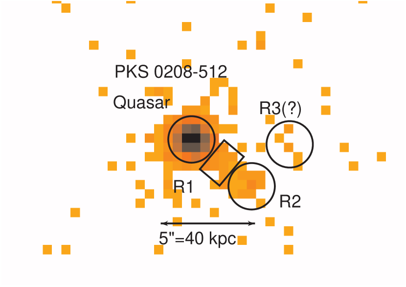
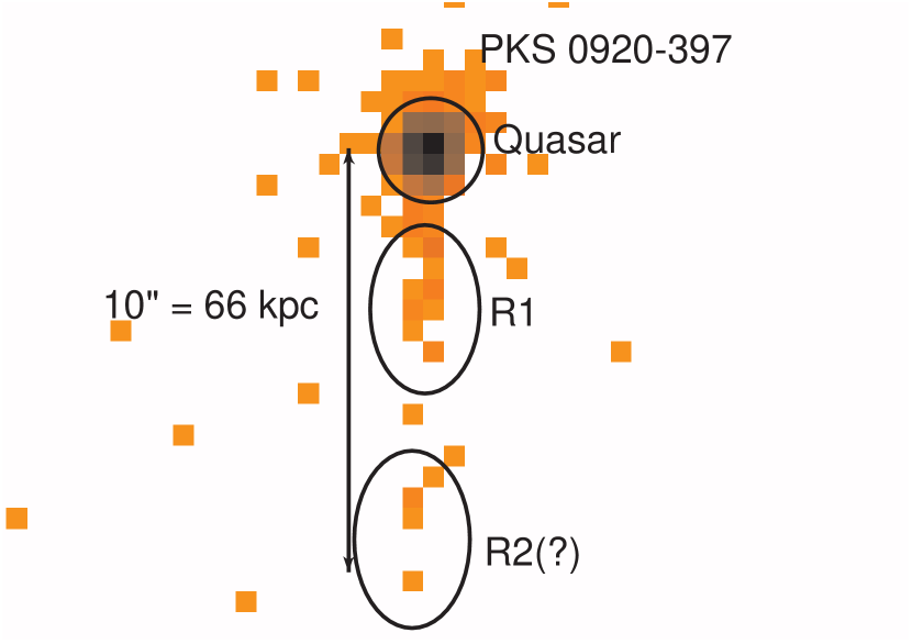
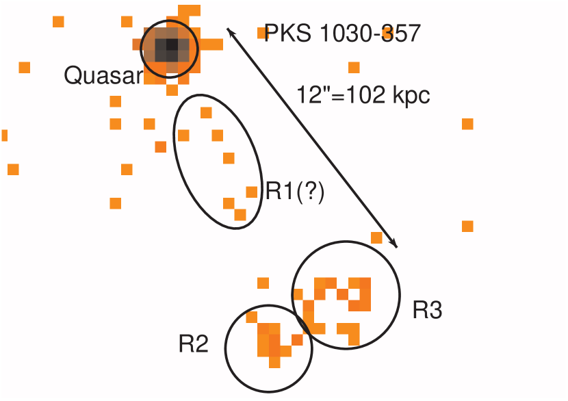
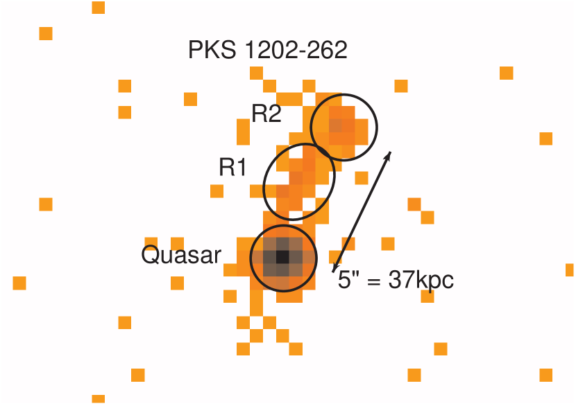
The definitions of the spatial regions included a minimum of 5 X-ray photons. Background counts are expected to be less than 0.1 in any region, and are ignored. Uncertainties are dominated by the X-ray statistics and model assumptions, as we shall discuss in Appendix A, therefore we do not believe the exact region definitions affect any of the present conclusions. However, we do note with a question mark in Table 1 three regions for which there are less than 10 X-ray counts. The reality of detection and spatial location of these, and therefore their association with the radio jet, must be regarded as less certain.

Table 1 gives the observed X-ray and radio data for each region. To derive the 1-keV X-ray flux density, $f_{1\,keV}$, and 2–10 keV rest frame luminosity, L_x, we assume a power-law energy index of $\alpha$=0.7, where $f_{\nu}\propto\nu^{-\alpha}$. Our model that the radio and X-rays arise from the same simple power-law population of electrons implies that this is also the index of the radio emission. For 3 of the quasars in Table 1 this is consistent with the spectral index from 4.8 to 8.6 GHz, $\alpha_{4.8}^{8.6}$, as tabulated in column 9, within errors whose effect will be discussed in Appendix A. For PKS 0208-512 the indices deviate markedly from $\alpha$=0.7; nevertheless we perform the formal calculation using the same index for comparison with the other objects. For this source, we have contamination of the R1 4.8 GHz flux density by the core, and the R2 and R3 regions may be a hotspot and extended lobe, and so require different modeling. Our deeper Chandra and 20 GHz ATCA observations of this source will address these issues in the future.

The X-ray properties reported here differ slightly from those in Paper I, because that paper considered the complete jet region, while in this work we omit some counts outside the regions marked in Figure 1. The angular sizes of the radio and X-ray regions are calculated by subtracting in quadrature the 1$\farcs$2 FWHM of the 8.6 GHz images given in Paper I from the dimensions of each region. The regions are all resolved in the 8.6 GHz beam. We consider the regions as cylinders of angular length, $\theta_{l}$, and diameter $\theta_{d}$. We use a flat, accelerating cosmology, with H₀=71 km s^-1 Mpc^-1, $\Omega_{\rm m}=0.27$, and $\Omega_{\Lambda}=0.73$.

Table 1: Observations of Quasars, and X-Ray Jet Regions

PKS Name		Exposure	X-ray	f${}_{\rm{1\,keV}}$		f${}_{\rm{4.8\,GHz}}$	f${}_{\rm{8.6\,GHz}}$	$\alpha_{4.8}^{8.6}$	$\theta_{l}$	$\theta_{d}$
(region)	z	Time [ks]	Counts	[nJy]	Lx	[mJy]	[mJy]		[arcsec]	[arcsec]
0208-512	0.999	5.014	1556	319	8.9	3270	3020	0.1	$\cdots$	$\cdots$
(R1)			16	3.3	0.091	$\cdots$	12.8	$\cdots$	$<$0.50	2.14
(R2)			23	4.7	0.131	25.3	25.5	-0.0	1.93	1.01
(R3)?			7	1.4	0.040	16.6	7.7	1.3	1.05	1.99
0920-397	0.591	4.466	520	120	0.973	1740	1570	0.2	$\cdots$	$\cdots$
(R1)			19	4.4	0.036	$\cdots$	38.4	$\cdots$	3.68	0.62
(R2)?			5	1.2	0.009	105	66.8	0.8	1.56	1.30
1030-357	1.455	5.029	395	80.8	5.39	241	173	0.6	$\cdots$	$\cdots$
(R1)?			7	1.4	0.095	28	22.4	0.4	5.88	0.47
(R2)			17	3.5	0.232	22.2	14.5	0.7	1.25	0.42
(R3)			28	5.7	0.382	53.8	36.2	0.7	2.89	0.84
1202-262	0.789	5.074	754	153	2.44	464	482	-0.1	$\cdots$	$\cdots$
(R1)			57	11.6	0.185	32.1	22.7	0.6	2.91	0.35
(R2)			50	10.1	0.162	45.7	31.2	0.7	0.91	0.75

Note. — Region designations followed with a question mark contain fewer than 10 X-ray counts, so their physical association with the radio emission is not certain.

3 SPECTRAL DISTRIBUTIONS

Figure 2 plots the spectral energy distributions for each of the regions shown in Figure 1. We have obtained Magellan optical observations of the four quasars (Gelbord et al. (2003, 2004), Gelbord and Marshall, in preparation 2005). In general no statistically significant optical emission is detected. An exception is R2 of PKS 0920-397; however, there are other faint optical objects in the field and we cannot rule out a chance superposition at present. We therefore treat all optical data as upper limits.

Figure 2: Spectral energy distributions for the distinct regions of each jet. The downward arrows are our upper limit to the optical flux from any region. We use a circle, square, and triangle, respectively, to indicate regions progressively further from the quasar.

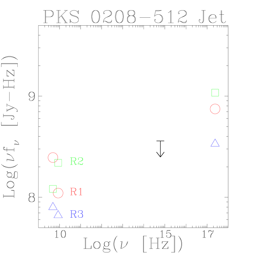
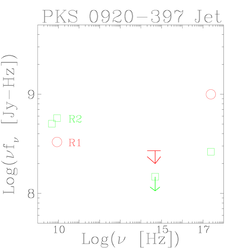
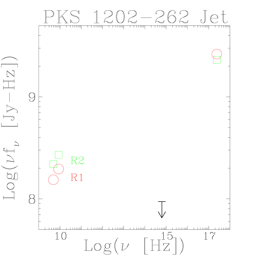
For PKS 0920-397, PKS 1030-357 and PKS 1202-262 our upper limit g^′ magnitudes do not allow the X-rays to be a simple power-law extrapolation of the radio synchrotron emission. For PKS 0208-512 our limit of 25th magnitude prevents such an extrapolation for R2. The 4.8 to 8.6 GHz radio index for PKS 0208-512 R1 and R3 also argues against extrapolation of the synchrotron emission to the X-ray region.

We will present the interpretation of all four objects in the context of inverse Compton emission from the cosmic microwave background. This has been argued to be the most plausible mechanism for the X-ray jet in many powerful radio-loud quasars (Tavecchio et al., 2000; Celotti et al., 2001; Marshall et al., 2001; Sambruna et al., 2001, 2002, 2004; Harris & Krawczynski, 2002; Siemiginowska et al., 2002, 2003a, 2003b). We discuss the consequences and limitations of this assumption, and mention alternate emission mechanisms in section 5.

4 PHYSICAL PARAMETERS

We assume that the X-ray emission from each region arises from inverse Compton scattering by the same power-law population of electrons, $n(\gamma)=n_{0}\,\gamma^{-m}$ electrons cm^-3 per unit $\gamma$, emitting the radio-synchrotron radiation from that region. The ratio of synchrotron to Compton power is just the ratio of energy density of the magnetic field to the energy density of the target photons, assuming the latter are isotropic in the jet rest frame (Felten & Morrison, 1966). In applying that formalism to the powerful X-ray jets, one typically cannot find a credible source of target photons if one also assumes that the magnetic field and relativistic electrons are nearly in energy equipartition, and are not in relativistic motion (e.g., Schwartz et al., 2000). Tavecchio et al. (2000) and Celotti et al. (2001) resolved this dilemma by exploiting the enhanced apparent CMB density for electrons moving with bulk relativistic velocity, $\beta c\approx c$, with respect to the isotropic CMB frame (Dermer & Schlickeiser, 1994). In the frame of a jet moving with bulk Lorentz factor $\Gamma$, the CMB energy density will exceed the magnetic field energy density at redshifts

$$z\geq\max{[(0.556\sqrt{B_{\mu G}/\Gamma}-1),0]},$$ (1)

(Schwartz, 2002), where B_μG is the magnetic field in micro-Gauss (1$\mu$G=0.1nT), and $\Gamma$=(1-$\beta^{2}$)^-1/2. Under such conditions the IC/CMB may become the dominant energy loss mechanism for the relativistic electrons. The energy density due to the radiation field of a quasar emitting an isotropic, bolometric luminosity 10${}^{44}\,{\rm L}_{44}$ ergs s^-1, falls below the CMB energy density at a distance 4.7 $\sqrt{(}{\rm L}_{44}/(1+{\rm z})^{2}$ kpc from the quasar. For PKS 0208-512 this distance is 34 kpc, so the quasar radiation field may play a role, especially in producing $\gamma$-ray emission. We will consider this in more detail in connection with our deeper Chandra and HST observations (Perlman et al., in preparation). For the other three objects, the quasar field drops below the CMB energy density 7 to 14 kpc from the quasar, which is much smaller than the deprojected distances we derive for the X-ray emitting regions.

From Felten & Morrison (1966), following their approximations that the flux density at any frequency is produced by a $\delta$-function at a characteristic mean electron $\gamma$, and that magnetic fields, particles, and target photons are isotropic in the emitting region, the ratio of synchrotron to IC/CMB emission, extrapolated to some common frequency, will be

$$(S_{\rm synch}/S_{\rm IC})\approx\frac{(2\times 10^{4}T)^{(3-m)/2}\,B_{\mu G}^{(1+m)/2}}{8\pi\,\rho}$$ (2)

where $\rho=\Gamma^{2}(1+z)^{4}\rho_{0}$ is the mean energy density of the CMB at redshift z in a frame moving with Lorentz factor $\Gamma$, $\rho_{0}$ = 4.19 $\times 10^{-13}$ ergs cm^-3 is the local CMB energy density, and the apparent temperature of the CMB in the jet frame is $T=(1+z)\Gamma T_{0}$, where the local CMB temperature is $T_{0}$=2.728°K (Fixsen et al., 1996). There are two independent parameters among the direction to our line of sight, $\theta$, the bulk Lorentz factor, $\Gamma$, and the effective Doppler factor $\delta$=$[\Gamma(1-\beta\cos(\theta))]^{-1}$. Since the asymptotic value of $\delta$ is 2$\Gamma$ for large $\Gamma$ when the jet is beamed exactly in our direction, i.e., $\cos(\theta)$=1, we make the common assumption $\Gamma=\delta$, in the absence of any information on $\theta$. We assume the spectral index $\alpha$=(m-1)/2=0.7, and use the known CMB parameters (Fixsen et al., 1996). We know that the CMB photons are highly anisotropic in the jet frame, but the photons we observe will be forward scattered by electrons moving near to the line of sight, so we approximate that they see the mean energy density. With these conditions, equation 2 gives an estimate of the magnetic field:

$${\rm B_{\mu G}}\approx 4.23\times 10^{-11}\delta(1+z)^{2.18}(S_{\rm synch}/S_{\rm IC})^{0.588},$$ (3)

where $S_{\rm IC}$ is the inferred X-ray flux density at 1 keV for the assumed spectral index $\alpha$=0.7, and $S_{\rm synch}$ is the measured radio flux density at 8.6 GHz. Appendix A discusses the sensitivity of our results to the spectral index. As noted above, the regions of PKS 0208-512 are not consistent with such a spectral index in the range 4.8 to 8.6 GHz.

Without considering relativistic beaming, we can apply the minimum energy conditions to estimate the magnetic field (Moffet, 1975):

$$B_{1}\approx 328.8(\frac{(1+k_{1})\,L_{\rm synch}\,}{\phi V})^{2/7}\,\,\rm{Gauss}$$ (4)

This formula assumes a uniform magnetic field, and isotropic particle distribution. (Other approaches to the minimum energy formulation will result in a small dependence of the exponent on $\alpha$; e.g., Worrall & Birkinshaw, 2005). We assume unit filling factor, $\phi$=1, and a ratio of proton to electron energy density, k₁=1. We take the lower and upper limits of the observed radio spectrum to be $\nu_{1}$=10⁶ Hz and $\nu_{2}$=10¹² Hz, in order to integrate over $\nu$ to get the total synchrotron luminosity, $L_{\rm synch}$. We consider the emitting volumes, $V$, to be cylinders with the measured angular lengths $\theta_{l}$ and diameters $\theta_{d}$. Appendix A illustrates our sensitivity to these assumptions. In the jet frame we have $B=B_{1}/\delta$ (Tavecchio et al., 2000; Harris & Krawczynski, 2002; Dermer & Atoyan, 2004), so that we have

$$B\delta\approx 400.8(L_{synch}/V)^{2/7}.$$ (5)

Figure 3: The Tavecchio et al. (2000) style diagrams for the regions defined in Figure 1. The intersections of equations 3 (lines increasing with $B$) and 5 (lines decreasing with $B$) give solutions for the Doppler factor $\delta$ and the magnetic field in the jet rest frame. The regions in order of increasing distance from the quasar are shown as dotted (“R1”), dashed (“R2”), and solid (“R3”).

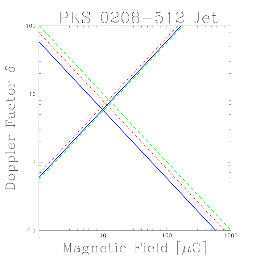
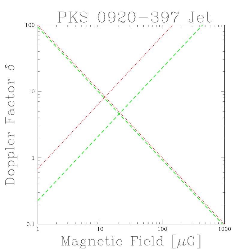
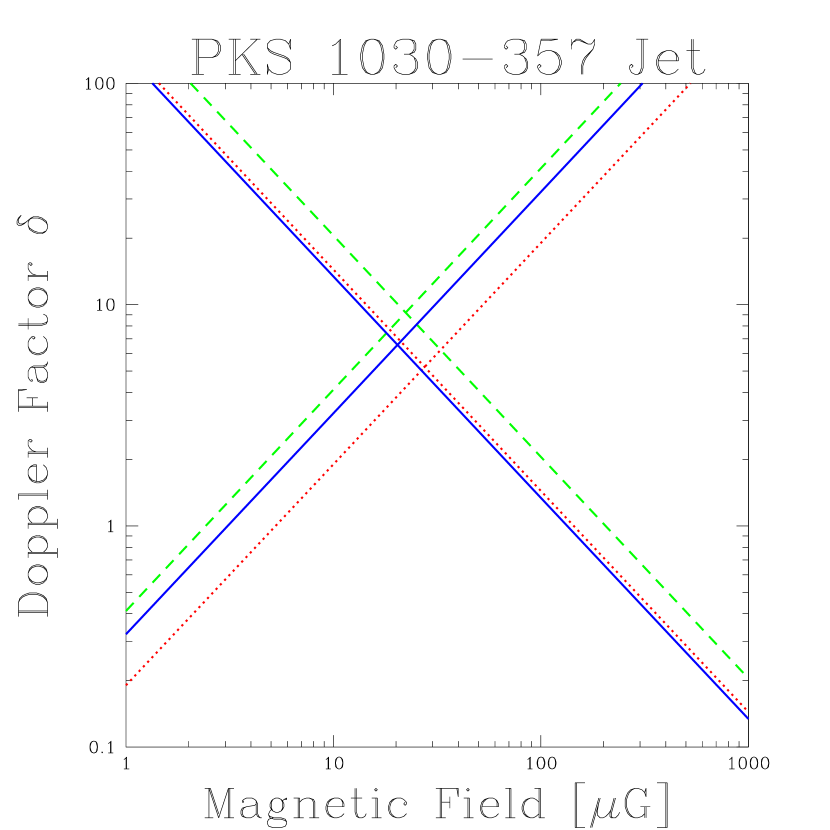
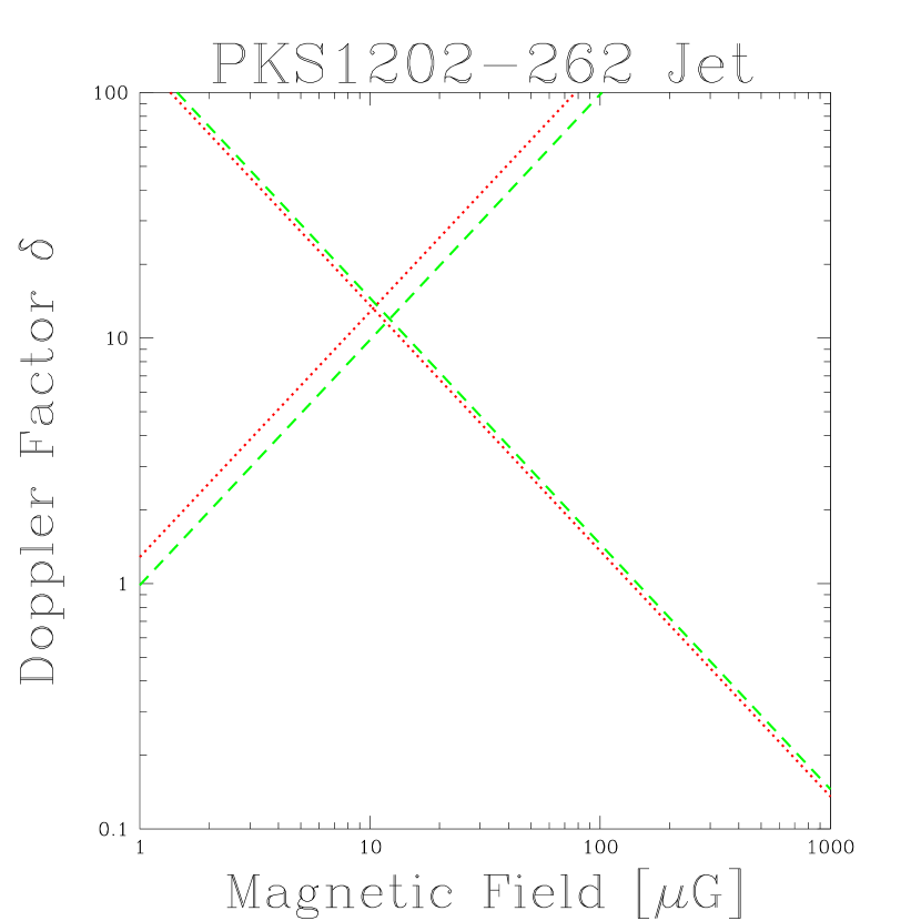
In Figure 3 we plot equations 3 and 5. The intersection of these curves for each feature in the four jets gives a solution for the unknowns $B$ and $\delta$. These values are tabulated in columns 3 and 4 of Table 2. We find magnetic fields of order 10 to 25 $\mu$G and Doppler factors in the range 5 to 15 for the various regions in the jets. In Appendix A we quantify the uncertainties on those numbers. Compared to the analysis in Paper I, which considered the entire length of the jet and which assumed $\Gamma=10$, we here use smaller volumes which naturally lead to larger values of the magnetic field B₁ and smaller angles of the jet from our line of sight.

Sambruna et al. (2004) have carried out a joint Chandra and HST survey, and report the analysis of ten knots which have been detected in both the optical and X-ray bands from six of their sources. They interpret nine of these in terms of the IC/CMB model, and derive magnetic fields in the range 3 to 12 $\mu$G, and Doppler factors in the range 6 to 14. The values derived here are therefore quite similar, despite some differences in the model assumptions; e.g., the assumed shapes of the emitting region and values of $\gamma_{min}$. As noted by Tavecchio et al. (2004), the values of the Doppler factor are expected to be relatively robust since other derived quantities depend on powers of $\delta$.

From the magnetic field strength and our arbitrary assumption of a low-frequency cutoff at an observed $\nu$ = 10⁶ Hz, we can calculate the low energy electron spectrum cutoff $\gamma_{min}$ which roughly corresponds to that frequency: $\gamma_{min}=\sqrt{(}(1+z)/(4.2\delta B))$. With that $\gamma_{min}$ we can calculate the total number density, n_e, of relativistic electrons by equating the particle energy density with that of the magnetic field, which is approximately the minimum energy condition:
$(1+k_{1})\int_{\gamma_{min}}^{\gamma_{max}}n_{0}m_{e}c^{2}\gamma^{1-m}d\gamma\approx B^{2}/(8\pi)$. Columns 5 and 6 give $\gamma_{min}$ and $n_{e}$, respectively.

For a fixed Doppler factor $\delta$, the maximum angle by which the jet can deviate from our line of sight is $\arccos[\sqrt{(}\delta^{2}-1)/\delta]$, which is also the angle for which $\delta$=$\Gamma$ as we have assumed. From this maximum angle, given in column 7 and the measured angular projection of the jet on the sky, we can compute the minimum intrinsic length of each jet region, as given in column 8 of Table 2.

Table 2: Properties of the X-Ray Jets

PKS Name	Jet	B	$\delta$	$\gamma_{min}$	ne	$\theta_{max}$	Minimum	Kinetic	Radiative
(region)	Frac	[$\mu$G]			10-8 cm-3	[deg]	Length	Flux	Efficiency
0208-512	$\cdots$	$\cdots$	$\cdots$	$\cdots$	$\cdots$	$\cdots$	$\cdots$	$\cdots$	$\cdots$
(R1)	0.010	10.9	7.3	77	1.1	7.8	156	9.5	0.3
(R2)	0.015	13.5	7.5	69	1.8	7.7	262	3.6	1.2
(R3)?	0.004	10.1	5.7	91	0.78	10.1	246	3.8	0.5
0920-397	$\cdots$	$\cdots$	$\cdots$	$\cdots$	$\cdots$	$\cdots$	$\cdots$	$\cdots$	$\cdots$
(R1)	0.037	12.1	8.3	61	1.7	6.9	322	1.0	1.0
(R2)?	0.010	20.8	4.7	62	4.8	12.3	356	3.8	0.2
1030-357	$\cdots$	$\cdots$	$\cdots$	$\cdots$	$\cdots$	$\cdots$	$\cdots$	$\cdots$	$\cdots$
(R1)?	0.018	27.1	5.2	64	7.9	11.1	362	1.7	4.1
(R2)	0.043	22.3	9.2	53	6.5	6.2	1155	3.4	1.8
(R3)	0.071	20.9	6.7	65	4.7	8.6	1484	5.5	3.0
1202-262	$\cdots$	$\cdots$	$\cdots$	$\cdots$	$\cdots$	$\cdots$	$\cdots$	$\cdots$	$\cdots$
(R1)	0.076	10.6	13.5	55	1.4	4.2	443	0.9	2.2
(R2)	0.066	12.0	11.8	55	1.8	4.9	568	4.0	0.6

The kinetic energy flux carried by the jet in our observer frame is given by

$$P_{jet}=A\Gamma^{2}\beta c(w-\rho_{0}c^{2}/\Gamma),$$ (6)

where A is the cross sectional area, $\Gamma$ is assumed equal to $\delta$, $\rho_{0}$ is the rest mass density, and $w$ is the total relativistic enthalpy density in the jet rest frame (e.g., Bicknell, 1994). Calculation of this quantity is discussed in Appendix B, and it is tabulated in column 9 of Table 2. It gives the ability of the jet to do work on its surroundings, and explicitly excludes the rest mass energy of the particles, which does not normally enter the energy budget of the black hole and cannot normally be recovered from the jet. It differs by a correction of order unity from the commonly used bulk power calculated using only the internal energy density flux (e.g., Ghisellini & Celotti, 2001).

Figure 4: Kinetic power flowing through each region, plotted against the minimum deprojected distance from the quasar. Larger symbols indicate regions of the jets in PKS 0208-512 (triangles), PKS0920-397 (diamonds), PKS 1030-357 (squares), and PKS 1202-262 (circles). The dashed lines give the estimated radiative luminosity of the core quasar, with the symbol and name plotted to the left.

The kinetic energy flux carried by the jet in our observer frame is given by

$$P_{jet}=A\Gamma^{2}\beta c(w-\rho_{0}c^{2}/\Gamma),$$ (7)

where A is the cross sectional area, $\Gamma$ is assumed equal to $\delta$, $\rho_{0}$ is the rest mass density, and $w$ is the total relativistic enthalpy density in the jet rest frame (e.g., Bicknell, 1994). Calculation of this quantity is discussed in Appendix B, and it is tabulated in column 9 of Table 2. It gives the ability of the jet to do work on its surroundings, and explicitly excludes the rest mass energy of the particles, which does not normally enter the energy budget of the black hole and cannot normally be recovered from the jet. It differs by a correction of order unity from the commonly used bulk power calculated using only the internal energy density flux (e.g., Ghisellini & Celotti, 2001).

For a pure electron/positron jet, (i.e., $k_{1}$=0), the powers would be a factor $\approx$ 3 lower. For the case where charge neutrality was maintained by an equal number density of cold protons and with $k_{1}\approx$ 10, the kinetic power would be about 20 times larger. We compare with the quasar bolometric radiative luminosity, estimated by fitting the radio loud template of Elvis et al. (1994) to the optical magnitude from the NED database, assuming isotropic emission, and integrating over all wavelengths. As shown in Figure 4, the kinetic powers are typically of order or larger than the bolometric accretion luminosity of the quasar. If the core optical emission is beamed, then the intrinsic luminosity of the cores are even smaller, and this conclusion is strengthened. As pointed out by Meier (2003), this requires that the jet formation be considered as an essential feature of the accretion process which is powering the quasar. The low efficiency, Table 2, column 10, with which these jets radiate their kinetic power is consistent with the ability to transport energy from the black hole core to distant radio lobes.

For PKS 0208-512 Maraschi & Tavecchio (2003) have estimated a jet power $\approx$ 5$\times$10⁴⁷ ergs s^-1 at a few pc from the core. If we assume equal numbers of electrons and of cold protons, as they do, our average kinetic power for the regions R1 and R2 would be about 1.2$\times$10⁴⁸ ergs s^-1. This is therefore consistent with the conclusion of Tavecchio et al. (2004) who find that the power transported to the outer jets of PKS 1510-089 and 1641+399 is similar to the energy flux traveling through the pc scale regions.

5 DISCUSSION

The kinetic flux carried by the jet equals the core luminosity for PKS 0208-512, and dominates for the other three quasars. From the discussion in Appendix B, we have for the kinetic energy flux

$$P_{jet}\approx 1.25\times 10^{9}\delta^{2}B^{2}(\theta_{d}D_{A})^{2}(2+\chi(\delta-1)/\delta),$$ (8)

where $D_{A}$ is the angular size distance and $\chi$ is the ratio of rest mass energy density to particle enthalpy density, and we have considered a tangled magnetic field with $B_{\perp}^{2}=\frac{2}{3}B^{2}$. The value of $P_{jet}$ is not very sensitive to the values of $B$ and $\delta$ as long as $\beta\approx$1, and we are near equipartition (with $\epsilon_{\rm electrons}$(1+k₁)=B²/8$\pi$), since the product $B\delta$ is determined by the observed and assumed quantities in equation 4. The importance of the X-ray observations is that they show the jets must be in substantial relativistic bulk motion with $\beta\approx$1, if we explain the X-rays as due to the IC/CMB mechanism.

Alternate models for the X-ray emission have recently been considered. These are motivated at least in part by morphological arguments. Because the cooling length of the IC X-ray emitting electrons ($\gamma\sim$ hundreds) is longer than that of the radio emitting electrons ($\gamma\sim$ thousands), the extent of the X-ray emission should always be longer than that of the radio, in a model where the electrons are all accelerated at some discrete locations within a jet. However, some cases clearly show an X-ray peak upstream of a radio peak, which could be taken as evidence that the X-rays are produced by higher energy electrons; e.g., Stawarz et al. (2004).

Dermer & Atoyan (2002) proposed that the observed X-rays in knots are due to synchrotron emission from electrons cooling by IC/CMB in the Klein–Nishina regime. This results in a high-energy ($\gamma\gtrsim 10^{8}$) “hump” in the electron distribution function, manifested as a hardening of the synchrotron spectrum between UV and X-ray energies for an appropriately low magnetic field. In this model, the extrapolation of the harder X-ray spectrum to optical frequencies must always lie below the actual optical flux density. This model is ruled out by optical detections or upper limits at several knots; e.g., PKS 0637–752, (Chartas et al., 2000); Knot A of 1354+195, (Sambruna et al., 2004); Knot B of 1150-089, (Sambruna et al., 2002); and Knot C4 of 0827+243, (Jorstad & Marscher, 2004). The limited statistics of our current X-ray data do not provide us with spectral information, and therefore we cannot check the validity of this model for the present quasars.

It has also been suggested (e.g., Atoyan & Dermer, 2004) that the X-rays are due to synchrotron radiation by a second, high-energy electron population. This requires a low-energy cut-off at a sufficiently high energy in the second electron distribution, so that its synchrotron emission does not over-produce the knot optical fluxes. Even if such a cut-off can be produced, the electrons will cool to energies below it in less than the escape time from the knot, to produce, in this regime, an electron distribution $N_{e}(\gamma)\propto\gamma^{-2}$, resulting in a $\nu^{-1/2}$ optical spectrum that in many cases, such as in PKS 0637–752, overproduces the observed optical fluxes. In addition, given typical X-ray spectral indices ($\alpha_{x}\sim 0.5-0.8$; e.g., Sambruna et al., 2004), and the fact that the cooling time of the X-ray emitting electrons is faster that the knot escape time, the injected electron distribution must have an index $p$ flatter by one unit than the steady-state knot electron distribution index $m$, i.e., $p=m-1=2\alpha_{x}\sim 1-1.6$, significantly flatter than that predicted by particle acceleration theories ($p\simeq 2-2.3$, e.g. Kirk et al., 2000), unless there is much in situ acceleration in the knot. Spatially distributed, continuous acceleration (e.g., Jester et al., 2001, 2005; Marshall et al., 2002; Stawarz et al., 2004; Perlman & Wilson, 2005) may provide a solution to this problem . Such models can produce a pile-up of high energy electrons at the upper end of the electron distribution which could lead to X-ray synchrotron consistent with observations. However, similar to the model of Dermer & Atoyan (2002), such mechanisms cannot successfully reproduce emission by sources in which the extrapolation of the X-ray spectrum to optical frequencies lies above the observed optical flux.

A different type of two-component model has been proposed by Aharonian (2002). According to this model, the X-rays are the synchrotron radiation of ultra high energy protons ($\gamma_{p}\gtrsim 10^{9}$). This requires a magnetic field $B\gtrsim 1\;\rm{mG}$, larger by a factor of $\sim 50$ than those typically used in leptonic models, and that the propagation of protons in the knot environment is taking place close to the Bohm diffusion limit. According to this model, the radio-optical component is synchrotron emission from an electron population injected in the knot, at a level which must be carefully fine-tuned to reproduce the radio-optical continuum.

Although our objections to the above alternate explanations may not be decisive for these four quasars, the IC/CMB approach should be considered the simplest explanation as it adds only one parameter to the common assumption of minimum energy. The morphological data are certainly relevant and must be explained; however, they should not at present be considered as contradictory to the IC/CMB approach for two reasons. First, for the case that a radio peak appears downstream of an X-ray peak, we know that the naive model in which electrons are accelerated at a discrete location and then are advected downstream can not be directly applied, since in that case the peak emission must be coincident in both bands (Hardcastle et al., 2003), or at most be offset by an amount small compared to the angular resolution. Second, the cases where the X-ray emission peaks closer to the core, gradually decreasing outward, while the radio emission increases outward to peak practically at the jet terminus, might be explained if the large-scale jet gradually decelerates (Georganopoulos & Kazanas, 2004) downstream from the first knot. The X-ray brightness then decreases along the jet because the CMB photon energy density in the flow frame decreases. At the same time, the deceleration leads to an increase of the magnetic field in the flow frame, which enhances the radio emission with distance. As a result the radio emission is shifted downstream of the X-rays and $\alpha_{rx}$ increases along the jet. As shown in Figure 1g of Paper I, PKS 0920–397 is similar to 3C 273 (Marshall et al., 2001) in displaying such morphology and we note that our modeling (Table 2) of PKS 0920–397 gives a decreasing Doppler factor and increasing magnetic field going from R1 to R2, (but see Appendix A for systematic uncertainties).

If the IC/CMB mechanism proves relevant to jet X-ray production, it may have the important cosmological implication that jets with identical intrinsic parameters will appear to have the same surface brightness at whatever redshift they might exist (Schwartz, 2002). We note for the present jets, that even if they are not in relativistic motion and that their X-ray emission is not IC/CMB, in the equipartition models we have assumed the magnetic fields are in the range 50 to 100 $\mu$G, (the product B$\delta$ from columns 3 and 4 of Table 2). For such magnetic fields, at redshifts larger than 3 to 4.5, respectively, the CMB will dominate the target photon energy density, and the predominant X-ray mechanism will be IC/CMB, providing the relativistic electron spectrum extends to sufficiently low Lorentz factors. The present jets would only be about 15 to 75 times fainter at such redshifts, so most would still be detectable in long but feasible Chandra observations of a few 100 ks.

Improved radio imaging and spectra, as well as deeper X-ray observations, will allow a more quantitative confrontation of the alternate X-ray emission mechanisms. If we hypothesize that these jets are carrying a constant kinetic flux we expect the (B,$\delta$) to lie along a line of constant B$\delta$ if the average injection energy has been relatively constant. With radio spectral indices measured to $\pm$0.05 we could distinguish $\delta$’s differing by about 2 (see Figure 5). With similar constraints on the X-ray spectral indices, we could test the hypothesis that radio and X-ray arise from the same population of electrons. We hope to obtain such data in our upcoming ATCA and Chandra observations.

Appendix A SYSTEMATIC UNCERTAINTIES IN DETERMINING B AND $\delta$

We consider the uncertainty in the values we derive for $B$ and $\delta$. We will apply equations 3 and 5 to calculate alternate values of magnetic field for the case $\delta$=1. We vary one parameter at a time to evaluate the range which each equation may give, and then transform the extremes by $B\propto\,\delta$ or $B\propto\,1/\delta$, respectively, to give a rectangular region representing the systematic uncertainty. This is intended to give a conservative error; however, since we cannot quantify the probability of the assumptions, we cannot assign a numerical confidence. We will illustrate by considering if we can distinguish the Doppler factors for the distinct regions R1 and R2 in PKS 0920-397. These are plotted as the solid squares in Figure 5. We will refer to this figure in the following discussion of systematic uncertainties.

The largest uncertainly arises from the starting assumption of minimum energy. For lower magnetic fields the energy density U increases $\propto\,B^{-3/2}$ and for larger fields increases $\propto\,B^{2}$. For energy 10 times the minimum, the crosses give the resulting fields. If conditions are far from equipartition, the energy may be arbitrarily larger and we would have no constraints on the magnetic field. In such circumstances it is possible that the X-rays are produced by a different model; hence, we will not use this limit in constructing an uncertainly region for our assumed model conditions.

In applying equation 4 we have used assumed values of the radio spectral index, the lower and upper radio spectrum cutoffs, the ratio of proton to electron energy densities, and the volume filling factor. The squares show the effect of varying the spectral index $\alpha$ from 0.6 to 0.9. The open circles are for low frequency cutoffs of $\nu_{1}$ = 10⁵ and 10⁷. Varying the upper frequency cutoff has an extremely small effect because the bulk of the energy is in the lowest energy electrons. The largest effect is due to varying the ratio of proton to electron energy density, which we assumed as equal, to the values $k_{1}$= 0 and 10, shown by the downward triangles. Similar errors would arise from a 50% error in the cylinder radius (which in turn is merely an assumed geometry). These define the extremes we will take for the uncertainty on the magnetic field estimated via the equipartition assumption. If the filling factor were an order of magnitude smaller, $\phi\approx$0.1, $B$ would be about twice as large, similar to the $k_{1}$=10 case.

The uncertainty in the magnetic field estimated from the inverse Compton formalism is dominated by uncertainty in the radio spectral index. These are shown by the open squares at $B\approx$0.5 and 3.3 for $\alpha$ = 0.5 and 0.9, respectively. The upward triangles show the effect of a factor of 2 uncertainty in the X-ray flux, due to the Poisson errors and the uncertainty of converting counts to X-ray flux density when we cannot measure the spectrum accurately.

Figure 5: An uncertainty analysis applied to the region R1 of PKS 0920-397. Solid dots give the magnetic fields according to equations 3 and 5 and for $\delta$=1. Alternate values of the minimum energy magnetic field, $B_{me}$, or the field to produce X-rays via IC/CMB, $B_{IC}$, arise as follows: Crosses, internal energy 10 times larger than minimum; open circles, low frequency radio cutoff $\nu_{1}$ = 10⁵ or 10⁷; downtriangles, ratio of proton energy to electron energy $k_{1}$= 0 or 10; open squares, electron energy index = 2.2 or 2.8; uptriangles, X-ray flux error of a factor of 2. The filled squares are the solutions given in Table 2 for regions R1 ($B\approx$ 12) and R2 ($B\approx$ 20). The enclosed rectangle about the point $B=12.1\mu$G and $\delta$=8.3 gives our adopted region for the systematic uncertainty.

For PKS 0920-397 we see that the net uncertainty in ($B,\,\delta$) space about the solution for R1 almost extends to the R2 solution. Obviously the joint uncertainty regions would overlap. If we assume an independent structure for these two regions, then a single value of $B$ and $\delta$ could be assigned. On the contrary, if the electron spectra are assumed to have the same shape and no other parameters varied greatly between the regions, then the uncertainties would be correlated and we would have evidence for deceleration of the jet.

Appendix B CALCULATION OF THE KINETIC ENERGY FLUX

There are various expressions in the literature for the Poynting flux and particle kinetic luminosities of relativistic jets. Some are incomplete and some are incorrect. One common misconception, for example, is that the energy flux density associated with the magnetic fields is equal to the Lorentz factor squared times the magnetic energy density times the velocity. Here we present the correct equations for jet power. Although these expressions result in factor of order unity corrections to commonly used expressions, it is useful to have precise expressions for these quantities to provide a common basis for comparisons of expressions for jet power.

Following Bicknell (1994), let $e$ be the total (rest-mass plus internal) energy density, $\rho_{0}$ the rest-mass density, $w=e+p$ the relativistic enthalpy density, $\beta=v/c$ the bulk jet velocity and $\Gamma=(1-\beta^{2})^{-1/2}$ the bulk Lorentz factor. Then, in the most general case, the jet energy flux density, in the absence of magnetic fields, is given by

$$F_{E,i}=\left[w\Gamma^{2}-\Gamma\rho_{0}c^{2}\right]\,c\beta_{i}$$ (B1)

This first term is derived from the stress energy tensor of a relativistic ideal fluid. The second term subtracts the flux of rest-mass energy, which for the purposes of energy conversion in the external regions of AGN, is not generally relevant. Note however, that the rest–mass energy contributes to the total energy flux, through its appearance in the the relativistic enthalpy, $w$.

We consider the jet plasma to be a mixture of relativistically cold matter ($p<<e$) and relativistic particles with pressure $p=\frac{1}{3}\epsilon$, where $\epsilon=e-\rho_{0}c^{2}$ is the internal energy density. The energy flux density becomes:

$$F_{E,i}=\Gamma^{2}c\beta_{i}\left[\frac{4}{3}\epsilon+\frac{\Gamma-1}{\Gamma}\rho_{0}c^{2}\right]$$ (B2)

The synchrotron and inverse Compton radiation emitted by a jet depends upon the relativistic electron and positron energy density, so that we express the internal energy in terms of these quantities, and write:

$$\epsilon = (1+k_{1})\,\epsilon_{e}$$ (B3)

$$\rho_{0}c^{2} = (1+k_{2})\,n_{e}m_{e}c^{2}$$ (B4)

where $\epsilon_{e}$, $n_{e}$ and $m_{e}$ are the electron/positron energy density, number density and mass respectively and the parameters $k_{1}$ and $k_{2}$ represent the contributions from ions to the internal energy density and rest–mass density. For an electron–positron jet in which only relativistic particles are present, $k_{1}=k_{2}=0$. For an electron–ion jet, $k_{1}$, in principle could take a number of values, depending on the details of acceleration and re-acceleration and

$$1+k_{2}=\mu\left[1+\frac{\Sigma n_{i}m_{i}}{n_{e}m_{e}}\right]\,\frac{u}{m_{e}}$$ (B5)

where $\mu$ is the mean molecular weight, $n_{i}$ is the ionic number density for an ion of mass $m_{i}$ and $u$ is an atomic mass unit. For a plasma with normal cosmic abundances, $1+k_{2}\approx 2,200$.

In terms of this parameterization, the energy flux density may be represented as

$$F_{E,i}=\Gamma^{2}c\beta_{i}\left[\frac{4}{3}(1+k_{1})\epsilon_{e}+\frac{\Gamma-1}{\Gamma}(1+k_{2})n_{e}m_{e}c^{2}\right]$$ (B6)

and, introducing the jet area A, the jet power (energy flux) attributed to the rest–energy density and internal energy density of the particles, is given by

$$P_{\rm jet}^{\rm p}\approx\Gamma^{2}c\beta A\,\left[\frac{4}{3}(1+k_{1})\epsilon_{e}+\frac{\Gamma-1}{\Gamma}(1+k_{2})n_{e}m_{e}c^{2}\right]$$ (B7)

The rest–mass energy density of the relativistic electrons ($n_{e}m_{e}c^{2}$) may be determined from their energy density as follows. Suppose that the number density per unit Lorentz factor of the relativistic electrons are represented by a power-law in Lorentz factor, $\gamma$, for $\gamma_{\rm min}<\gamma<\gamma_{\rm max}$, by

$$n(\gamma)=n_{0}\gamma^{-a}$$ (B8)

with $a>2$. Then,

$$n_{e} = \frac{n_{0}\gamma_{\rm min}^{-(a-1)}}{a-1}\left[1-\left(\frac{\gamma_{\rm max}}{\gamma_{\rm min}}\right)^{-(a-1)}\right]$$ (B9)

$$\epsilon_{e} = \frac{n_{0}m_{e}c^{2}\gamma_{\rm min}^{-(a-2)}}{a-2}\,\left[1-\left(\frac{\gamma_{\rm max}}{\gamma_{\rm min}}\right)^{-(a-2)}\right]$$ (B10)

$$\frac{n_{e}m_{e}c^{2}}{\epsilon_{e}} = \left(\frac{a-2}{a-1}\right)\,\gamma_{\rm min}^{-1}\,\left[\frac{1-(\gamma_{\rm max}/\gamma_{\rm min})^{-(a-1)}}{1-(\gamma_{\rm max}/\gamma_{\rm min})^{-(a-2)}}\right]$$ (B11)

For $\gamma_{\rm max}\gg\gamma_{\rm min}$, $n_{e}m_{e}c^{2}/\epsilon_{e}\approx(a-2)(a-1)^{-1}\gamma_{\rm min}^{-1}$.

Note that the rest mass energy density of relativistic electrons and the internal electron energy density are only of the same order when $\gamma_{\rm min}\sim 1$. However, for a jet of normal cosmic composition, the rest–mass contribution to the jet power is comparable to or greater than the internal energy contribution for $\gamma_{\rm min}\lessapprox 1000$.

To calculate the Poynting flux we use a Cartesian coordinate system defined such that the $x$–axis is in the direction of the jet flow, the $y$–axis is perpendicular to the flow and the magnetic field is in the $x-y$ plane.

Let E and B be the electric and magnetic field in the lab–frame, with the corresponding fields $\mathbf{E^{\prime}}$ and $\mathbf{B^{\prime}}=B_{\parallel}^{\prime}\mathbf{\hat{x}}+B_{\perp}^{\prime}\mathbf{\hat{y}}$ in the jet rest–frame. As a result of the high conductivity of the plasma, $\mathbf{E^{\prime}=0}$. Therefore, in this coordinate system, the transformation from rest frame to lab frame (see Jackson (1975)) is given by

$$\mathbf{E} = \Gamma\beta B^{\prime}_{\perp}\mathbf{\hat{z}}$$ (B12)

$$\hbox{and}\hskip 17.07182pt\mathbf{B} = B^{\prime}_{||}\mathbf{\hat{x}}-\Gamma B^{\prime}_{\perp}\mathbf{\hat{y}}$$ (B13)

The component of Poynting flux along the jet in cgs units is

$$S_{x} = \frac{c}{4\pi}\left(\mathbf{E}\times\mathbf{B}\right)\cdot\mathbf{\hat{x}}$$ (B14)

$$= \Gamma^{2}\beta c\left(\frac{B_{\perp}^{\prime 2}}{4\pi}\right)$$

For the case of a tangled magnetic field with uniform strength, then the average squared perpendicular magnetic field $\langle B_{\perp}^{2}\rangle=2/3\langle B^{2}\rangle$ and the area—integrated jet electromagnetic power is given by:

$$P^{EM}_{\rm jet}\approx A\Gamma^{2}\beta c\left(\frac{B^{\prime 2}}{6\pi}\right)$$ (B15)

However, conservation of magnetic flux in a smooth expanding jet flow implies that $\mathbf{B}^{\prime}_{\perp}$ will dominate over $\mathbf{B}^{\prime}_{||}$ in the outer jet. In that case we expect

$$P_{jet}^{\rm EM}\approx A\Gamma^{2}\beta c\left(\frac{B^{\prime 2}}{4\pi}\right)$$ (B16)

In view of the above, the total jet power is given by:

$$P_{\rm jet}\approx\Gamma^{2}c\beta A\left[\frac{4}{3}(1+k_{1})\epsilon_{e}+\frac{\langle B_{\perp}^{\prime 2}\rangle}{4\pi}+\frac{\Gamma-1}{\Gamma}(1+k_{2})n_{e}m_{e}c^{2}\right]$$ (B17)

If the internal energy density and magnetic field are in equipartition, then $\langle B^{\prime 2}\rangle/8\pi\approx(1+k_{1})\epsilon_{e}$.

References

- Aharonian (2002) Aharonian, F. A. 2002, MNRAS, 332, 215
- Atoyan & Dermer (2004) Atoyan, A. & Dermer, C. D. 2004, ApJ, 613, 151
- Bicknell (1994) Bicknell, G. V. 1994, ApJ, 422, 542
- Celotti et al. (2001) Celotti, A., Ghisellini, G., & Chiaberge, M. 2001, MNRAS, 321, L1
- Chartas et al. (2000) Chartas, G. 2000, ApJ, 542, 655
- Dermer & Atoyan (2002) Dermer, C. D. & Atoyan, A. M. 2002, ApJ, 568, L81
- Dermer & Atoyan (2004) Dermer, C. D. & Atoyan, A. M. 2004, ApJ, 611, L9
- Dermer & Schlickeiser (1994) Dermer, C. D. & Schlickeiser, R. 1994, ApJS, 90, 945
- Elvis et al. (1994) Elvis, M. et al. 1994, ApJS, 95, 1
- Felten & Morrison (1966) Felten, J. E. & Morrison, P. 1966, ApJ, 146, 686
- Fixsen et al. (1996) Fixsen, D. J., Cheng, E. S., Gales, J. M., Mather, J. C., Shafer, R. A., & Wright, E. L. 1996, AJ, 473, 576
- Gelbord et al. (2003) Gelbord, J. et al. 2003, AAS, 203, 78.10
- Gelbord et al. (2004) Gelbord, J. et al. 2004, AAS, 204, 60.12
- Georganopoulos & Kazanas (2004) Georganopoulos, M. & Kazanas, D. 2004, ApJ, 604, L81
- Ghisellini & Celotti (2001) Ghisellini, G., & Celotti, A. 2001, MNRAS, 327, 739
- Hardcastle et al. (2003) Hardcastle, M. J., Worrall, D. M., Kraft, R. P., Forman, W. R., Jones, C., & Murray, S. S. 2003, ApJ, 593, 169
- Harris & Krawczynski (2002) Harris, D. E., & Krawczynski, H. 2002, ApJ, 565, 244
- Jackson (1975) Jackson, J. D. 1975, Classical Electrodynamics, (New York: John Wiley)
- Jester et al. (2001) Jester, S., Röser, H.-J., Meisenheimer, K., Perley, R., & Conway, R. 2001, A&A, 373, 447
- Jester et al. (2005) Jester, S., Röser, H.-J., Meisenheimer, K., & Perley, R. 2005, A&A, 431, 477
- Jorstad & Marscher (2004) Jorstad, S. G. & Marscher, A. P. 2004, ApJ, 614, 615
- Kirk et al. (2000) Kirk, J. G., Guthmann, A. W., Gallant, Y. A., & Achterberg, A. 2000, ApJ, 542, 235
- Lovell (1997) Lovell, J. 1997, Ph.D. Thesis, U. of Tasmania
- Maraschi & Tavecchio (2003) Maraschi, L. & Tavecchio, F. 2003, ApJ, 593, 667
- Marshall et al. (2001) Marshall, H. L., et al. 2001, ApJ, 549 L167
- Marshall et al. (2002) Marshall, H. L., et al. 2002, ApJ, 564, 683
- Marshall et al. (2005) Marshall, H. L., et al. 2005, ApJS, 156, 13
- Meier (2003) Meier, D. L. 2003, NewAR, 47, 667
- Miller (2002) Miller, B.P. 2002, undergraduate thesis, M.I.T
- Moffet (1975) Moffet, A. T. 1975, in Galaxies and the Universe, ed. A. Sandage, M. Sandage, J. Kristian, (Chicago: University of Chicago Press), 211
- Murphy, Browne, & Perley (1993) Murphy, D.W., Browne, I.W.A., & Perley, R.A. 1993, MNRAS, 264, 298
- Perlman et al. (2004) Perlman, E. S. et al. 2004, HEAD….8.0419P
- Perlman & Wilson (2005) Perlman, E. S. & Wilson, A. S. 2005, ApJ, 627, 140
- Sambruna et al. (2001) Sambruna, R.M., Urry, C.M. Tavecchio, F., Maraschi, L., Scarpa, R., Chartas, G., & Muxlow, T. 2001, ApJ, 549, L161
- Sambruna et al. (2002) Sambruna, R. M., Maraschi, L., Tavecchio, F., Urry, C. M., Cheung, C. C., Chartas, G., Scarpa, R., & Gambill, J. K. 2002, ApJ, 571, 206
- Sambruna et al. (2004) Sambruna, R. M., Gambill, J.K., Maraschi, L., Tavecchio, F., Cerutti, R., Cheung, C. C., Urry, C. M., & Chartas, G., 2004, ApJ, 608, 698
- Schwartz et al. (2000) Schwartz, D. A., et al. 2000, ApJ, 540, L69
- Schwartz (2002) Schwartz, D. A. 2002, ApJ, 569, L23
- Schwartz et al. (2003a) Schwartz, D.A., et al. 2003a, ACTIVE GALACTIC NUCLEI: FROM CENTRAL ENGINE TO HOST GALAXY, eds. Suzy Collin, Francoise Combes & Isaac Shlosman, ASP Proceedings, 290, 359, and astro-ph/0211373
- Schwartz et al. (2003b) Schwartz, D.A., et al. 2003b, New Astronomy Reviews, 47, 461
- Siemiginowska et al. (2002) Siemiginowska, A, Bechtold, J., Aldcroft, T. L., Elvis, M., Harris, D. E., Dobrzycki, A. 2002, ApJ, 570, 543
- Siemiginowska et al. (2003a) Siemiginowska, A., et al. 2003a, ApJ, 595, 643
- Siemiginowska et al. (2003b) Siemiginowska, A., Smith, R. K., Aldcroft, T. L., Schwartz, D. A., Paerels, F., & Petric, A. O. 2003b, ApJ, 598, L15
- Stawarz et al. (2004) Stawarz, Ł., Sikora, M., Ostrowski, M., & Begelman, M. C. 2004, ApJ, 608, 95
- Tavecchio et al. (2000) Tavecchio, F.,Maraschi, L., Sambruna, R. M., Urry, C. M. 2000, ApJ, 544, L23
- Tavecchio et al. (2004) Tavecchio, F., Maraschi, L., Sambruna, R. M., Urry, C. M., Cheung, C. C., Gambill, J. K., & Scarpa, R. 2004, ApJ, 614, 64
- Worrall & Birkinshaw (2005) Worrall, D. M., & Birkinshaw, M. 2005, in “Physics of Active Galactic Nuclei at all Scales,” D. Alloin, R. Johnson, P. Lira, eds., (Springer Verlag, Lecture Notes in Physics series), also astro-ph/0410297