Dissipative structures of diffuse molecular gas:
I - Broad $\rm HCO^{+}$(J=1–0) emission.

Search for specific chemical signatures of intermittent dissipation of turbulence in diffuse molecular clouds. We observed $\rm HCO^{+}$(1-0) lines and the two lowest rotational transitions of $\rm{}^{12}CO$ and $\rm{}^{13}CO$ with an exceptional signal-to-noise ratio in the translucent environment of low mass dense cores, where turbulence dissipation is expected to take place. Some of the observed positions belong to a new kind of small scale structures identified in CO(1-0) maps of these environments as the locus of non-Gaussian velocity shears in the statistics of their turbulent velocity field i.e. singular regions generated by the intermittent dissipation of turbulence. We report the detection of broad $\rm HCO^{+}$(1-0) lines ($10{\rm mK}<{T_{\rm A}^{*}}<0.5$ K). The interpretation of 10 of the $\rm HCO^{+}$ velocity components is conducted in conjunction with that of the associated optically thin $\rm{}^{13}CO$ emission. The derived $\rm HCO^{+}$ column densities span a broad range, $10^{11}<N({\rm HCO^{+}})/\Delta v<4\times 10^{12}$ $\,{\rm cm}^{-2}$/km s^-1, and the inferred $\rm HCO^{+}$ abundances, $2\times 10^{-10}<X({\rm HCO^{+}})<10^{-8}$, are more than one order of magnitude above those produced by steady-state chemistry in gas weakly shielded from UV photons, even at large densities. We compare our results with the predictions of non-equilibrium chemistry, swiftly triggered in bursts of turbulence dissipation and followed by a slow thermal and chemical relaxation phase, assumed isobaric. The set of values derived from the observations, i.e. large $\rm HCO^{+}$ abundances, temperatures in the range of 100–200 K and densities in the range 100–10³ $\,{\rm cm}^{-3}$, unambiguously belongs to the relaxation phase. The kinematic properties of the gas suggest in turn that the observed $\rm HCO^{+}$ line emission results from a space-time average in the beam of the whole cycle followed by the gas and that the chemical enrichment is made at the expense of the non-thermal energy. Last, we show that the ”warm chemistry” signature (i.e. large abundances of $\rm HCO^{+}$, $\rm CH^{+}$, $\rm H_{2}O$ and OH) acquired by the gas within a few hundred years, the duration of the impulsive chemical enrichment, is kept over more than thousand years. During the relaxation phase, the $\rm H_{2}O$/OH abundance ratio stays close to the value measured in diffuse gas by the SWAS satellite, while the OH/$\rm HCO^{+}$ ratio increases by more than one order of magnitude.

Keywords. astrochemistry, turbulence, ISM:molecules, ISM:structure, ISM:kinematics and dynamics, radio lines:ISM

1 Introduction

Parsec scale maps of molecular clouds with only moderate star formation provide a comprehensive view of the environment of dense cores before their disruption by young star activity. Whether the tracer is extinction, molecular lines or dust thermal emission, large scale maps reveal long and massive filaments of gas and dust. Dense cores are most often nested in these filaments, which are likely their site of formation. The open questions raised by star formation thus include those on dense core and filament formation. Filaments being by essence structures at least one order of magnitude longer than thick, their observational study requires maps with large dynamic range. These observations, now available, open new perspectives: filaments are ubiquitous and span a broad range of mass per unit length (e.g. Abergel et al. (1994), Mizuno et al. (1995) and Haikala et al. (2004) for massive filaments and Hily-Blant (2004), Falgarone, Phillips & Walker (1991), Falgarone, Pety & Phillips (2001) for most tenuous ones).

Recent observations of the environment of low mass dense cores in $\rm{}^{12}CO$ and $\rm{}^{13}CO$ rotational transitions, have also brought to light previously hidden velocity structures. The turbulent velocity field of core environments, alike turbulent gas, exhibits more large velocity shears at small scale than anticipated from a Gaussian distribution and the spatial distribution of the non-Gaussian occurrences of velocity shears delineates a new kind of small scale structure in these core environments: their locus forms a network of narrow filaments, not coinciding with those of dense gas (Pety & Falgarone (2003), Hily-Blant (2004), Hily-Blant, Falgarone & Pety (2006), hereafter Paper IV). It has been shown by Lis et al. (1996) that they trace the extrema of the vorticity projected in the plane of the sky. As discussed in Pety & Falgarone (2003), these velocity structures of large vorticity likely trace either fossil shocks which have generated long-lived vorticity, or genuine coherent vortices, both manifestations of the intermittency of turbulence dissipation, (Pety & Falgarone (2000)).

Interestingly, these structures might be the long-searched sites of turbulence dissipation in molecular clouds, as proposed by Joulain et al. (1998) (hereafter JFPF), and thus the sites of the elusive warm chemistry put forward to explain the large abundances of $\rm CH^{+}$ (e.g. Crane, Lambert & Scheffer (1995); Gredel, Pineau des Forêts & Federman (2002); Gredel (1997)), $\rm HCO^{+}$ (Lucas & Liszt (1996, 2000)) and now $\rm H_{2}O$ (Neufeld et al. (2002); Plume et al. (2004)) observed in diffuse molecular clouds. Since all the above observations are absorption measurements, in the submillimeter, radio and visible domains, they suffer from line of sight averaging restricted to specific directions and from a lack of spatial information regarding the actual drivers of this ”warm chemistry”.

The present work is the first attempt at detecting the chemical signatures of locations identified in nearby clouds as the possible sites of the ”warm chemistry” in diffuse molecular clouds, i.e. the locus of enhanced dissipation of supersonic turbulence. It is part of a series of papers dedicated to the properties of this new kind of filaments in dense core environments, in the broad perspective of understanding how non-thermal turbulent energy is eventually converted and lost as dense filaments and cores form, and the timescales and spatial scales involved in the non-linear thermal and chemical evolution of the dissipative structures of turbulence.

Unfortunately, dissipative structures amount to very little mass i.e. the impulsive releases of energy affect only a small fraction of the gas at any time and they are difficult to characterize because their emission is weak in most tracers. A multi-transition analysis of CO observations, up to the $J=4-3$ transition, provides for this gas a full range of temperatures from 20K up to 200K and densities ranging from 10⁴ $\,{\rm cm}^{-3}$ down to 100 $\,{\rm cm}^{-3}$, (Falgarone & Phillips (1996)). Recent observations in the two lowest rotational lines of $\rm{}^{12}CO$ and $\rm{}^{13}CO$ show that the gas there is associated spatially, although not coincident, with gas optically thin in the $\rm{}^{12}CO$(1-0) line (Hily-Blant (2004), Hily-Blant & Falgarone (2006), hereafter Paper II).

The present paper reports observations and analysis of the $\rm HCO^{+}$(1-0) emission of a few such structures previously identified in nearby molecular clouds. Each of them is characterized by a different value of the local velocity shear measured in the $\rm{}^{12}CO$  lines in order to sample different strengths (or stages) of the dissipation process. In a companion paper, we present the substructure in one of these filaments as detected in a mosaic of 13 fields mapped in the $\rm{}^{12}CO$(1-0) line with the Plateau de Bure Interferometer (PdBI) (Falgarone, Pety & Hily-Blant (2006), herafter Paper III). The target fields and the observations are described in Section 2. We detail the line analysis done to derive molecular abundances in Section 3. In Section 4, we show that they cannot be reconciled with current models of steady-state chemistry and that an alternative model involving non-equilibrium heating and chemistry reasonably reproduces the main features of our data, although this model is by no means final. The discussion in Section 5 is devoted to the limitations of our study and the implications of the interpretation we propose.

2 Observations

2.1 The target fields

The selected targets belong to the environments of the dense cores studied by Falgarone et al. (1998) and Pety & Falgarone (2003). These cores were selected because of their particularly transparent environment which helps isolating the gas directly connected to the cores and minimizes confusion with unrelated components. One is located in the Polaris Flare, a high latitude cloud (Heithausen, Bertoldi & Bensch (2002)), and is embedded in an environment where the visual extinction derived from star counts at high angular resolution ($<1$ arcmin) is $0.6<A_{V}<0.8$ mag Cambrésy et al. (2001). The other, L1512 (Lee, Myers & Tafalla (2001)), is located at the edge of the Taurus-Auriga-Perseus complex in a region of low average column density at the parsec scale ($N_{{\rm H_{2}}}$ of a few $10^{20}$ $\,{\rm cm}^{-2}$, as deduced from the low angular resolution $\rm{}^{12}CO$(J=1–0) observations of Ungerechts & Thaddeus (1987). L1512 appears to be a very young dense core because it is one of the least centrally condensed among nearby dense cores mapped in the submillimeter emission (Ward-Thompson et al. (1994)) and has no signpost of infall motions toward a central object, such as the so-called blue line asymmetry (Gregersen & Evans (2000)). It is also one of the denses core where the observed molecular linewidths are the narrowest, yet not purely thermal (Fuller & Myers (1993)).

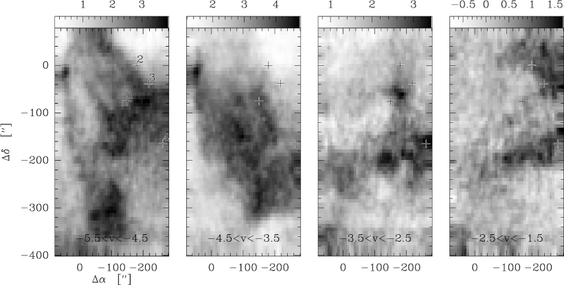
Figure 1: $\rm{}^{12}CO$(J=2–1) channel maps of the Polaris field. The 4 positions observed in $\rm HCO^{+}$ lie at offsets (-150”, -75”), (-180”, 0), (-218”, -38”), (-262”, -165”) relative to (0,0): $l_{II}=123.68$, $b_{II}=24.93$. They are indicated with crosses (positions 1 through 4 respectively). The dense core, not visible in the $\rm{}^{12}CO$ lines, is located along the eastern edge of the map, south of offset (0,0). The velocity intervals in km s^-1 are given at the bottom of each panel.

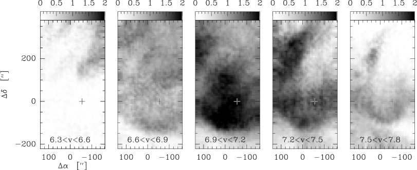
Figure 2: $\rm{}^{12}CO$(J=2–1) channel maps of the L1512 field. The position observed in $\rm HCO^{+}$ is at offset (-55”,0) relative to (0,0): RA=05h00m54.5s, Dec=32${}^{{}^{\circ}}$ 39’ (1950). The dense core is centered on the (0,0) position and is about 2 arcmin in diameter (Lee, Myers & Tafalla (2001), Pety & Falgarone (2003)). The velocity intervals in km s^-1 are given at the bottom of each panel.

Table 1: $\rm HCO^{+}$(J=1–0), $\rm{}^{13}CO$(J=1–0) and $\rm C_{2}H$(3/2-1/2) line properties derived from Gaussian decompositions. In several cases, velocity components with similar centroid and width appear in the $\rm HCO^{+}$ and $\rm{}^{13}CO$ spectra. They are labelled A, B, C, D or E depending on the strength of the lines. These are the five cases for which the analysis can be completed. The rms noise level $\sigma$ of the spectra is also given. The value of the centroid velocity increment (CVI) measured over a lag of 0.02 pc on the $\rm{}^{12}CO$(1-0) line at each position is also given.

					$\rm HCO^{+}$(J=1–0)				$\rm{}^{13}CO$(J=1–0)
	offsets		CVI		$v_{i}$	${T_{\rm A}^{*}}_{i}$	$\sigma$	$\Delta v_{i}$	$v_{i}$	${T_{\rm A}^{*}}_{i}$	$\sigma$	$\Delta v_{i}$
	”	”	km s-1		km s-1	K	mK	km s-1	km s-1	K	mK	km s-1
Polaris #1	-150	-75	0.08	D	-4.7	0.15	5	0.65	-4.7	2.	16	0.4
				D	-4.3	0.12		0.6	-4.3	2.2		0.5
				C	-3.6	0.02		0.4	-3.8	0.8		0.3
				A	-2.7	0.015		1.1	-3.4	0.14		1.1
Polaris #2	-180	0	0.4	C	-4.8	0.06	3	0.4	-4.6	0.6	11	0.5
					-4.55	0.08		0.5	-3.3	0.2		0.8
				B	-3.9	0.02		1.2	-2.9	0.2		0.8
				A	-2.9	0.01		2.0	-3.0	0.07		2.1
Polaris #3	-218	-38	0.4	C	-4.7	0.075	3	0.7	-4.7	1.5	6	0.5
				B	-4.0	0.03		1.1	-3.4	0.3		1.2
				A	-2.5	0.01		1.8	-1.9	0.09		0.9
Polaris #4	-262	-165	0.1	C	-4.6	0.05	8	1.0	-4.5	0.7	24	1.2
				C	-3.6	0.06		1.3	-3.9	1.4		1.2
				C	-3.2	0.07		0.4	-3.2	0.9		0.5
									-2.8	0.08		2.4
L1512	-55	0	0.06	E	7.0	0.5	6	0.3	7.0	3.7	50	0.2
				dc	7.2	1.7		0.15	7.2	4.4		0.3
				C	7.2	0.05		0.9	7.4	1.3		0.6
				$\rm C_{2}H$(3/2,2-1/2,1)
	offsets			$v_{i}$	${T_{\rm A}^{*}}_{i}$	$\sigma$	$\Delta v_{i}$
	”	”		km s-1	mK	mK	km s-1
Polaris #2	-180	0		-3.5	7.	3.	3.0

Four positions have been observed in the Polaris environment and one in that of L1512. They are shown in the $\rm{}^{12}CO$(J=2–1) channel maps of Figs 1 and 2, from the IRAM-30m data of Pety & Falgarone (2003). These positions sample the full range of small scale velocity shears, following the statistics of the velocity field of Pety & Falgarone (2003). The observed quantity used in such statistics is the $\rm{}^{12}CO$ line centroid velocity increment (CVI) measured for a given lag. The CVI values measured for a lag of 0.02 pc are given in Table 1 for each position. They correspond to local velocity shears (in the plane of the sky) ranging from 3 to 20 km s^-1 pc^-1, the smallest value in the Polaris field belonging to the Gaussian core of the probability distribution of the CVIs in that field, while the largest values (positions #2 and #3 in Polaris) belong to its non-Gaussian tails. The CVI value in L1512 also belong to the non-Gaussian tail of the CVI probability distribution, but is close to the limit of its Gaussian core.

2.2 Observations and results

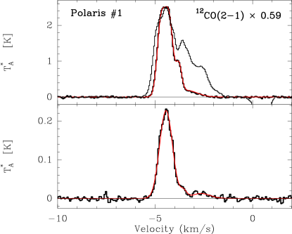
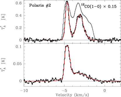
Figure 3: In each of the 4 panels, corresponding to the 4 positions observed in the Polaris field, three lines are displayed: $\rm{}^{13}CO$(J=1–0) (thick line) and a multi-component Gaussian fit (thick red curve), $\rm{}^{12}CO$ (either (J=1–0) or (J=2–1), as indicated) multiplied to fit the $\rm{}^{13}CO$ temperature scale, and the $\rm HCO^{+}$(J=1–0) at the bottom with a multi-component Gaussian fit (thick red curve).

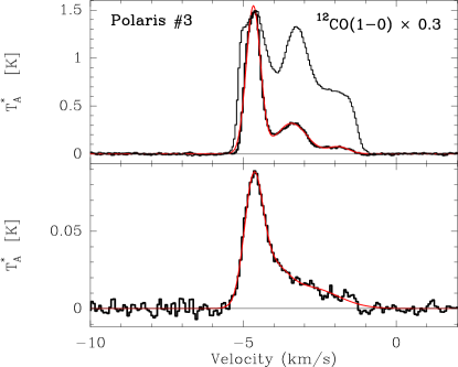
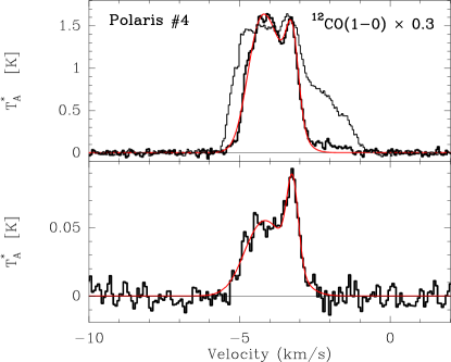
Figure 4: Same as Fig. 3 for positions 3 and 4 in Polaris.

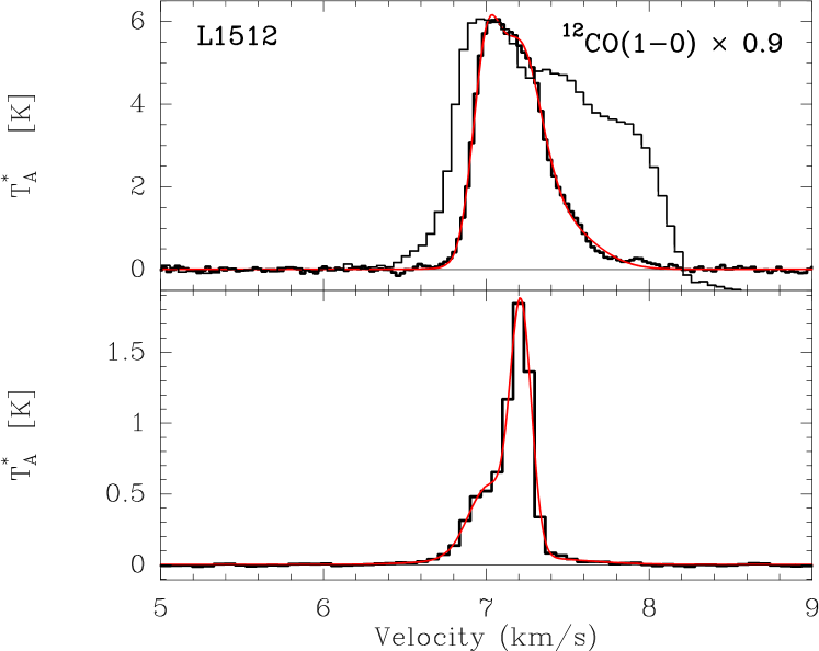
Figure 5: Same as Fig. 3 for the position in L1512. Note the very different antenna temperatures, with respect to the Polaris field, for the $\rm HCO^{+}$ line in particular, due to the fact that the dense core is sampled by the beam in L1512. The velocity scales for the two fields are also very different.

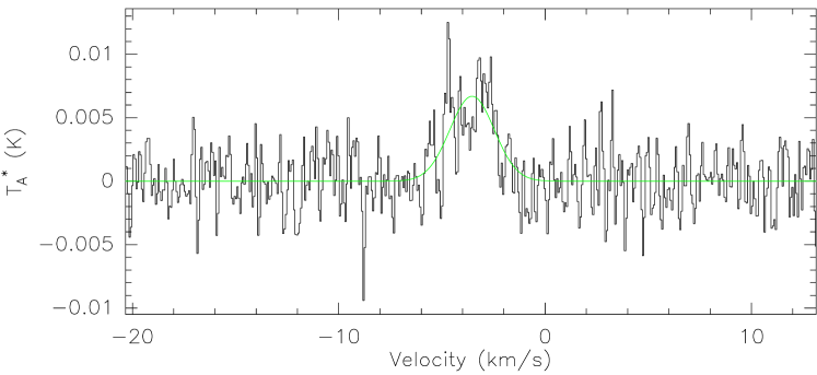
Figure 6: $\rm C_{2}H$ spectrum at position 2 in Polaris.The line parameters derived from the Gaussian fit are: $v=-3.5$km s^-1, $T_{\rm A}^{*}$=7mK, $\sigma$=3mK and $\Delta v=$3 km s^-1).

The observations were carried out at the IRAM-30m telescope and spread over three summer sessions (1996, 1998 and 1999). A few additional $\rm{}^{12}CO$ and $\rm{}^{13}CO$(J=2–1) lines have been obtained in the framework of another project during a winter session in 1999. The weather conditions never allowed us to observe at high frequency during the summers and the lines observed were $\rm HCO^{+}$(J=1–0), $\rm{}^{13}CO$(J=1–0) and C₂H(3/2-1/2). Frequency switching by 7.8 MHz was used to subtract the off line emission. The autocorrelator had a resolution of 20 kHz providing a velocity resolution of 0.08 km s^-1 at 89 GHz. The single sideband noise temperatures of the receivers greatly improved in 1999 when a new generation of receivers was installed. At 3mm, the SSB receiver temperatures were in the range 80-130 K depending on the frequency before 1999 and 50-65 K in 1999. The system temperatures were in the range 200-250 K before 1999 and between 150 and 250 K in 1999. The sideband rejections were estimated to be about 20 dB. At 230GHz, the SSB receiver temperature was about 90 K with $\approx$ 13 dB gain rejection. The $\rm HCO^{+}$(J=1–0), $\rm{}^{13}CO$(J=1–0) and $\rm{}^{12}CO$(J=2–1) line profiles are shown in Figs. 3- 6 for the five positions, as well as a unique $\rm C_{2}H$ spectrum.

In L1512, the line of sight crosses the dense core, so the spectra comprise the emission of both the dense core (the narrow component between 7.1 and 7.3 km s^-1) and that of its environment extending from 6.4 to 8.2 km s^-1. This velocity interval is assigned to the environment of the core on the basis of the line profile properties and of the large scale channel maps of Falgarone et al. (1998) and Falgarone, Pety & Phillips (2001). In Polaris, the lines of sight do not intercept the dense core therefore the observed emission is from the environment exclusively.

The exceptional signal-to-noise ratio of the line profiles reveals a large variety of complex non-Gaussian line profiles, with several broad and weak components. There is a general agreement between the total velocity extent of the CO and $\rm HCO^{+}$ lines (except for position # 4 in Polaris) but the lineshapes are all extremely different. The velocity components visible in the $\rm{}^{13}CO$ spectra are most often present in the $\rm HCO^{+}$ spectra at the same position. The $\rm HCO^{+}$ and $\rm{}^{13}CO$ lines have thus been decomposed into several Gaussians with the goal of ascribing a $\rm{}^{13}CO$(1-0) counterpart to each of the $\rm HCO^{+}$ components. The decomposition of these profiles into Gaussians is not straightforward, and certainly not unique, but it is a guidance in the analysis of the spectra. Yet, as shown in Table 1, not all the components found in the Gaussian fitting procedure of the $\rm HCO^{+}$ lines have been found successfully in that of the $\rm{}^{13}CO$ lines and vice versa. In most cases, the broad $\rm HCO^{+}$ weak emission has been fitted with a single Gaussian, although in a few cases, several narrower Gaussians would also fit to the profile.

Table 2: LVG results for the five template velocity components. ¹³CO(1-0) line: range of input values for $R$(2-1/1-0) (col. 2) and $T_{\rm A}^{*}$(1-0) (col. 3), result for the $\rm{}^{13}CO$ column density per unit velocity (col. 4). HCO⁺(1-0) line: input $T_{\rm A}^{*}$(col. 5), lower and upper values for the $\rm HCO^{+}$ column density met along the curves shown in Fig. 8 (col. 6), and corresponding range of $\rm{}^{13}CO$/$\rm HCO^{+}$ ratios (col. 7).

	$R$(2-1/1-0)	$T_{\rm A}^{*}$($\rm{}^{13}CO$)	$N({\rm{}^{13}CO})/\Delta v$	$T_{\rm A}^{*}$($\rm HCO^{+}$)	$N({\rm HCO^{+}})/\Delta v$	$N({\rm{}^{13}CO})/N({\rm HCO^{+}})$
		K	$\,{\rm cm}^{-2}$/km s-1	K	$10^{12}$$\,{\rm cm}^{-2}$/km s-1
A	0.3 – 0.6	0.07 – 0.2	1.2$\times 10^{14}$	0.01	0.1 – 0.3	1200 – 400
B	0.3 – 0.6	0.2 – 0.5	3$\times 10^{14}$	0.025	0.1 – 0.25	3000 – 1200
C	0.3 – 0.6	0.7 – 1.5	1.2$\times 10^{15}$	0.09	0.7 – 1	1700 – 1200
D	0.5 – 0.6	2. – 3.	2.$\times 10^{15}$	0.24	1.2 – 2.3	1667 – 870
E	0.55 – 0.65	5. – 7.	7.2$\times 10^{15}$	0.5	2.5 – 4.0	2880 – 1800

Figure 7: Peak antenna temperature versus half-power linewidth of all the Gaussian components identified in the $\rm HCO^{+}$(1-0) line profiles and listed in Table 1.

We have restricted our analysis of the $\rm HCO^{+}$ lines to the components which are visible in the $\rm{}^{13}CO$(1-0) spectra i.e. those for which it exists a $\rm{}^{13}CO$ counterpart with comparable centroid velocity and width. They are labelled with letters in Table 1. Instead of analysing all the profiles separately, we give outlines of the solutions by splitting the range of line temperatures into five cases (labelled by letters A to E). Each case is identified by its $\rm HCO^{+}$(1-0) temperature within a factor of the order of 3, given in Table 2. Note that in all cases but E, the $\rm HCO^{+}$/$\rm{}^{13}CO$ line temperature ratio is $\approx$ 0.1. The weakest cases are the A’s while the E case approaches the conditions within dense cores (noted ”dc” in Table 1). The characteristics of all the components are reported in Table 1. Table 1 shows that the $\rm HCO^{+}$ line temperatures range between 0.01 and 0.5 K, a range similar to that found towards $\zeta$ Oph by Liszt & Lucas (1994) and in the direction of several extragalactic sources by Lucas & Liszt (1996). An interesting rough anticorrelation appears between the $\rm HCO^{+}$ peak intensity and the width of each component where approximately ${T_{\rm A}^{*}}_{i}({\rm HCO^{+}})\propto\Delta v_{i}^{-2}$ (Fig. 7). It will be discussed in Section 4.5.

3 Column densities and abundances

3.1 $\rm HCO^{+}$

$\rm HCO^{+}$ line intensities have been interpreted in the framework of the Large Velocity Gradient (LVG) formalism. The collisional excitation due to electrons has been included in the code following Bhattacharyya, Bhattacharyya & Narayan (1981), with ionisation degrees $x_{e}=10^{-4}$ and $x_{e}=10^{-5}$. The HCO⁺–electron rates calculated by Faure & Tennyson (2001) have not been used, since they only calculate the rates up to $J=2$, while for our calculations higher excitation levels have been included. We have verified that, at least for higher temperatures, the rates from Faure & Tennyson (2001) and Bhattacharyya, Bhattacharyya & Narayan (1981) do not differ significantly. Collisional excitation of $\rm HCO^{+}$ by $\rm H_{2}$ at high temperature is implemented by using the cross-sections computed by Flower (2000). The excitation temperature, optical depth and emergent intensity in the J=1-0 transition of $\rm HCO^{+}$ have been computed for $\rm H_{2}$ densities ranging between 30 and $10^{5}$ $\,{\rm cm}^{-3}$ and kinetic temperatures $T_{k}=10$ and 250 K. Temperatures as large as 250 K have been considered because observations of the $\rm{}^{12}CO$(J=3–2) and J=4–3 transitions of a few positions in the environment of L1512 reveal $\rm{}^{12}CO$ intensities larger in these transitions than anticipated from the low J lines if the gas is cold and dense. Diluted ($n_{{\rm H_{2}}}=200{\,{\rm cm}^{-3}}$) and warm ($T_{k}=250$ K) gas is a possible solution (Falgarone, Pety & Phillips 2001). An upper limit $T_{k}=200$ K on the kinetic temperature is provided by the width of the $\rm HCO^{+}$ velocity components, whose median value is 0.6 km s^-1. At $T_{k}=200$ K, the thermal velocity of $\rm HCO^{+}$ is only $v_{th}=0.24$ km s^-1, and the thermal contribution to the linewidth $\Delta v_{th}=0.57$ km s^-1.

Although weak, the $\rm HCO^{+}$ lines are not optically thin throughout the intensity range 0.01-0.5 K. For densities lower than a few 10³ $\,{\rm cm}^{-3}$, the optical depth approaches unity, as the excitation temperature drops towards the Cosmic Background temperature. To break the degeneracy of the problem, we use the $\rm{}^{13}CO$(J=1–0) and J=2-1 lines to constrain the $\rm H_{2}$ density and temperature domain of the solutions and, as said above, we restrict our analysis to those components of similar kinematic characteristics in the $\rm HCO^{+}$ and $\rm{}^{13}CO$ spectra. The $\rm{}^{13}CO$ lines are optically thin (or almost thin, in the case of L1512) so that the column density per velocity unit is well determined and the two constraints of the $\rm{}^{13}CO$(J=1–0) antenna temperature and $R$(2-1/1-0) line ratio define a narrow track of solutions in the density-temperature plane, which nevertheless spans the whole range from cold/dense to warm/diffuse gas. Each [$\rm HCO^{+}$, $\rm{}^{13}CO$] pair of components (i.e. each letter in Col. 4 of Table 1) has then to be interpreted with the set of values ($n_{{\rm H_{2}}},T_{k}$) allowed by the $\rm{}^{13}CO$ lines. This method provides determinations of the $\rm HCO^{+}$ column density per unit velocity $N({\rm HCO^{+}})/\Delta v$ that do not suffer from the lack of knowledge of the density, a critical parameter for a line so difficult to excite. The results for each ($n_{{\rm H_{2}}},T_{k}$) set are displayed in Fig. 8, where the labels on the curves indicate the gas kinetic temperature, given only once on the upper curve. The tracks appear on that figure, from $\rm H_{2}$ densities in the range 1–2$\times 10^{3}$ $\,{\rm cm}^{-3}$ at temperatures below 15 K and to densities between 100 and 300 $\,{\rm cm}^{-3}$ at temperatures above 100 K. In the following discussion, we restrict the domain of $T_{k}$ to a range 15 – 20 K to 200 K, the lower value being the temperature of a gas of density 1 – 2$\times 10^{3}$ $\,{\rm cm}^{-3}$, shielded from the solar neighbourhood UV field by 0.5 to 1 mag (Le Petit, Roueff & Herbst (2004)), the upper limit corresponding to a fully thermal contribution to $\rm HCO^{+}$ line widths of 0.57 km s^-1.

Figure 8: $\rm HCO^{+}$ column densities per unit velocity as a function of $\rm H_{2}$ density, for the five template components (A to E) for which the LVG analysis is possible (see text). Six values of the kinetic temperature are given along the upper curve, the same values being marked by the 6 symbols on the other curves. Each ($n_{{\rm H_{2}}},T_{k}$) set belongs to the narrow track of solutions allowed by the CO data (Sect. 3).

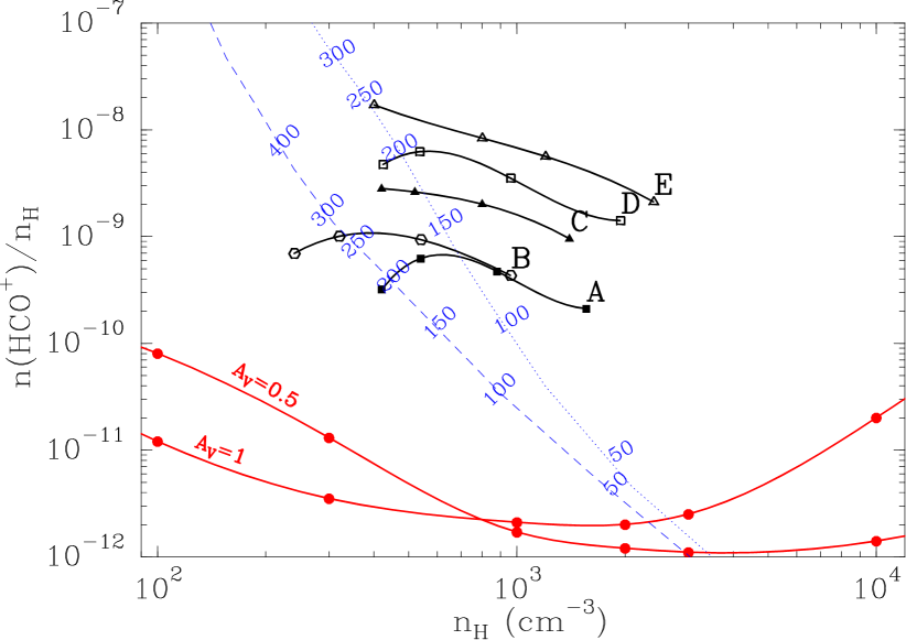
Figure 9: $\rm HCO^{+}$ abundances as a function of the hydrogen nuclei density. The five upper curves (thick solid curves) are the tracks derived from the observations displayed with the same symbols as in Fig. 8. The kinetic temperature varies along each curve and the symbols are located at $T_{k}=$20, 40, 100 and 200 K from right to left. The ($n_{\rm H},T_{k}$) sets are those inferred from the CO data. Thick lower curves (red): Results of steady-state chemistry models, computed for two different values of the UV shielding, $A_{v}=0.5$ and 1 mag. Dashed and dotted curves (blue): Tracks of non-equilibrium chemical computations along two isobaric cooling sequences (see Section 4.4). The initial conditions are the same ($n_{\rm H}=100$ $\,{\rm cm}^{-3}$) except for the shielding from the ISRF: $A_{V}=0.2$ mag (dashed) and $A_{V}=1$ mag (dotted). On each of them, the gas temperature decreases from top to bottom and is given along each track to allow a comparison of the LVG and chemical solutions in the [$X({\rm HCO^{+}}),n_{\rm H},T_{k}$] space.

In spite of the large range of kinetic temperatures considered, $20<T_{k}<200$ K, Fig. 8 shows that the $\rm HCO^{+}$ column density of each component is determined to within a factor of a few (see also Table 2). Their values for the ensemble of the five template components span more than one order of magnitude.

The main difficulty in the derivation of the $\rm HCO^{+}$ abundances from the above set of column densities, is the estimate of the relevant hydrogen column density of each component. This is so because each component is defined only by its velocity and velocity width and contributes to only a small fraction of the total column density. In the following expression of the $\rm HCO^{+}$ abundance:

$$X({\rm HCO^{+}})={\left(N({\rm HCO^{+}})\over\Delta v\right)}\Delta v{1\over n_{\rm H}\,L}$$ (1)

$N({\rm HCO^{+}})\over\Delta v$ and $n_{\rm H}$ are derived from the above LVG analysis for each case, $\Delta v$ is known from the data. Here, $n_{\rm H}=2n_{{\rm H_{2}}}$ is the density of protons in a gas where the density of atomic hydrogen has been neglected, according to PDR models for gas with UV shieldings above 0.2 mag (Le Petit, Roueff & Herbst (2004)). The depth $L$ is the only independent, unknown and free parameter in the derivation of $X({\rm HCO^{+}})$. An estimate of the depth $L$ is thus needed for each velocity component. The channel maps in the $\rm{}^{12}CO$(J=2–1) lines (Figs. 1 and 2) have been used to estimate the spatial extent in projection, $L$, of each of the velocity components. The similarity of the velocity coverages of the $\rm{}^{12}CO$ and $\rm HCO^{+}$ lines suggests that at the scale of the resolution these species are well mixed in space too. The lengthscale $L$ characteristic of the structures are all of the order of 0.05 pc in projection. The actual lengthscale over which the line forms may be longer by a factor of a few, less than 10 on statistical grounds (then the filaments would be the edge-on projection of sheets) or smaller if substructure exists. In the following, we adopt $L=0.1$ $\,{\rm pc}$ for all the components. Note that the estimated total column density of individual velocity components thus ranges from $N_{\rm H}=7.5\times 10^{19}$ $\,{\rm cm}^{-2}$ to ten times more, or $0.04<A_{V}<0.4$, smaller, as expected, than the cloud visual opacities discussed in Sections 2 and 4.2. A velocity coverage $\Delta v=0.5$ km s^-1 has been adopted for all the components as the median value of the well-identified components in Table 1. The broadest components are likely collections of narrower sub-components. The results are shown in Fig. 9 for the five cases analysed. The symbols are the same as in Fig. 8 and on each curve they mark the set of kinetic temperatures, $T_{k}=$20, 40, 100 and 200K from right to left. According to the previous discussion, these abundances may have been over or underestimated by a factor 3 at most. We compare these determinations to results of chemical models in Section 4.

3.2 $\rm C_{2}H$

The width of the $\rm C_{2}H$ line is large and probably corresponds to the weakest component seen in the $\rm HCO^{+}$ profile at the same position (case A). With one transition detected only, one can simply estimate the column density assuming the excitation temperature and low opacity. For $A_{3/2,2-1/2,1}=4.1\times 10^{-7}$ s^-1 and an excitation temperature of 10 K, the inferred column density is $N({\rm C_{2}H})=2\times 10^{12}$ $\,{\rm cm}^{-2}$. The corresponding abundance, is $X({\rm C_{2}H})=2\times 10^{-8}$ for an estimated total column density $N_{\rm H}\approx 10^{20}$ $\,{\rm cm}^{-2}$ from $n_{\rm H}\approx 500{\,{\rm cm}^{-3}}$ (Fig. 9) and $L=0.1$ pc.

At this position, the same component has $N({\rm HCO^{+}})=3\times 10^{11}$ $\,{\rm cm}^{-2}$, which makes this component similar to the weakest lines detected by Lucas & Liszt (2000) in diffuse molecular clouds with the PdBI, with an abundance ratio $\rm C_{2}H$/$\rm HCO^{+}$$\approx 7$, consistent with the non-linear relationship they find between these two species.

4 Comparison with chemical models

4.1 Description of the steady-state model for chemistry

Steady-state $\rm HCO^{+}$ abundances have been computed using the Meudon PDR code . Models here consider semi-infinite clouds of constant density in plane-parallel geometry with ionizing photons coming from one side. The UV spectral density of the photons is scaled according to the Draine radiation field (Draine (1978)). The dust extinction curve is the galactic one as parameterized by Fitzpatrick & Massa (1990). The computation proceeds from the exterior and penetrates into the cloud. At each step, chemical and thermal equilibrium are reached self-consistently. Radiative cooling makes use of the on-the-spot approximation which considers that an emitted photon is either re-absorbed locally or escapes from the cloud, and line emissivities depend on the abundances. Radiative transfer into lines of $\rm H_{2}$ and CO is computed using the approximation of Federman, Glassgold & Kwan (1979). The depth into the cloud is measured in magnitudes of visual extinction ($A_{V}$). Therefore, $A_{V}=0$ mag at the edge of the illuminated cloud, increasing when moving deeper into it. One is then free to consider some particular points into the cloud, corresponding to particular visual extinctions. We have computed the abundance of $\rm HCO^{+}$ in several models with different hydrogen densities, and plot the result at two depths in the cloud, $A_{V}=0.5$ and 1 mag (see figure 9). Since the total extinction in the direction of the observed positions is smaller than 1 mag (see Section 2.1) except for the gas in the L1512 dense core, not under consideration here, it is reasonable to assume that locally the UV shielding is also less than 1 mag, hence the two PDR cases shown in Fig. 9.

4.2 Lack of steady-state chemical solutions

Fig. 9 shows that none of the $\rm HCO^{+}$ abundances derived from the observations are consistent with steady-state chemistry in clouds moderately shielded from the ambient UV field, even at high density. The uncertainties in the abundance derivations are large and due mostly to the unknown extent of the emitting gas along the line of sight $L$. Note, however, that a depth 10 to 100 times larger (i.e. 1 to 10 pc) would be required to bring the curves deduced from the observations down to the domain of steady-state solutions. Depths larger than $\sim$ 3pc are ruled out by the average column density in the fields, $A_{V}<1$. Structures smaller than 0.1 pc are indeed suggested by the PdBI observations reported in Paper III. We thus conclude that the observed $\rm HCO^{+}$ abundances cannot be produced by state-of-the-art models of gas phase steady-state chemistry in diffuse molecular clouds.

4.3 Non-equilibrium chemistry

An alternative scenario relies on the proposal that small regions bearing chemical signatures different from those of the bulk of gas are permanently generated in interstellar matter by bursts of dissipation of turbulence. The space-time intermittency of turbulence dissipation is such that the heating rate due to the local release of suprathermal energy may exceed those driven by the UV radiation field. In low density gas and in the UV field of the Solar Neighborhood, it is the case as soon as dissipation is concentrated in less than a few % of the volume (see the review of Falgarone (1999)).

Intermittent dissipation locally heats the gas far above its average equilibrium temperature, over a timescale sufficient to trigger a specific chemical network driven by endothermic reactions or involving large activation barriers. In the regions heated by non-thermal energy from turbulence, the endothermic barrier ($\Delta E/k$ =4640 K) of the $\rm C^{+}$ + $\rm H_{2}$ $\rightarrow$ $\rm CH^{+}$ + H reaction is overcome and it occurs at a much higher rate than the slow radiative associations, $\rm C^{+}$ + H $\rightarrow$ $\rm CH^{+}$ + $h\nu$ and $\rm C^{+}$ + $\rm H_{2}$ $\rightarrow$ $\rm CH_{2}^{+}$ + $h\nu$ (Black, Hartquist & Dalgarno (1978)). Such a scenario was first suggested by the good observed correlation between $\rm CH^{+}$ column densities and rotationally excited $\rm H_{2}$ (Lambert & Danks (1986)). The $\rm CH^{+}$ ions then initiate the hydrogenation chain, $\rm CH^{+}$ + $\rm H_{2}$ $\rightarrow$ $\rm CH_{2}^{+}$ + H and $\rm CH_{2}^{+}$ + $\rm H_{2}$ $\rightarrow$ $\rm CH_{3}^{+}$ + H, which does not proceed further because $\rm CH_{3}^{+}$ recombines with electrons faster than it reacts with $\rm H_{2}$. In the regions heated by non-thermal bursts of energy, $\rm CH_{3}^{+}$ thus becomes the most abundant ion. As discussed in the specific model of JFPF, it is even more abundant than $\rm CH^{+}$ because its formation rate stays larger than its destruction rate. It opens a new route of formation for $\rm HCO^{+}$,

$${\rm CH_{3}^{+}}\ +{\rm O}\rightarrow{\rm HCO^{+}}\ +{\rm H_{2}}.$$ (2)

Large amounts of $\rm HCO^{+}$ are thus expected to be produced by this chemistry, even in regions weakly shielded from the UV field. There, $\rm HCO^{+}$ is, in part, a daughter molecule of $\rm CH^{+}$, although other routes are also active (see Section 5).

Following Moffatt, Kida & Ohkitani (1994), the regions of intermittent dissipation have been modeled in JFPF by Burgers vortices threaded by helical magnetic fields, an alternative scenario to magneto-hydrodynamic (MHD) shocks in the absence of obvious post-shock compressed layer. The vortex is fed by large scale motions. Its lifetime is therefore the turnover time at of these large scales, of the order of ten times (or more) its own period, $P$. Therefore, the characteristics of the vortex are not free parameters but imposed by the ambient turbulence. Viscous dissipation is concentrated in the layers of large velocity shear at the edge of the vortex. In magnetized vortices of the CNM, JFPF show that decoupling occurs between the neutrals spiralling in and the ions tightly coupled to steady helical fields. An additional local heating rate, due to the friction between the ions and the neutrals, is thus present. The chemistry in the diffuse gas reacts swiftly to the sharp increase of gas temperature generated by turbulence dissipation. In the model of JFPF, relevant for the CNM, the period of the vortex is $P=600$ yr, its lifetime $\approx 10^{4}$ yr, and the minimum time to build up the molecular abundances specific of the warm chemistry is $t_{warm}\approx 200$ yr.

The sequence of events we consider is therefore: diffuse gas enters such a vortex (or an ensemble of vortices braided together), spiralling inward. It is heated and enriched chemically during at least 200 yr while it crosses the layers of largest velocity shear and largest ion-neutral drift, the active layers of the vortex. Then it enters the central regions of the vortex where the temperature drops due to the decrease of dissipation. The gas formerly heated and chemically enriched, starts cooling down and condensing self-consistently with chemistry. Its radial velocity there has become vanishingly small. Eventually, the vortex blows-up, after $\approx 10^{4}$ yr.

The thermal and chemical evolution of the gas in the active warm layers of the vortex has been computed in JFPF. Here, we follow the time-dependent evolution of the density, temperature and chemical abundances of the gas, once it has left these active layers. An isobaric evolution is assumed. We use another code with the same chemical network and the same cooling functions. The time-dependent evolution is computed for a given and constant shielding from the UV field. The gas temperature is derived from the radiative cooling rate which depends on the chemical abundances, the $\rm H_{2}$ density and temperature.

The results are displayed in Fig. 10 for four different initial conditions in density and shielding from the UV field. Two initial densities are considered $n_{\rm H}=30$ and 100 $\,{\rm cm}^{-3}$, representative of the cold neutral medium (CNM). The local heating rate due to turbulent dissipation, $\Gamma_{d}$, characterizes the strength of the burst. Two values have been chosen, $\Gamma_{d}=10^{-21}$ $\,{\rm erg}\,{\rm cm}^{-3}{\rm s}^{-1}$ for the densest case and $\Gamma_{d}=10^{-23}$ $\,{\rm erg}\,{\rm cm}^{-3}{\rm s}^{-1}$ for the other, so that the initial kinetic temperature is close to 10³ K in each case. These values correspond to the average heating rate due to turbulence dissipation in the CNM, ${\overline{\Gamma}_{d}}=2\times 10^{-25}({\overline{n}}_{\rm H}/30{\,{\rm cm}^{-3}})$ $\,{\rm erg}\,{\rm cm}^{-3}{\rm s}^{-1}$, divided by the estimated volume filling factor of the gas affected by the burst, or $\approx 2\times 10^{-2}$ for the weaker type of burst and $\approx 10^{-3}$ for the stronger and therefore rarer type (see the discussion in JFPF and Falgarone (1999)). Two values of the shielding from the ambient ISRF are also considered $A_{V}=$ 0.2 and 1 mag to bracket the conditions prevailing in the gas under study. The ionisation degree stays close to $x_{e}=10^{-4}$ along the isobaric evolution at $A_{V}=$ 0.2 and varies between $x_{e}=10^{-4}$ and $10^{-5}$ in the other case, following the chemical evolution of the ions. These upper and lower values of $x_{e}$ are those used in the LVG code. The initial chemical abundances are those produced by the warm chemistry in the active layers of the vortex, as computed by JFPF.

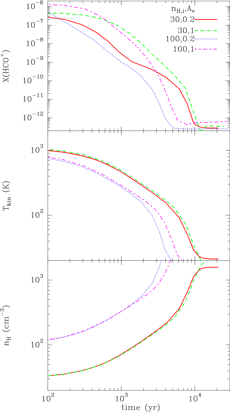
Figure 10: Time-dependent evolution of (top) the $\rm HCO^{+}$ abundance, (middle) the kinetic temperature and (bottom) the hydrogen density, along the isobaric cooling of a parcel of gas formerly enriched chemically in a burst of dissipation of turbulent energy. The initial densities are $n_{{\rm H},i}$ =30 (dashed and solid) and 100 $\,{\rm cm}^{-3}$ (dotted and dot-dashed), and the shieldings from ISRF are $A_{V}=$ 0.2 (solid and dotted) and 1 mag (dashed and dot-dashed)

It is remarkable that the signatures of the warm chemistry are kept by the gas for more than 10³ years after the gas has escaped the active layers. The curves of Fig. 10 illustrate the marked non-linearity of the chemical evolution: (1) large differences are visible after only 10³ years between the tracks followed by two parcels of gas with very similar initial conditions, (2) the drop of $X({\rm HCO^{+}})$ is by 6 orders of magnitude while the density and temperature vary by a factor 50 only.

4.4 Existence of [$X({\rm HCO^{+}}),n_{\rm H},T_{k}$] tracks crossing the observation domain

We show below that we may have detected the decaying signatures of the warm chemistry generated by bursts of dissipation of turbulence. The time-dependent evolution of an enriched parcel of gas once the heating due to dissipation of turbulence has dropped, is a curve in the [$X({\rm HCO^{+}}),n_{\rm H},T_{k}$] space which depends on the initial conditions and UV shielding (see Fig. 10). It is therefore not straightforward to compare it with observational results. As an illustration that such an evolution is consistent with our data, we have drawn two of the tracks of Fig. 10 (those corresponding to the largest initial density) in the [$X({\rm HCO^{+}})$–$n_{\rm H}$] plane of Fig. 9. On each of them, the gas temperature decreases from top to bottom from about 500 to 50 K. In that plane, the LVG solutions and the cooling tracks are almost perpendicular. The only temperature range where they are consistent are over the range 100–300 K: the low extinction track (dashed curve) is consistent with the LVG solutions for components A and B and the more shielded evolution (dotted curve) for all the others (C, D and E).

Table 3: Sets of non-equilibrium $\rm HCO^{+}$ abundances consistent with $\rm HCO^{+}$(J=1–0) line observations. Each solution is given as a range of values for the set [$X({\rm HCO^{+}}),n_{\rm H},T_{k}$] corresponding to the range of observed values (cases A to E). The parameters of the models are the turbulent heating rate $\Gamma_{d}$, the shielding from the UV field $A_{v}$ and the initial density $n_{{\rm H},i}$.

$\Gamma_{d}$	$A_{v}$	$n_{{\rm H},i}$	$X({\rm HCO^{+}})$	$n_{\rm H}$	$T_{k}$
erg cm-3 s-1		$\,{\rm cm}^{-3}$		$\,{\rm cm}^{-3}$	K
10-21	0.2	100	8–2 $\times 10^{-10}$	320–500	250–150
10-21	1	30	3–0.5$\times 10^{-9}$	130–200	250–170
10-21	1	100	6–1.6$\times 10^{-10}$	700–900	150–120
10-23	0.2	30	9–3$\times 10^{-9}$	80–130	250–160
10-23	1	100	7–1$\times 10^{-9}$	100–120	250–220

The range of values of the $\rm HCO^{+}$ abundances, density, kinetic temperature of the part of the isobaric cooling consistent with the observations (cases A to E) are given in Table 3 for five different sets of initial conditions, including the strength of the dissipation burst which determines the local heating rate, $\Gamma_{d}$.

We have not explored a larger domain of initial conditions because our goal here is only to illustrate the compatibility of such a non-equilibrium chemistry with the data. A more detailed analysis requires further constraints to treat the many non-linearities of the physics and chemistry involved and explore a relevant part of the vast parameter space. Moreover, our model, although complex in terms of coupled processes, is still too crude. For instance, we have neglected the initial dynamical expansion of the warm gas because the radiative cooling and chemical timescales, up to $\sim$ a few thousand years, are smaller than the expansion time of the warm gas under the effect of pressure gradient, just after the burst of dissipation. The timescale for a warm structure of initial thickness $L_{0}$ to double its size under expansion at the sound velocity in the ambient cold neutral medium ($c_{S}\sim 0.5$ km s^-1) is 2$\times 10^{5}(L_{0}/0.1{\,{\rm pc}})$ yr. Would they be much smaller, the timescale would be shorter. The Lorentz force acting on the ions somewhat delays the expansion at a rate which depends on the gas ionisation degree and geometry of the helical magnetic fields.

Nonetheless, the above comparison brings to light a few interesting results: all the solutions provided by the non-equilibrium chemistry consistent with the observations are warmer than 100 K (Table 3) and the inferred $\rm HCO^{+}$ abundances are all larger than $2\times 10^{-10}$ and as large as $\approx 10^{-8}$. They are more than one order of magnitude above the values computed at steady-state at densities less than $10^{3}$ $\,{\rm cm}^{-3}$. It is remarkable that these abundances bracket the value $X({\rm HCO^{+}})=2\times 10^{-9}$ determined by Lucas & Liszt (1996) and Liszt & Lucas (2000) from their observations of the $\rm HCO^{+}$(J=1–0) line in absorption against extragalactic continuum sources. These lines of sight sample ordinary interstellar medium of low visual extinction (many of the extragalactic background sources are visible QSOs) as opposed to dense cores and star forming regions. It is thus plausible that their observations sample the kind of molecular material we discuss here, their inferred abundances being an average along the lines of sight of $\rm HCO^{+}$-poor and $\rm HCO^{+}$-rich regions. Last, results are weakly sensitive to the strength of the dissipation burst, as if the actual initial conditions were rapidly forgotten.

4.5 The $\rm HCO^{+}$ enrichment and the strength of the velocity shear

As seen in Table 1, the five observed positions do not sample gas with similar kinematic properties: two positions (Polaris # 2 and 3) lie on the locus of largest velocity shears in the Polaris field (i.e. populating the non-Gaussian tails of the probability distributions of CVIs, Pety & Falgarone (2003)). The others correspond to smaller velocity shears. Against all expectation (Table 1), the largest $\rm HCO^{+}$ abundances (D, E and dc components) are found at those positions of smallest CVIs, while the set of least chemically enriched components (A, B and C) are found at the positions with the largest CVIs. Since the larger the velocity shear, the larger the dissipation and heating rates and the gas temperature, one expects that the chemical enrichment would increase with the velocity shear or the CVIs, but it is not what is observed.

These results suggest a broader time sequence, encompassing that discussed in the previous section, in which the increase $\rm HCO^{+}$ abundance is a measure of the elapsed dissipation: the longer the dissipation has been going on, the smaller the velocity shear (i.e. the vortex is fading) and the larger the quantity of chemically enriched gas produced. Such a sequence is also suggested by the rough anticorrelation displayed in Fig. 7. The $\rm HCO^{+}$ column density of each component being close to ${T_{\rm A}^{*}}_{i}\Delta v_{i}$, since the line is not very optically thick, it increases as the velocity dispersion decreases, as $\Delta v_{i}^{-1}$. The observed quantity of chemically enriched gas is produced at the expense of the non-thermal kinetic energy, traced by $\Delta v_{i}$.

5 Discussion and perspectives

5.1 The complex space-time average hidden in the observed $\rm HCO^{+}$ emission lines.

The results of the last section seem to be in contradiction with the relaxation scenario described above, in which the $\rm HCO^{+}$ abundance decreases with time. Another, probably related question, is: Why, in regard of the six orders of magnitude spanned by the $\rm HCO^{+}$ abundance in the proposed non-equilibrium evolution, the observations in emission point to a much narrower range of abundances, $2\,10^{-10}<X({\rm HCO^{+}})<10^{-8}$?

This may be understood in a framework in which, several phases of the evolution are present simultaneously in the beam, for individual vortices much thinner than the beamsize, here 0.015 pc (or $\approx 3000$ AU) while vortices, in the JFPF model, have a radius $\approx 15$AU. Observations sample a mixture of gas: the most diluted and $\rm HCO^{+}$-rich, still in the warm active layers of the vortices, as long as the vortex is alive, gas already out of the warm active layers and relaxing, up to the densest, $\rm HCO^{+}$-poor gas. The older the burst, the larger the amount of relaxed gas. The signal detected in emission is sensitive to a combination of the $\rm HCO^{+}$ column density, or simply the abundance $X(t)$ assuming the total gas column density being processed is constant with time, the density $n_{\rm H}(t)$ that enters the line excitation and a term involving the duration of the phase, $\approx t$, given the broad range of timescales involved. We have computed the time integral of $X(t)\,n_{\rm H}(t)$, taken as a template for the signal in emission, assuming that we observe all the phases in the gas accumulated during at least $\approx 10^{4}$ yr, the lifetime of the vortex. For all the cases, this quantity increases linearly with time up to a maximum at about $10^{3}$ yr and does not increase further. The observations in emission are thus likely to be most sensitive to the the relaxation phase because it lasts longer and involves denser gas than the brief phase of chemical enrichment in gas too diluted to significantly excite the $\rm HCO^{+}$(1-0) line.

At the opposite, density does not weight the observations in absorption. The warmest and richest phase of the evolution, may have been detected by Liszt & Lucas (2000) as the broad and weak absorption seen in the direction of B0355+508 over the whole velocity extent of the H I absorption line.

More detailed comparison between abundances inferred from observations in absorption and in emission involves time and space averages which cannot be achieved at this stage of the study. The present observations have been obtained on one single ensemble of such dissipative structures, possibly generated simultaneously. Thus, space/time average is likely more simple than that required to interpret absorption measurements that sample depths of gas at parsec scales.

5.2 Further support for non-equilibrium chemistry: ”warm” molecules abundance ratios

The present work stresses the need for a non-equilibrium mechanism to explain the large abundances of $\rm HCO^{+}$ detected in gas of moderate density and low shielding from the ambient ISRF. In this scenario, the gas is driven locally past a high temperature threshold by an impulsive release of turbulent energy. Once the gas has escaped the region of large dissipation, it cools down and condenses and the chemistry evolves accordingly.

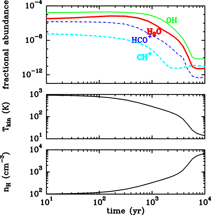
Figure 11: Time-dependent evolution of (top) the OH (thin solid), $\rm H_{2}O$ (thick solid), $\rm HCO^{+}$ (dashed), and $\rm CH^{+}$ (thin dashed) abundances, (middle) the kinetic temperature and (bottom) the total hydrogen density, along the isobaric cooling of a parcel of gas formerly enriched chemically in a burst of dissipation of turbulent energy. The initial conditions here are $n_{{\rm H},i}$ =100 $\,{\rm cm}^{-3}$, $\Gamma_{d}=10^{-21}$ $\,{\rm erg}\,{\rm cm}^{-3}{\rm s}^{-1}$ and the shielding from ISRF $A_{V}$=1.

Figure 12: Time-dependent evolution of abundance ratios, OH/$\rm HCO^{+}$ (thick), $\rm H_{2}O$/OH (thin) and $\rm CH^{+}$/$\rm HCO^{+}$ (thick dashed), along the same isobaric cooling as in Fig. 11.

Our results are independent of the details of the processes at the origin of the warm chemistry. Flower & Pineau des Forêts (1998) and Gredel, Pineau des Forêts & Federman (2002) have shown that slow MHD shocks of velocities $V_{s}\sim 10$ km s^-1 reproduce the OH/$\rm HCO^{+}$ abundance ratios observed in the diffuse medium (Lucas & Liszt (1996)). In MHD shocks, as in magnetized coherent vortices, gas is temporarily heated to temperatures as large as $10^{3}$ K. The triggered warm chemistry is characterized by coexisting large abundances of OH, H₂O, $\rm HCO^{+}$ and $\rm CH^{+}$, water and $\rm HCO^{+}$ being daughters of OH and $\rm CH^{+}$, respectively (JFPF). Their time-dependent evolution in the relaxation phase, is displayed in Fig. 11 for one of the cases discussed in Section 4 (initial density $n_{{\rm H},i}=100$ $\,{\rm cm}^{-3}$, $\Gamma_{d}=10^{-21}$ $\,{\rm erg}\,{\rm cm}^{-3}{\rm s}^{-1}$ and $A_{V}=1$). The abundance ratios along this evolution are interesting in their marked differences (Fig. 12). The $\rm H_{2}O$/OH ratio varies by less than a factor 3 along the time-dependent evolution and up to $10^{3}$ yr after the beginning of the relaxation, stays close to the values found in diffuse molecular clouds by the SWAS satellite (Neufeld et al. (2002), Plume et al. (2004)). The OH/$\rm HCO^{+}$ ratio varies by more than a factor 10 along the same evolution. We note however that its variations bracket the average value OH/$\rm HCO^{+}$$\sim$ 30 found by Lucas & Liszt (1996) in their random sampling of the diffuse ISM provided by their absorption lines survey towards extragalactic sources. In contrast, the $\rm CH^{+}$/$\rm HCO^{+}$ ratio varies very little, before $10^{3}$ yr only. The value of the ratio, though, critically depends on the density (JFPF). This follows from the fact that in our model of warm chemistry, $\rm HCO^{+}$ is not only a daughter molecule of $\rm CH^{+}$. It also forms via other routes such as CO⁺ + $\rm H_{2}$ $\rightarrow$ $\rm HCO^{+}$ + H, triggered by the endothermic charge exchange between $\rm H^{+}$ and O ($\Delta E/k=227$ K), and $\rm H_{3}^{+}$ + CO $\rightarrow$ $\rm HCO^{+}$ + $\rm H_{2}$, also slightly enhanced in warm chemistry because both CO and $\rm H_{3}^{+}$ have increased abundances in the warm layer of the vortex. This route may even be a dominant formation scheme for $\rm HCO^{+}$, if the large abundance of $\rm H_{3}^{+}$ detected on the line of sight towards $\zeta$ Per by McCall et al. (2003) happens to be the rule in the diffuse ISM.

There is also an efficient channel to form $\rm C_{2}H$ in the warm chemistry. It proceeds via the endothermic reaction ($\Delta E/k=1760$ K) CH + $\rm H_{2}$$\rightarrow$ $\rm CH_{2}$ + H, followed by a series of fast reactions: $\rm C^{+}$ + $\rm CH_{2}$ $\rightarrow$ $\rm C_{2}H^{+}$ + H, the hydrogenation of $\rm C_{2}H^{+}$ into $\rm C_{2}H_{2}^{+}$  the recombination of $\rm C_{2}H_{2}^{+}$ and terminating with photodissociation of $\rm C_{2}H_{2}$ which provides $\rm C_{2}H$.

These results are encouraging and suggest that impulsive chemical enrichment of the CNM by turbulence dissipation bears observable signatures up to several 10³ yr after the end of the enrichment.

5.3 Large scale signatures of small scale activity.

Other signatures, independent of chemistry, have been found for the existence in the CNM of gas at a few hundred Kelvin. They comprise collisional excitation of $\rm H_{2}$ far from UV sources susceptible to generate fluorescence (Gry et al. (2002); Lacour et al. (2005); Falgarone et al. (2005)). In the former cases, $\rm H_{2}$ is detected in UV absorption against nearby late B stars, in the third case, the pure rotational lines of $\rm H_{2}$ have been observed along a long line of sight across the Galaxy avoiding star forming regions. The rotational temperature of the warm $\rm H_{2}$ in these data is 276 K. In all cases the fraction of warm $\rm H_{2}$ in the total column of gas sampled is the same, of the order of a few percent. It is the same fraction as that required in the Solar Neighbourhood to reproduce the large observed abundances of $\rm CH^{+}$ within the CNM (JFPF). A few percent of warm gas, for which UV photons cannot be the sole heating source, is ubiquitous in the cold diffuse medium.

Last, we would like to stress the spatial scales presumably involved in the framework of the existing model, where individual vortices have transverse hydrogen column densities as small as $N_{\rm H}\approx 2\times 10^{16}$$\,{\rm cm}^{-2}$ corresponding to initial values $n_{\rm H,i}=100$$\,{\rm cm}^{-3}$ and $l_{i}=15$AU (JFPF). We illustrate the point with the solutions of case C: $N({\rm HCO^{+}})\approx 8\times 10^{11}$$\,{\rm cm}^{-2}$, $X({\rm HCO^{+}})\approx 2\times 10^{-9}$, $n_{H}\approx 500$$\,{\rm cm}^{-3}$. The total hydrogen column density of observed material is thus $N_{\rm H}=N({\rm HCO^{+}})/X({\rm HCO^{+}})=4\times 10^{20}$$\,{\rm cm}^{-2}$, corresponding to 2$\times 10^{4}$ vortices in the IRAM beam (here we assume that the isobaric evolution occurs at constant mass, so that the transverse column density of vortices remains the same). For the gas at 500$\,{\rm cm}^{-3}$, the transverse size has a thickness of about 3 AU. The ensemble of the 2$\times 10^{4}$ vortices, probably braided together, as vortex tubes do e.g Porter, Pouquet & Woodward (1994), would form an elongated structure about 450 AU thick, if the vortices are in contact with one another. The IRAM beam at the distance of the sources is a few times larger and the size of the structure seen with the PdBI is of this order of magnitude (Paper III). This rough estimate just shows that the existence of chemical inhomogeneities at AU scales is not ruled out in the diffuse ISM. It would certainly help understanding the remarkable similarity of the OH and $\rm HCO^{+}$ absorption line profiles reported by Liszt & Lucas (2000).

Chemical and thermal relaxation timescales are so short compared to the dynamical lifetime of molecular clouds (of at least a million year) that all the stages of the above evolution should co-exist along a random line of sight. At present, the receiver sensitivity and the telescope beam sizes provide, when observed in emission, a signal which is the space and time average of myriads of small unresolved structures, likely caught at different epoch in their evolution. Molecular line observations in absorption in the UV, visible and now submm domains are much more sensitive and have presumably already started to sample this apparently untractable complexity.

6 Summary

This work is part of a broad study dedicated to those singular regions in the environment of low mass dense cores, characterized by non-Gaussian velocity shears in the statistics of the turbulent velocity field of the clouds. These regions have been proposed to be the sites of intermittent dissipation of turbulence in molecular clouds, and the large local release of non-thermal energy in the gas there has been shown to be able to trigger a specific warm chemistry, in particular to explain the large abundances of $\rm CH^{+}$, $\rm H_{2}O$ and $\rm HCO^{+}$ observed in diffuse gas.

We report here the first detection of $\rm HCO^{+}$(1-0) line emission focussed on two of these singular regions. The $\rm HCO^{+}$ abundances inferred from the data cannot be explained by steady-state chemistry driven by UV photons: the gas temperature is too low and the $\rm HCO^{+}$ abundances formed are too small by more than an order of magnitude. As a follow-up of the model proposed by JFPF, we have computed the time-dependent evolution of the specific chemical signatures imprinted to the gas by the short bursts of turbulence dissipation (a few 100 years), once the gas has escaped the layers of active warm chemistry. We show that the signature of the warm chemistry survives in the gas for more than 10³ yr and that the density (a few 100 $\,{\rm cm}^{-3}$), the temperature (a few hundred Kelvin) and the large $\rm HCO^{+}$ abundances ($2\times 10^{-10}$ to $10^{-8}$) inferred from the observations, can be understood in the framework of this thermal and chemical relaxation, while steady-state chemistry driven by UV photons fails by more than one order of magnitude.

The large abundances detected in the present work, and probably the many signatures of a warm chemistry now found in diffuse gas, are thus likely due to the slow chemical and thermal relaxation of the gas following the large impulsive releases of energy at small scale due to intermittent dissipation of turbulence. The detailed confrontation of our model with available data relevant to the existence of a warm chemistry ongoing in cold diffuse gas involves complex time and space averaging, but abundance ratios among $\rm H_{2}O$, OH, $\rm HCO^{+}$ and $\rm CH^{+}$ already suggest that such non-equilibrium processes at AU scale are at work in diffuse clouds.