Spectral Energy Distributions and Multiwavelength Selection of Type 1 Quasars

Abstract

We present an analysis of the mid-infrared (MIR) and optical properties of type 1 (broad-line) quasars detected by the Spitzer Space Telescope. The MIR color-redshift relation is characterized to $z\sim 3$, with predictions to $z=7$. We demonstrate how combining MIR and optical colors can yield even more efficient selection of active galactic nuclei (AGN) than MIR or optical colors alone. Composite spectral energy distributions (SEDs) are constructed for 259 quasars with both Sloan Digital Sky Survey and Spitzer photometry, supplemented by near-IR, GALEX, VLA and ROSAT data where available. We discuss how the spectral diversity of quasars influences the determination of bolometric luminosities and accretion rates; assuming the mean SED can lead to errors as large as a factor of 2 for individual quasars. Finally, we show that careful consideration of the shape of the mean quasar SED and its redshift dependence leads to a lower estimate of the fraction of reddened/obscured AGNs missed by optical surveys as compared to estimates derived from a single mean MIR to optical flux ratio.

1 Introduction

Access to the mid-infrared (MIR) region opens up new realms for quasar science as we are able to study large numbers of objects with high signal-to-noise ratio data in this bolometrically important band for the first time. At least four distinct energy generation mechanisms are at work in active galactic nuclei (AGN) from jets in the radio, dust in the IR, accretion disks in the optical-UV-soft-Xray, and Compton upscattering in the hard-X-ray. All of these spectral regions need to be sampled with high precision if we are to understand the physical processes governing AGN emission. The Spitzer Space Telescope (Werner et al. 2004) allows the first robust glimpse of the physics of the putative dusty torus in AGNs out to $z\sim 2$–3.

MIR photometry from Spitzer has provided a better census of active nuclei in galaxies than has been previously possible (e.g., Lacy et al. 2004a). Optical surveys are biased against heavily reddened and obscured objects, and even X-ray surveys may fail to uncover Compton-thick sources. Thus the MIR presents an attractive window for determining the black hole accretion history of the Universe. To that end, Spitzer will be of considerable utility in helping to decipher the nature of the $M_{\rm BH}-\sigma$ relation (e.g., Tremaine et al. 2002), both in terms of the census of AGNs and in determining accurate bolometric luminosities (and, in turn, accretion rates).

This paper builds upon and extends the results from recent papers describing the Spitzer MIR color distribution of AGNs. Lacy et al. (2004a) showed that MIR colors alone can be used to select AGNs with both high efficiency and completeness, including both dust reddened and optically obscured (type 2) AGNs that may otherwise be overlooked by optical selection techniques. We will show that the addition of optical colors and morphology can be used to improve the MIR-only selection efficiency of type 1 quasars (including those that are moderately reddened).

Stern et al. (2005) also describe a MIR selection technique for AGN, making statistical arguments that the obscured AGN fraction may be as high as 76%. We reconsider their arguement in light of the influence that the shape of the mean quasar spectral energy distribution (SED) has on determining the obscured quasar fraction. Such considerations allow us to demonstrate that the true obscured AGN fraction must be lower than that determined by Stern et al. (2005).

Finally, Hatziminaoglou et al. (2005) investigated the combined optical+MIR color distribution of quasars by combining data from the ELAIS-N1 field in the Spitzer Wide-Area Infrared Extragalactic Survey (SWIRE; Lonsdale et al. 2003) with data from the Sloan Digital Sky Survey (SDSS; York et al. 2000). Using the data from 35 SDSS quasars they determine the mean optical-MIR SED of type 1 quasars and investigate their mass and bolometric luminosity distribution. We expand on these results by determining a number of different “mean” SEDs as a function of color and luminosity for 259 SDSS quasars in the Spitzer Extragalactic First Look Survey (XFLS), SWIRE ELAIS-N1/N2, and SWIRE Lockman Hole areas. We use these SEDs to demonstrate that the diversity of quasar SEDs must be considered when determining bolometric luminosities and accretion rates for individual quasars — as was emphasized in the seminal SED work of Elvis et al. (1994).

Section 2 reviews the data sets used in our analysis. In § 3 we explore the MIR color-redshift relation and MIR-optical color-color space occupied by type 1 quasars. In addition to showing these relations for the data, we also show the predicted relations derived from two quasar SEDs convolved with the SDSS and Spitzer filters curves: one SED derived largely from broad-band photometry (Elvis et al. 1994), the other from a mean optical+IR spectral template (Glikman et al. 2005). Section 4 presents a brief discussion of the determination of the type 1 to type 2 ratio of quasars. In § 5 we discuss the radio through X-ray SED of quasars and construct new MIR-optical templates from our sample. We present an overall mean SED along with mean SEDs for subsets of optically luminous/dim, MIR luminous/dim, and optically blue/red quasars in order to explore how different optical/MIR properties are related to the overall SED. Section 6 discusses the implications of our new SED templates on the determination of bolometric luminosities and accretion rates. Our conclusions are presented in § 7.

Throughout this paper we will distinguish between normal type 1 quasars, dust reddened/extincted type 1 quasars, and type 2 quasars. By type 1 quasars we mean those quasars having broad lines and colors/spectral indices that are roughly consistent with a Gaussian spectral index distribution of $\alpha_{\nu}=-0.5\pm 0.3$ ($f_{\nu}\propto\nu^{\alpha}$). Reddened type 1 quasars are those quasars that have broad lines but have spectral indices that are redder than about $\alpha_{\nu}=-1$. Optical surveys can find such quasars up to $E(B-V)\sim 0.5$, but are increasingly incomplete above $E(B-V)\sim 0.1$ (Richards et al. 2003). By type 2 quasars, we mean those that lack rest-frame optical/UV broad emission lines and with nuclei that are completely obscured in the optical such that the optical colors are consistent with the host galaxy. Throughout this paper we use a $\Lambda$-CDM cosmology with $H_{\rm o}=70$ km s^-1 Mpc^-1, $\Omega_{\Lambda}=0.7$, and $\Omega_{\rm m}=0.3$, consistent with the WMAP cosmology (Spergel et al. 2003).

2 The Data

We investigate the mid-IR and optical properties of type 1 quasars that are detected in both the SDSS and in all four bands of the Spitzer Infrared Array Camera (IRAC; Fazio et al. 2004). The Spitzer data are taken from the XFLS and SWIRE ELAIS-N1, ELAIS-N2, and Lockman Hole areas which have (RA [deg], Dec [deg]) centers of (259.5,59.5), (242.75,55.0), (249.2,41.029), and (161.25,58.0), respectively.

We begin with SDSS type 1 quasars cataloged by Schneider et al. (2005), the majority of which were selected by the algorithm given by Richards et al. (2002). This catalog includes matches to the FIRST (Becker, White, & Helfand 1995) survey with the VLA, ROSAT (Voges et al. 2000), and 2MASS (Skrutskie et al. 1997). For a definition of the SDSS photometric system, see Fukugita et al. (1996); Adelman-McCarthy et al. (2006) provide a description of the latest SDSS data release (DR4). All SDSS magnitudes have been corrected for Galactic extinction according to Schlegel, Finkbeiner, & Davis (1998).

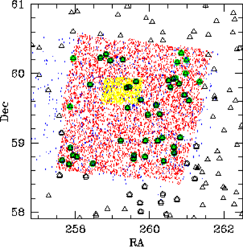
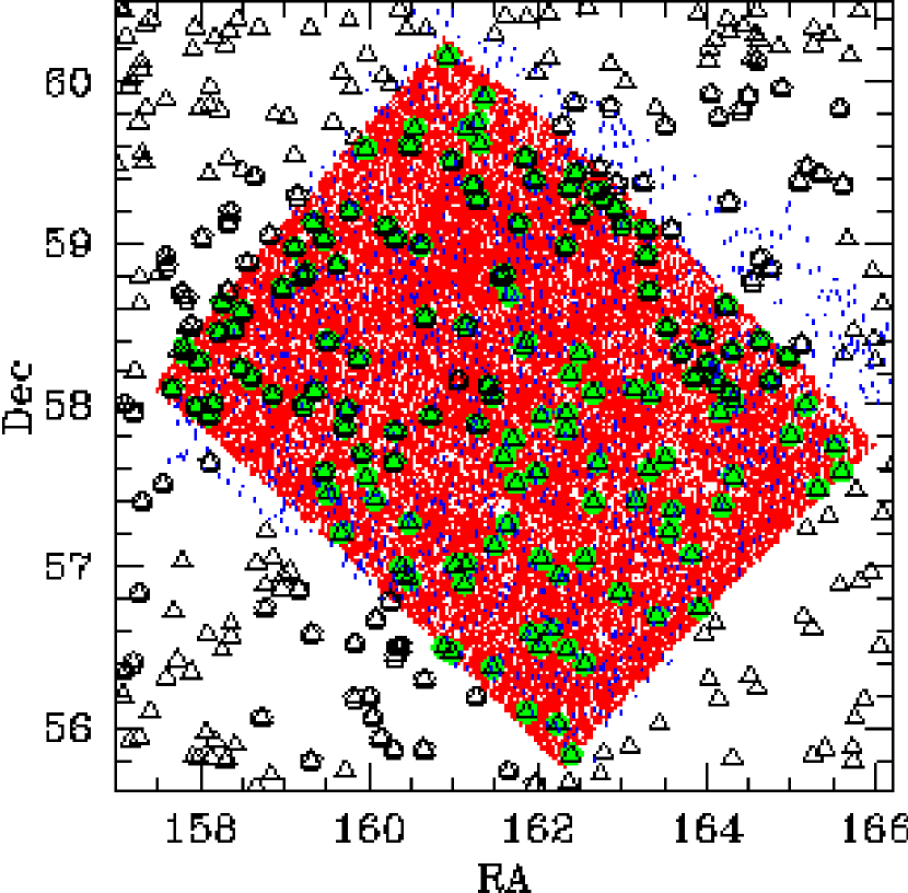
Figure 1: Location of SDSS-DR3 quasars in the XFLS (left) and SWIRE Lockman Hole (right) fields. Red/yellow/blue points are IRAC/IRACverification/MIPS70 sources. Open triangles are SDSS-DR3 quasars. Green circles are SDSS-DR3 quasars with IRAC detections in all 4 bands. Open pentagons indicate GALEX-detected SDSS quasars.

The 46,420 SDSS quasars of Schneider et al. (2005) are matched to IRAC detections in the XFLS (main_4band.cat; Lacy et al. 2005) and the SWIRE ELAIS-N1, -N2, and Lockman Hole (SWIRE2_N1_cat_IRAC24_16jun05.tbl, SWIRE2_N2_cat_IRAC24_16jun05.tbl, SWIRE2_Lockman_cat_IRAC24_10Nov05.tbl; Surace et al. 2005) areas of sky. The IRAC bandpasses are generally refereed to as Channels 1 through 4 or as the 3.6$\mu$m, 4.5$\mu$m, 5.8$\mu$m, and 8.0$\mu$m bands, respectively. For a quasar spectrum with $\alpha_{\nu}=-1$ ($f_{\nu}\propto\nu^{\alpha}$), the effective wavelengths of the IRAC bandpasses are actually closer to 3.52$\mu$m, 4.46$\mu$m, 5.67$\mu$m, and 7.70$\mu$m. The SWIRE catalogs also include $24\mu$m photometry from the Multiband Imaging Photometer for Spitzer (MIPS; Rieke et al. 2004). In the XFLS field, 24$\mu$m sources are cataloged by Fadda et al. (2006) and we include matches from that catalog as well. As the limits of the mid-IR catalogs are much deeper than the SDSS spectroscopic survey, we consider only objects detected in all 4 IRAC bands. Within a matching radius of $1\farcs 0$ there are 44 SDSS-DR3 quasar matches in the XFLS area, 29 in the ELAIS-N1 area, 44 in the ELAIS-N2 area, and 142 in the Lockman Hole area. All but one of the optically selected SDSS quasars has 4-band IRAC coverage in the regions of overlap between the SDSS and Spitzer data; see Figures 1 and  2. The exception being SDSSJ 104413.47+580858.9 ($z=3.7$) which has only a limit in IRAC channel 3.

To construct the most detailed quasar spectral energy distributions (SEDs) possible, we include data available at other wavelengths. We include matches to MIPS 70$\mu$m sources in the XFLS (FLS70_sn7_jul05.txt; Frayer et al. 2006) and in the SWIRE (SWIRE2_EN1_70um_23nov05.tbl, SWIRE2_EN2_70um_23nov05.tbl, SWIRE3_Lockman_70um_23nov05.tbl; Surace et al. 2005) areas. No MIPS 160$\mu$m data are included as the flux density limits of these data in the XFLS and SWIRE areas are much brighter than expected flux densities of even the brightest SDSS-DR3 quasars in these fields. For the SDSS quasars in the ELAIS fields we have extracted $15\mu m$ photometry from the Rowan-Robinson et al. (2004) catalog. We also extract $J/H/K$ and radio information from this catalog if that information was not otherwise available.

Some of these areas of sky have been observed by GALEX (Martin et al. 2005), and the data were released as part of GALEX-GR1. Quasars are readily detected by GALEX (see Bianchi et al. 2005 and Seibert et al. 2005), thus we also include GALEX photometry where available. Matching of the GALEX catalogs and the SDSS DR3 quasar sample is described by Trammell et al. (2005). The effective wavelengths of the GALEX NUV and FUV bandpasses (hereafter referred to as $n$ and $f$ magnitudes) are 1516Å and 2267Å. GALEX photometry has been corrected for Galactic extinction assuming $A_{n}/E(B-V)=8.741$ and $A_{f}/E(B-V)=8.376$ (Wyder et al. 2005). A total of 55 and 88 of the DR3 quasars have GALEX detections in the $f$- and $n$-bands, respectively.

In the radio, we have matched to the deeper VLA data taken in the XFLS area by Condon et al. (2003), which catalogs 5$\sigma$ detections with fluxes higher than 115$\mu$Jy (about an order of magnitude deeper than FIRST). Deep VLA data also exists for the ELAIS and Lockman Hole areas, but only over a small area of sky (e.g., Ciliegi et al. 1999, 2003).

Most of our objects are fainter than the 2MASS (Skrutskie et al. 1997) limits, but we have supplemental near-IR data for a few. Near-IR ($JHK_{s}$) magnitudes for SDSS J1716+5902 were obtained on UT 9 September 2003 using the GRIM II instrument on the Apache Point Observatory 3.5-m telescope. Dithered images were obtained and reduced in the standard fashion, using running flat-fielding and sky-subtraction (e.g., Hall, Green, & Cohen 1998) with all available good images in a given filter for each object. Four other sources (SDSSJ 171732.94+594747.5, SDSSJ 171736.90+593011.4, SDSSJ 171748.43+594820.6, and SDSSJ 171831.73+595309.4) were observed at Palomar Observatory.

Finally, to better characterize the optical+MIR color distribution of type 1 quasars, we include 87 broadline quasars that are fainter than the SDSS spectroscopic magnitude limit, but that were confirmed from Hectospec (Fabricant et al. 2005) follow-up of MIPS 24 $\mu$m sources by Papovich et al. (2005).

Tables Spectral Energy Distributions and Multiwavelength Selection of Type 1 Quasars and Spectral Energy Distributions and Multiwavelength Selection of Type 1 Quasars present all of the multiwavelength data for the SDSS-DR3 quasars in our sample. The columns in Table Spectral Energy Distributions and Multiwavelength Selection of Type 1 Quasars are name, redshift, bolometric luminosity (see § 6), integrated optical luminosity, integrated IR luminosity, bolometric correction (from rest-frame 5100Å to the bolometric luminosity), X-ray (ROSAT) count rate, GALEX $f$- and $n$-band magnitudes, SDSS $ugriz$ magnitudes. The columns in Table Spectral Energy Distributions and Multiwavelength Selection of Type 1 Quasars are name (again), $J/H/K$ magnitudes, Spitzer-IRAC 3.6, 4.5, 5.8, and 8.0$\mu$m flux densities, ISO 15$\mu$m flux density, Spitzer-MIPS 24 and 70$\mu$m flux densities, radio (VLA, 20 cm) flux density, and radio luminosity. Both Tables Spectral Energy Distributions and Multiwavelength Selection of Type 1 Quasars and Spectral Energy Distributions and Multiwavelength Selection of Type 1 Quasars report only the observed photometry of these sources; no host galaxy contamination has been removed (§ 5.2). Of these 259 quasars, 28 have ROSAT detections and 30 have radio detections. Of those 30 radio detections, only 8 are radio loud ($L_{\rm rad}>10^{33}$ erg s^-1 Hz^-1).

3 MIR/Optical Colors of Type 1 Quasars

Lacy et al. (2004a), Stern et al. (2005), and Hatziminaoglou et al. (2005) have already demonstrated that MIR selection of AGNs (both type 1 and type 2) from Spitzer photometry is very efficient. Here we demonstrate that this capability can be enhanced by including morphology and optical color information from SDSS. We concentrate on relatively unobscured type 1 quasars, but to the extent that dust-reddened type 1 quasars and obscured type 2 quasars are not extincted beyond the SDSS flux density limits, what we learn here will apply to those objects as well.

3.1 The Color-Redshift Relations

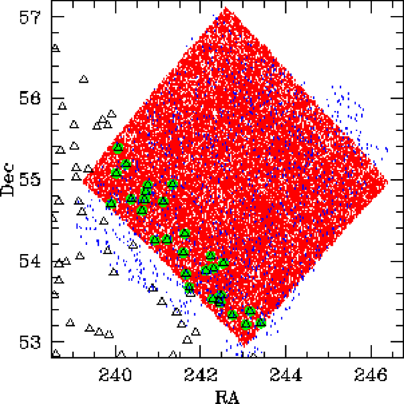
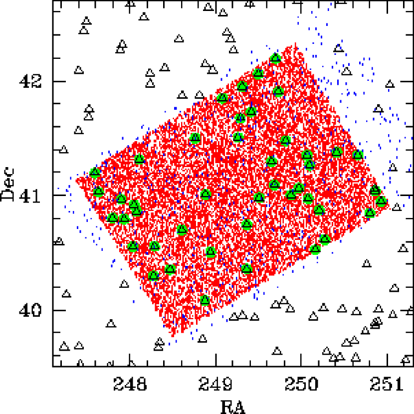
Figure 2: Location of SDSS-DR3 quasars in the SWIRE ELAIS N1 (left) and N2 (right) fields. Red points are 4-band IRAC sources. Blue points are MIPS 70 $\mu$m sources. Open triangles are SDSS-DR3 quasars. Green circles are SDSS-DR3 quasars with IRAC detections in all 4 bands.

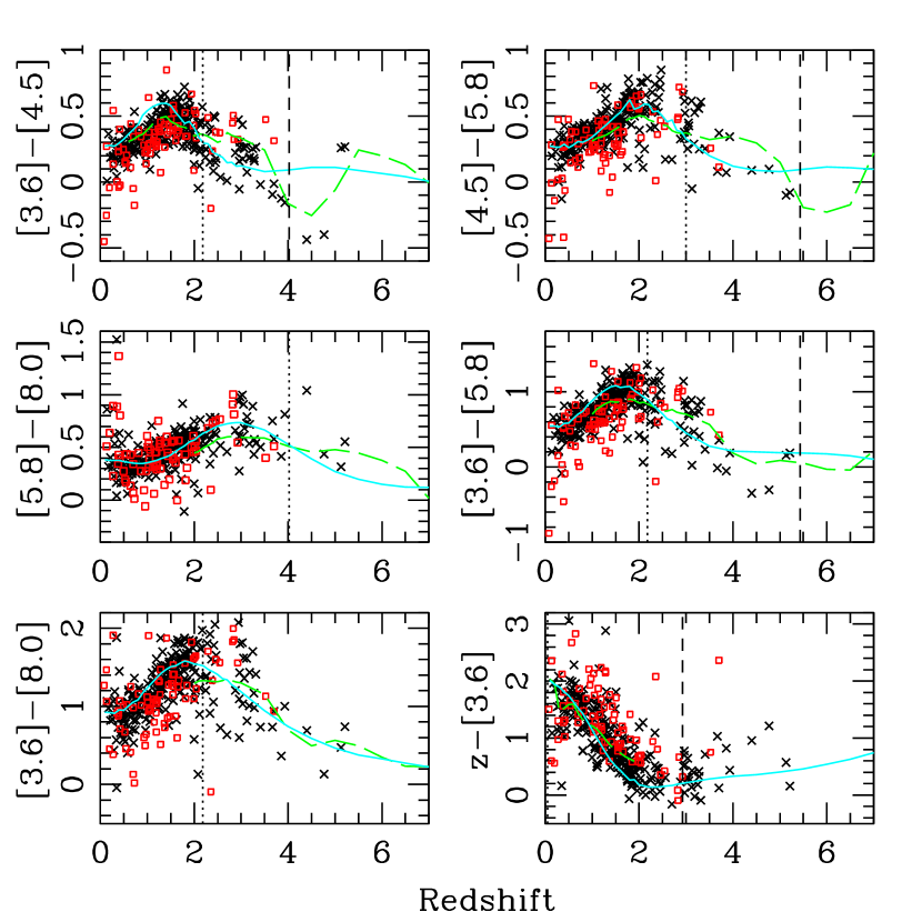
Figure 3: Color-redshift relation for various combinations of Spitzer colors. Black symbols are SDSS-DR3 quasars from the XFLS and SWIRE ELAIS-N1/N2 and Lockman Hole areas. Red points are Hectospec-confirmed XFLS quasars. Errors are typically $\sim 0.14$ mag. The dashed green curve is the expected relation found from convolving the geometric mean of the optical-IR composite spectrum of Glikman et al. (2005) with the transmission curves. The solid cyan curve is the expected relation from convolving the Elvis et al. (1994) composite radio-quiet SED with the transmission curves. The vertical lines mark the redshifts where 1$\mu$m enters the bluest (dotted) and leaves the reddest (dashed) band.

We begin by exploring the color-redshift relation for confirmed type 1 quasars. Figure 3 shows the color-redshift relation for various combinations of Spitzer colors; see Richards et al. (2003, Fig. 2) for similar plots using the SDSS bands. In Figure 3 black points are SDSS-DR3 quasars from the XFLS and SWIRE ELAIS-N1/N2 and Lockman Hole areas. Open red squares are Hectospec-confirmed XFLS quasars. The dashed green curve is the expected relation found from convolving the geometric mean of the optical-IR composite spectrum of Glikman et al. (2005) with the transmission curves. The solid cyan curve is the expected relation from convolving the Elvis et al. (1994) composite radio-quiet SED with the transmission curves. The Spitzer colors are given in AB magnitude units where $[1]-[2]=-2.5\log(S_{1}/S_{2})$.

Much of the color change seen in Figure 3 results from a single strong feature in the typical quasar SED — the so-called 1 micron inflexion, where the slope of the SED changes sign in a $\nu f_{\nu}$ vs. $\nu$ representation. Thus we have indicated (by dotted and dashed lines, respectively) where the $1\mu$m inflexion enters the bluest and leaves the reddest band. We extend the plot well beyond the redshifts of our confirmed quasars since Spitzer should be sensitive to quasars with redshifts in excess of $z=7$, and it is helpful to know the expected colors of such objects.

We show two sets of predicted color-redshift relations since, while the Elvis et al. (1994) template covers the the full redshift range, it is based in part on broad-band photometry, which smears out the effects of the emission lines. The spectroscopy-based curves derived from Glikman et al. (2005) will be more accurate in regions of strong emission lines, but this template covers a smaller wavelength (and thus redshift) range. For example the discrepancy at $z\sim 3$ and $z\sim 4.5$ in the $[3.6]-[4.5]$ color results from the H$\alpha$ line moving into and out of the filters. Colors derived from non-adjacent bandpasses show a much smaller effect as the emission lines are not simultaneously moving out of the bluer band and into the redder band. The smoothness of the color-redshift relations (as compared to the SDSS) and the relatively large ($\sim 10$%) photometric errors and means that IRAC colors alone may not be useful for accurate quasar photometric redshift estimation (e.g., Weinstein et al. 2004), but MIR color information in addition to optical colors will be extremely useful in breaking redshift degeneracies in the optical. Note in particular the very large change in $z-[3.6]$ color between redshifts 0 and 2 as the 1$\mu$m inflexion moves between those two bandpasses.

3.2 The Color-Color Relations

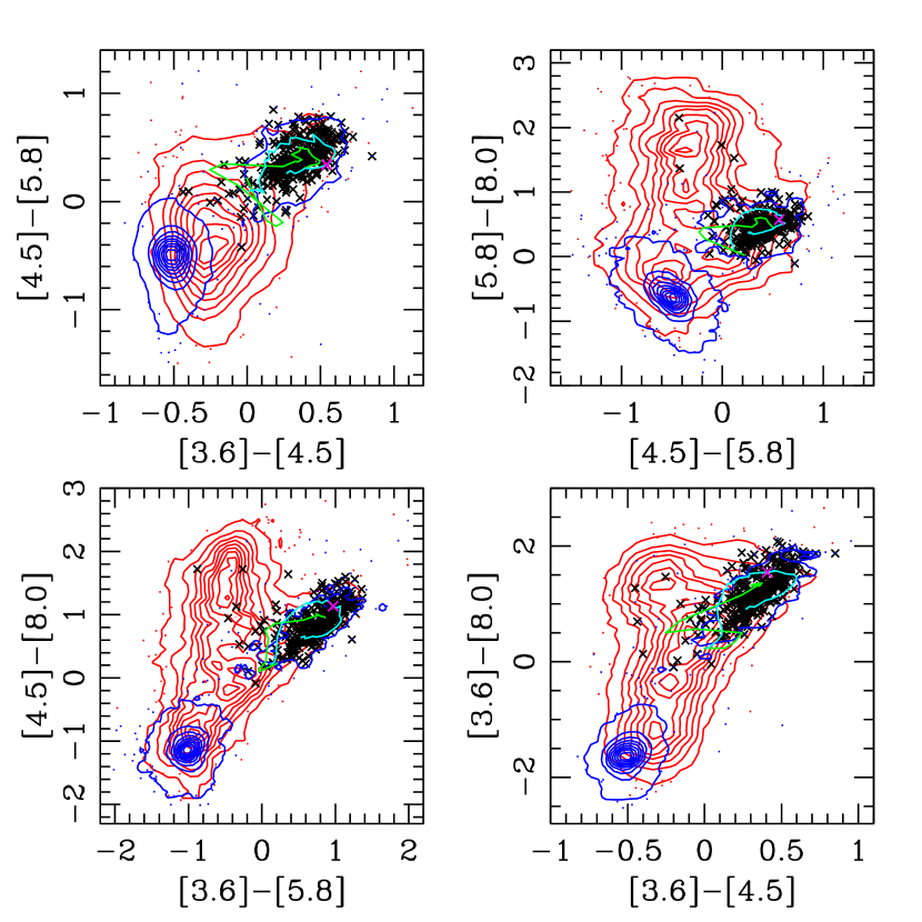
Figure 4: IRAC colors of SDSS+Spitzer objects. Blue contours and dots correspond to objects that have point-like SDSS morphologies, while objects classified by the SDSS as extended are shown by red contours and dots. These blue and red contours/dots represent all of the objects detected in all four IRAC bands in the XFLS catalogs that have a match in the SDSS-DR3 photometric database. Black symbols indicate spectroscopically confirmed type 1 quasars. The few outliers are from the Hectospec sample and may be mis-classified (or host galaxy dominated). The cyan lines are the $z=0.1$ to $z=7$ colors predicted from the Elvis et al. (1994) quasar SED; the highest redshift quasars are at the blue (negative) end of the tracks. The green line shows the predicted colors from $z=2$ ($z=1$ in the upper left-hand panel) to $z=7$ using the Glikman et al. (2005) composite spectrum. A magenta cross indicates where the lowest redshift from the Glikman et al. (2005) colors falls on the Elvis et al. (1994) curves. Redder colors have more positive values in this representation.

We next examine the distribution of type 1 quasars in color-color space. Lacy et al. (2004a), Stern et al. (2005), and Hatziminaoglou et al. (2005) have shown that AGN can be selected using only MIR colors such as those plotted in Figure 4. We plot all of the objects detected in all four IRAC bands in the XFLS catalog that have a match in the SDSS-DR3 photometric database. Blue contours and dots correspond to objects that have point-like SDSS morphologies, while objects classified by the SDSS as extended are shown by red contours and dots. Black symbols indicate the spectroscopically confirmed type 1 quasars. The cyan lines are the $z=0.1$ to $z=7$ colors predicted from the Elvis et al. (1994) quasar SED; the highest redshift quasars have the bluest (most negative) colors. The green lines show the predicted colors from the Glikman et al. (2005) composite spectrum from $z=2$ ($z=1$ in the upper left-hand panel, which does not depend on the 8$\mu$m band) to $z=7$. The magenta cross indicates the redshift along the Elvis et al. (1994) tracks where the Glikman et al. (2005) tracks start (either $z=2$ or $z=1$).

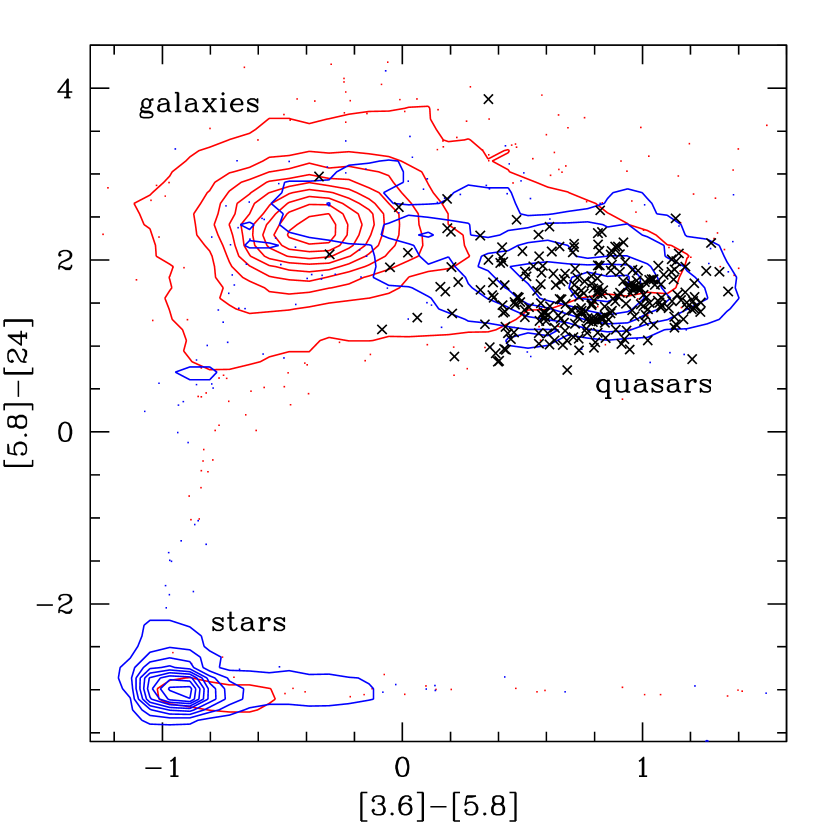
Figure 5: $[3.6]-[5.8]$ vs. $[5.8]-[24]$ colors of SDSS+Spitzer objects in the ELAIS areas. Contours and points are as in Fig. 4. Stars (which have very blue $[5.8]-[24]$ color and generally have point-like SDSS morphology classification) are much more cleanly separated from quasars and galaxies when the MIPS $24\mu$m data is included. However, little is gained in terms of galaxy-quasar separation as they have similarly red $[5.8]-[24]$ colors.

From these plots, especially $[3.6]-[5.8]$ vs. $[4.5]-[8.0]$ in the lower left-hand corner, it is clear that MIR colors combined with optical morphology can select type 1 quasars efficiently (and with a high degree of completeness) as point-like sources with red MIR colors. Luminous type 2 quasar candidates can also be identified as those extended sources with AGN-like IR colors. Adding the optical morphology information confirms the speculation of Lacy et al. (2004a) and Stern et al. (2005) regarding the nature of the two red branches, with point-like AGN dominating the objects with red $[3.6]-[5.8]$ color and extended sources (presumably low-redshift, PAH-dominated galaxies) populating the red $[4.5]-[8.0]$ branch. Adding this SDSS morphology information thus enhances the MIR color-classification of sources since the Spitzer PSF is too large to yield morphology information for distant sources. We further demonstrate the classification information that is gained by including morphology in Figure 5 where we add MIPS $24\mu$m data in order to show $[3.6]-[5.8]$ vs. $[5.8]-[24]$. Adding the longer wavelength MIPS information clearly helps to discriminate stars (which have very blue $[5.8]-[24]$ colors) from galaxies and quasars which have very red $[5.8]-[24]$ color); however, little is gained in terms of quasar-galaxy separation that was not already realized with the IRAC photometry.

While Hatziminaoglou et al. (2005) investigate both the MIR and optical colors of their sample, the combined optical+MIR colors are not considered for selection. This is appropriate given that the flux density limits of the Spitzer survey fields are much deeper than the spectroscopic limit of SDSS quasar survey (for a typical quasar SED) and the IR is much less affected by dust extinction (and thus is more representative of the quasar population at a given nuclear magnitude). However, the SDSS photometry goes more than 3 magnitudes deeper than most of the SDSS’s spectroscopic survey for quasars, and at $i=21$, quasars must be reddened by $E(B-V)\sim 0.57$ to be extincted out of the SDSS imaging in the $i$-band. As such, it is interesting to explore the selection of quasars using the combined SDSS plus Spitzer color information.

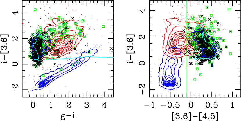
Figure 6: Color-color matrix using an SDSS color ($g-i$), an SDSS+Spitzer color ($i-[3.6]$), and a Spitzer color ($[3.6]-[4.5]$). See Fig. 4 for an explanation of the plot symbols. Combining Spitzer-IRAC photometry with SDSS colors/morphology defines a parameter space where stars, AGN, and normal galaxies can be efficiently distinguished. The green line in the right panel shows a possible selection criterion for unresolved AGN; open green squares show the point sources selected by such a cut. Black symbols are confirmed SDSS quasars. The cyan line shows the expected colors of quasars from $z=0.1$ to $z=5$ (using the Elvis et al. 1994 mean SED); low-redshift quasars having the reddest $i-[3.6]$ colors. The contours and dots are for XFLS sources only, whereas the black and green symbols are drawn from all four areas of sky in our sample.

Figure 6 shows the color-space distribution of our sources using an SDSS color, an SDSS+Spitzer color, and a Spitzer color. For the SDSS color, we choose $g-i$ since those are the most widely separated high S/N bands in the SDSS filter set. For SDSS+Spitzer, we chose the two closest high S/N bands ($i$ and $S_{3.6}$). For the Spitzer color, we chose the two highest S/N bands ($S_{3.6}$ and $S_{4.5}$); this choice happens to produce the greatest separation of classes and has the added attraction that it does not rely on the longer wavelength bands that will be lost when Spitzer’s coolant runs out. This presentation shows that AGN, normal galaxies, and stars can be separated quite cleanly when using both optical and near-IR information, particularly when morphology information is available in addition to the colors. If we were simply interested in selecting type 1 quasars, then selecting point sources with $[3.6]-[4.5]>-0.1$ might be sufficient given that such a cut includes nearly all of the point sources with non-stellar colors (with the exception of quasars near $z=4.5$, see Fig. 3). However, the morphology issue is complex. Including morphology means that normal galaxies will not contaminate the sample, but that type 2 AGN and faint AGN with poorly determined morphologies will be lost. Judicious rotation of the axes in Figure 6 may allow for relatively clean AGN selection without having to rely on morphology information. However, a better approach would be to take advantage of the 8-dimensional color space afforded by SDSS and Spitzer photometry and performing a Bayesian classification such as the kernel density estimation algorithm described by Richards et al. (2004). We intend to pursue such an approach in a future publication.

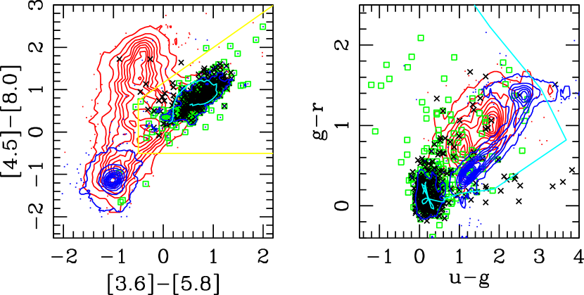
Figure 7: MIR (left) and optical (right) color-color plots showing the location of optical-color/morphology+MIR-color selected populations. See Fig. 4 for an explanation of the plot symbols. Quasar candidates (see Fig. 6) are shown as open green squares. The yellow lines in the left-hand panel show the MIR selection criteria from Lacy et al. (2004a) [after having multiplied their cuts by 2.5 to convert to a magnitude scale].

We can compare this optical+MIR selection to the MIR-only selection of Lacy et al. (2004a), Stern et al. (2005), and Hatziminaoglou et al. (2005). Each of these papers uses slightly different MIR selection techniques. We will compare explicitly only to Lacy et al. (2004a) as their selection is seen to empirically produce the greatest color separation with respect to morphology. In the left-hand panel of Figure 7 we reproduce the $[3.6]-[5.8]$ vs. $[4.5]-[8.0]$ color-color plot from Lacy et al. (2004a), showing their selection as yellow lines. Objects selected as being optical point sources with red MIR colors are shown as open green squares. Adding the optical data to the selection criteria allows us to select quasars more efficiently (with reduced completeness due to the loss of AGN dominated by host galaxy light in the optical). The right-hand panel of Figure 7 shows where these objects lie in $u-g$ vs. $g-r$ color space. For the sake of clarity, we have limited the point and extended sources to $g<21$ to reduce the scatter due to SDSS photometric error, but the green squares (point-like quasar candidates) have no such limit applied. We note that, despite the MIR color selection, the green squares are still predominantly UV-excess sources. To $i<21$, we find that 70% of the MIR color-selected quasars have $u-g<0.6$ and $g-r<0.6$. Thus, the fraction of dust-reddened/extincted type 1 quasars (e.g., Richards et al. 2003; Glikman et al. 2004) that might be missed by an optical survey with UVX color-selection is no larger than 30%. This limit applies to quasars with $i$-band extinction less than 1.0 mag (the difference between the SDSS $i$-band imaging limit and our adopted cut of $i=21$), which is $E(B-V)=0.48$ for Galactic extinction. This fraction may be higher if there are type 1 quasars with larger extinction, but is most likely smaller than 30% since many of the non-UVX quasars will simply have $z\gtrsim 2.2$. Quasars with $z>2.2$ have redder optical colors even if they are not dust-reddened; this population will still be identified by the SDSS quasar-selection algorithm.

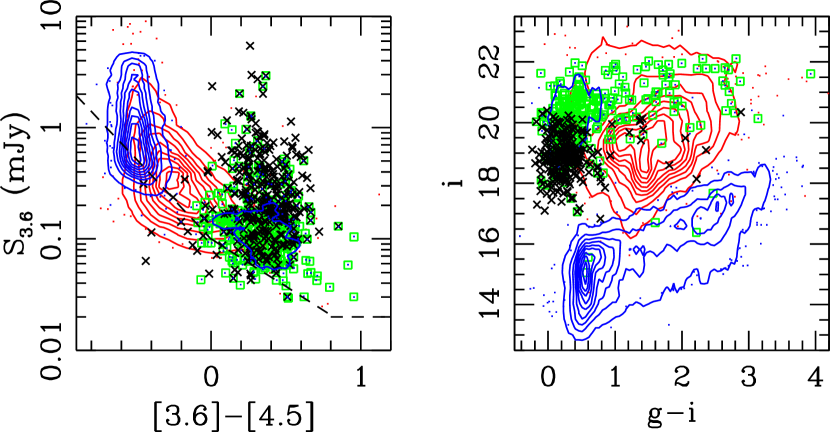
Figure 8: Left: Spitzer color-magnitude diagram. The dashed lines show the effects of the 5.8$\mu$m and 8.0$\mu$m flux density limits. Right: SDSS color-magnitude diagram. Faint ($i\gtrsim 18$) point sources with $g-i\gtrsim 0.8$ are either high-redshift quasars or dust-reddened low-redshift quasars. In both panels, the contours/points are coded the same as in Fig. 6.

Figure 8 shows color-magnitude plots for this selection criterion as compared with known quasars and point/extended sources in general. The 3.6$\mu$m flux density is limited for $[3.6]-[4.5]<0.0$ by the 8.0$\mu$m flux density limit and for $0.0<[3.6]-[4.5]<0.8$ by the 5.8$\mu$m flux density limit, as shown by the dashed lines. Note that while the 3.6$\mu$m flux density limit is 20$\mu$Jy, a 3.6$\mu$m selected sample is complete to all AGNs to only $\sim 200\mu$Jy. In the right-hand panel we again see that the density of dust-reddened and extincted type 1 quasars cannot be too large since the density of quasars with $i<19$ and $g-i<0.8$ is much higher than that of $i<22$ quasar candidates with $g-i>0.8$. This figure also serves to illustrate that MIR-only selection is most efficient for bright MIR sources. For $S_{3.6}>1$mJy there is little contamination of the MIR color space of AGNs, but at fainter limits, contamination from star-forming galaxies becomes problematic without additional selection information (such as the optical morphology).

4 The Obscured Quasar Fraction

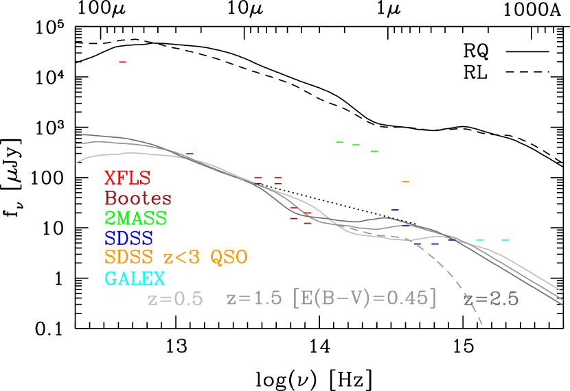
Figure 9: Mean quasar SEDs compared to various survey flux limits. The black solid and dashed lines are the $z=0$ Elvis et al. (1994) mean radio-quiet and radio-loud SEDs, normalized to $i=16.4$ (1 mJy). The colored dashes show the flux density limits for the Spitzer-XFLS, Spitzer-Boötes (Stern et al. 2005), 2MASS, SDSS (imaging), SDSS (low-z quasar spectroscopy) and GALEX. The lighter gray lines show the radio-quiet SED at $z=0.5$, $1.5$, and $2.5$ normalized to the Boötes field $8\mu$m flux limit (dashed gray line is $z=1.5$ reddened by $E(B-V)=0.25$). The dotted line shows a spectral index of $\alpha_{\nu}=-0.73$ between $8\mu$m and the SDSS $r$ band.

Here we make some comparisons between mid-IR only selection and optical+mid-IR selection in terms of relative flux limits. Figure 9 shows mean quasar SEDs compared to various survey flux limits. The black solid and dashed lines are the (rest-frame) Elvis et al. (1994) mean radio-quiet and radio-loud SEDs, normalized to $i=16.4$ (1 mJy). The colored dashes show the flux density limits for the Spitzer-XFLS, Spitzer-NOAO/Boötes (Jannuzi & Dey 1999; Eisenhardt et al. 2004), 2MASS, SDSS (imaging), SDSS ($z<3$ quasar spectroscopy), and GALEX. The lighter gray lines show the radio-quiet SED at z=$0.5$, $1.5$, and $2.5$ normalized to the Boötes field $8\mu$m flux limit. The dashed gray line shows the $z=1.5$ SED reddened by SMC-like reddening with $E(B-V)=0.45$. The Spitzer flux density limits of the Boötes and FLS areas are shown as brown and red bars. The 2MASS limits are given in green. The SDSS imaging limits are shown in blue, with the spectroscopic limit shown in orange. Cyan bars show the GALEX flux density limits (for the Medium Imaging Survey [MIS]).

Stern et al. (2005) estimate the fraction of obscured quasars missed by optical surveys by comparing their $8\mu$m source counts to the source counts of quasars at $R\sim 21$, assuming a spectral index of $\alpha_{\nu}=-0.73$. We revisit this analysis with two new considerations. First, we use the number counts of optically selected ($g$-band) quasars from Richards et al. (2005) which used SDSS imaging coupled with 2dF spectroscopy to determine the quasar luminosity function to $g\sim 21.5$. Second, rather than assuming a power-law SED, we use an empirical SED such as that from Elvis et al. (1994).

Stern et al. (2005) reported an obscured quasar fraction of $(275-65)/275=76$%, where 275 is their candidate AGN density per square degree and 65 is the density of optically selected AGN to $R=21$ from Wolf et al. (2003). We find that a typical quasar with an 8$\mu$m flux density of 76$\mu$Jy has a $g$-band magnitude of 21.5. Using the quasar luminosity function of Richards et al. (2005), we find an optically selected quasar density of 89 per square degree to $g=21.5$. This density gives an upper limit to the obscured fraction of $(275-89)/275=68$%.

However, since the quasar SED is not a power law between the optical and MIR, but rather exhibits some significant features (such as the 1$\mu$m inflexion), it is important to determine the $g$-band flux limit as a function of redshift. The expected flux density of a type 1 quasar with an 8$\mu$m flux density of 76$\mu$Jy can reach as faint as $g=22.5$ depending on redshift (and thus the optical counts will be underestimated). At that magnitude limit there are 170 optically selected quasars per square degree. We illustrate this issue in Figure 9 where one can see that at $z=0.5$ the expected $g$ and $r$ flux densities of a typical quasar are much fainter (but still detectable by SDSS) than the optical-to-MIR flux ratio assumed by Stern et al. (2005) (dotted line). While the density of luminous quasars peaks at $z\sim 2.5$ where the Stern et al. (2005) extrapolation is roughly correct, X-ray surveys (e.g., Ueda et al. 2003) have shown that the density of lower luminosity AGNs peaks at lower redshifts and thus this effect is important.

If we instead use our the mean SED that we will derive in § 5.2, the $g$-band magnitude for a 76$\mu$Jy source at $8\mu$m ranges between $g=21.4$ and $g=22.4$. The optically selected quasar densities for those magnitudes are 82 and 161 per square degree, respectively. Using these numbers, we find that the fraction of obscured quasars has a lower limit in the ballpark of $(275-161)/275=41$%. Finally, since the Stern et al. (2005) MIR-selected AGNs were selected to a rather faint MIR flux limit, then, as discussed above, some fraction of the AGN candidates may instead turn out to be normal star forming galaxies, which would also reduced the obscured quasar fraction.

Similar arguments can be made with regard to the obscured quasar fraction computed by Lacy et al. (2004a). They found an obscured fraction of $(16/35)=46$% by assuming that all 8$\mu$m sources brighter than 1 mJy would be brighter than the SDSS’s spectroscopic magnitude limit of $i=19.1$. Using the Elvis et al. (1994) SED to determine the $i$ magnitude for this 8$\mu$m flux density as a function of redshift, we find that many IR-bright, low redshift quasars will in fact be fainter than the SDSS spectroscopic limit. Again, this effect is largest at low redshift, but Lacy et al. (2004a) find their obscured-AGN candidates are primarily low redshift. In principle, this would suggest that the obscured quasar fraction found by Lacy et al. (2004a) is also an upper limit; however, in practice, their objects do appear to be bona-fide obscured AGNs (Lacy et al. 2004b). This may be due in part to the much brighter MIR flux limit imposed by Lacy et al. (2004a) (as compared to Stern et al. 2005). Nevertheless, we caution that the shape of the SED can influence the expected MIR-to-optical ratio of quasars as a function of redshift.

Other work on obscured AGN using Spitzer selection has typically suggested a large obscured quasar fraction. Martínez-Sansigre et al. (2005) use a combined radio and Spitzer 24$\mu$m based selection in the XFLS to show that the ratio of obscured to type-1 quasars is in the range 1–$3:1$, but this estimate is dependent on a lack of evolution in the distribution of the ratio of radio to optical luminosities of quasars from low to high redshifts, as the majority of high redshift quasars are expected to have much lower radio luminosities than probed by the radio survey of the XFLS by Condon et al. (2003). The deep, multi-wavelength Great Observatories Origins Deep Survey (GOODS) finds a ratio of obscured to unobscured AGN of $\sim 3:1$ (Treister et al. 2004), but most of their AGN are well below quasar luminosity, and thus not directly comparable to the objects studied in this paper. It is also important to realize that mid-infrared selection may not find all obscured quasars, particularly at high redshift, where the IRAC bands are redshifted into the rest-frame near infrared, or in cases of objects viewed through very high ($A_{V}\sim 100$) extinctions, as expected for objects viewed through an obscuring torus edge-on to the line of sight. Improved modeling of the biases in mid-infrared selection of AGN should remove much of this uncertainty.

5 Spectral Energy Distributions

5.1 Introduction

Accurate determination of quasar SEDs is crucial to our understanding of quasar physics. The strengths and shapes of the various components of a typical quasar SED have been used to determine the physical drivers in each frequency regime from the jets in the radio to the dusty torus in the mid-to far-IR, the accretion disk in the optical/UV/soft-X-ray, and the X-ray corona at the highest energies.

As the observed radiation from quasars is often re-processed and re-emitted at wavelengths far different from the seed photons, knowing the overall SED is necessary for determining bolometric luminosities. In turn, bolometric luminosities are necessary for determining the so-called Eddington ratio ($L_{\rm bol}/L_{\rm Edd}$, or equivalently $L_{\rm bol}/M_{\rm BH}$), which serves as a measure of the accretion rate of the system (e.g., Peterson 1997).

Despite a few recent additions/updates to Elvis et al. (1994), (e.g., Polletta et al. 2000; Kuraszkiewicz et al. 2003; Risaliti & Elvis 2004), complete SEDs have been compiled for only a small number ($\lesssim 100$) of quasars and the mean SED from Elvis et al. (1994) is arguably still the best description of the SED of quasars and is certainly the most commonly used. However, it is illuminating to recall the caveats given by the authors in the abstract of that paper: “We derive the mean energy distribution (MED) for radio-loud and radio-quiet objects and present the bolometric corrections derived from it. We note, however, that the dispersion about this mean is large ($\sim 1$ decade for both the infrared and ultraviolet components when the MED is normalized at the near-infrared inflection). … The existence of such a large dispersion indicates that the MED reflects on some of the properties of quasars and so should be used only with caution.”

Furthermore, in addition to the SED diversity in their sample, it is well known that the sample used to construct this mean SED is not entirely representative: “Our primary selection criteria were (1) existing Einstein observations at good signal-to-noise ratio (to ensure good X-ray spectra) and (2) an optical magnitude bright enough to make an IUE spectrum obtainable.” The first criterion means that the sample is biased toward towards X-ray bright quasars, and therefore typically objects with relatively high X-ray-to-optical flux ratios. Similarly, the second criterion biases the sample towards bluer quasars (see Jester et al. 2005).

Nevertheless, the mean SED from Elvis et al. (1994) has generally been found to be a robust template for typical type 1 quasars. However, given the diversity of the mean SED, the biases inherent to the sample, and the accuracy to which we would like to know the bolometric luminosity for a given quasar, it is important to improve our knowledge of the full SED of quasars to test how well this assumption holds and to investigate the full range of individual SEDs.

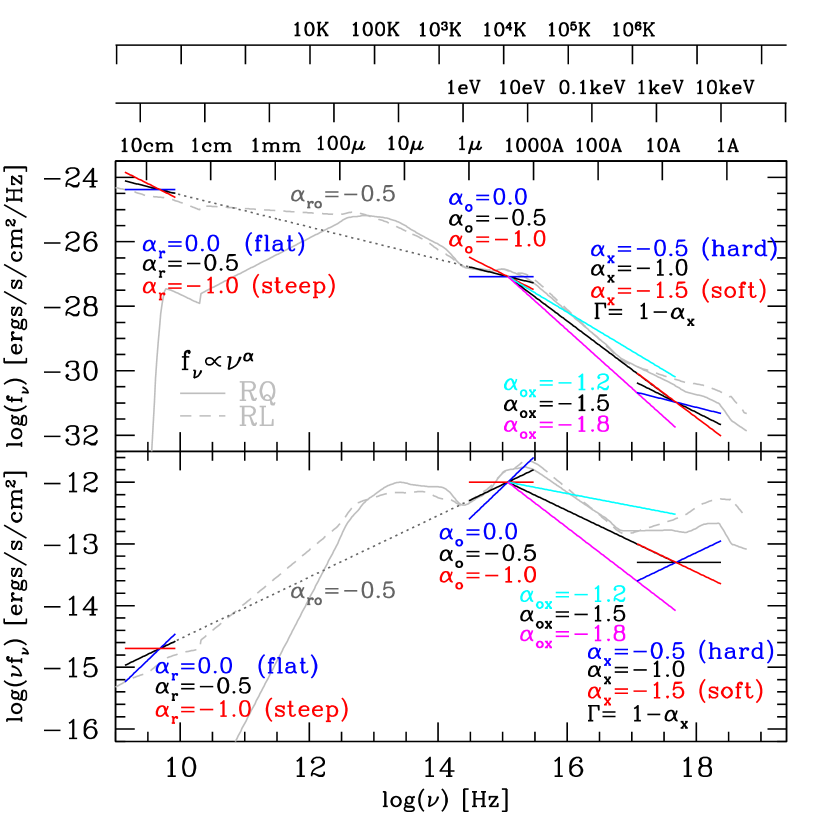
Figure 10: Quasar SED diagnostic plot. Show in gray are the Elvis et al. (1994) radio-quiet (solid) and radio-loud (dashed) mean SEDs. The colored lines indicate typical spectral indices in the radio, optical, and X-ray using the same sign convention. Also shown is the typical radio-to-optical spectral index for radio-loud quasars and the range of optical-to-X-ray spectral indices. Studies in different bands tend to use different sign conventions for spectral indices and jargon to describe them (e.g., steep/red/soft). The top panel shows $f_{\nu}$, while the bottom panel shows $\nu f_{\nu}$. The $x$-axis is labeled as log($\nu$) (bottom), and wavelength, energy, and temperature (top).

As there is often little overlap in the jargon and notation used to describe quasars in different bandpasses (e.g. blue/red/Angstroms/magnitudes in the optical, flat/steep/GHz/mJy in the radio, hard/soft/keV/cgs in the X-ray), it will aid our discussion to review quasar SEDs from a single multi-wavelength point of view. Thus in Figure 10 we show the mean radio-loud and radio-quiet quasar SEDs from Elvis et al. (1994) on a log-log plot of $f_{\nu}$ vs. ${\nu}$ (top panel) and $\nu f_{\nu}$ vs. ${\nu}$ (bottom panel). Here $f_{\nu}$ is given in ergs s^-1 cm^-2 Hz^-1, and the abscissa is given in log frequency, wavelength, energy, and temperature units. The normalization is such that the quasar has a continuum flux density of 0.08 mJy ($AB=19.1$) at 2500Å. Typical ranges of spectral indices within and between bands are shown; the spectral indices are given as energy indices where $f_{\nu}\propto\nu^{\alpha}$ such that $\alpha$ represents the slope (and is thus generally negative).

We wish to use Figure 10 to make a few points. First, there is considerable scatter in quasar SEDs in each energy regime and little is known about correlations in these variations between energy regimes. Second, the plots visually emphasize the point made above, which is that the Elvis et al. (1994) sample was quite X-ray bright. Finally, there is a strong need for better characterization of quasar SEDs in the near- through far-IR.

5.2 Mean SEDs

To explore the color and luminosity dependence of the quasar SED, we use the 259 SDSS quasars cataloged herein to construct new mean SEDs. The individual SEDs of these quasars are shown in the Appendix. For the sake of homogeneity, we have excluded the Hectospec-confirmed quasars from Papovich et al. (2005) as they were selected with different criteria than the SDSS-confirmed quasars.

These SEDs are constructed as follows. While all of our objects have 5 SDSS magnitudes and 4 Spitzer-IRAC flux densities, many objects have no measurements in the 10 other bands that we catalog. Thus we first attempt a form of “gap-repair”. For the GALEX $f$- and $n$-bands, $J$, $H$, and $K$, the ISO 15$\mu$m-band, and the Spitzer-MIPS 24 and 70$\mu$m bands, we replace missing values with those determined from normalizing the Elvis et al. (1994) SED in the next nearest bandpass for which we have data. For example, $n$ is estimated from $u$, $J$ from $z$, $K$ from $S_{3.6}$, $S_{15}$ from $S_{8.0}$, etc. For the radio-loud quasars we use the Elvis et al. (1994) mean radio-loud SED; the remaining quasars are repaired using the Elvis et al. (1994) mean radio-quiet SED.

Since the optical-to-X-ray flux ratio of the Elvis et al. (1994) SED is somewhat abnormal, we do not perform the same sort of gap repair in the X-ray for those quasars that lack ROSAT detections. Instead, we use the $L_{UV}$–$L_{X}$ relationship that has been known since Avni & Tananbaum (1986) and has been well-characterized by Strateva et al. (2005). This relationship parameterizes the relatively tight correlation between the 2500Å and 2 keV brightness of quasars as a function of luminosity. Thus we normalize the Elvis et al. (1994) SED to the average of the high S/N ($gri$) SDSS measurements and determine the 2500Å flux density for that normalization. Then we use the equations given by Strateva et al. (2005) to estimate the 2 keV flux density of each quasars. We then assume a flat (in $\nu f_{\nu}$ space, which has $\alpha_{x}=-1.0$) spectrum between 0.1 and 10 keV, roughly consistent with Reeves & Turner (2000) and George et al. (2000). Finally, as there are only 8 radio-loud quasars in our sample and wavelengths shortward of $\sim 100\mu$m are energetically unimportant, we ignore any missing radio information (though all the objects have upper limits).

In addition to gap-repair, it is necessary to correct for host galaxy contamination, which can have a significant effect in many of the bandpasses that we consider. Lacking the data to measure the host galaxies of our sources, we must estimate their contribution. Such estimates of the contribution of host galaxy light to the SEDs can be made by applying simple scaling relationships among host bulge luminosity, bulge mass, black hole mass, and Eddington luminosity (e.g., Dunlop et al. 2003; Vanden Berk et al. 2006). The well-known correlation between central black hole mass and both bulge mass and luminosity (e.g., Ferrarese 2002) implies that quasars accreting at near their Eddington limits must have host bulge masses, and therefore luminosities, large enough to harbor the inferred black hole. We have used the quasar luminosity vs. host luminosity relationship at optical frequencies, described by Vanden Berk et al. (2006), to estimate the relative host galaxy contribution, assuming that the quasars are emitting at their Eddington limits.

We specifically convert the $M_{r}$ relationship used by Vanden Berk et al. (2006) to a luminosity and determine the host galaxy luminosity as

$$\log(L_{\rm Host})=0.87\log(L_{\rm AGN})+2.887-\log(L_{\rm Bol}/L_{\rm Edd}),$$ (1)

where the host galaxy and AGN luminosities are specific luminosities at 6156Å (the effective wavelength of the SDSS $r$ band) and we have taken $L_{\rm Bol}/L_{\rm Edd}$ to be unity. This synthesis of multiple scaling relations will have considerable scatter, and many, if not most, AGNs will be accreting at much lower Eddington ratios. However, we have found that a value of $(L_{\rm Bol}/L_{\rm Edd})=1$ works well and it has the nice feature that it represents the minimum host galaxy contribution that must be accounted for (smaller ratios implying relatively more luminous hosts).

This process sets the relative scaling of the host galaxy in the optical bandpasses. To actually subtract the host galaxy contribution at all wavelengths, we use the elliptical galaxy template of Fioc & Rocca-Volmerange (1997) scaled according to the prescription above. We ignore the differences between spiral and elliptical hosts as the host galaxy contribution is small where these differences matter most. Using this template and the above scaling, we find that at its peak ($\sim 1.6\mu$m), the host galaxy contributes between 30 and 38% of the total observed luminosity. This fraction approaches unity for $(L_{\rm Bol}/L_{\rm Edd})=1/3$. In practice, we have removed the host galaxy contribution before applying the above gap-repair process since the Elvis et al. (1994) template has already been corrected for the host galaxy contribution.

As we wish to investigate the mean properties of quasars as a function of luminosity, color, etc., we next combine the corrected individual SEDs and construct a number of different mean SEDs. We first convert the flux densities of each individual object to luminosities in our adopted cosmology and shift the bandpasses to the rest-frame. We then create a grid of points separated by 0.02 in log frequency and linearly interpolate between the 19 rest-frame effective frequencies that are populated by our gap-repaired photometry.

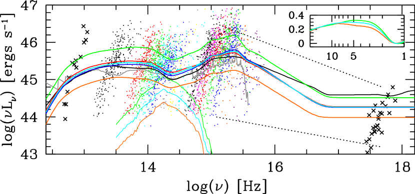
Figure 11: Mean quasar SEDs and the data used to construct them. The points show the data; the lines show the mean SEDs. From left to right: black crosses–MIPS70, black points–MIPS24/ISO15, red points–$S_{8.0}$, green points–$S_{5.8}$, cyan points–$S_{4.5}$, blue points–$S_{3.6}$, gray points–$K$, yellow points–$H$, cyan points–$J$, black points–$z$, magenta points–$i$, red points–$r$, green points–$g$, blue points–$u$, orange points–$n$, purple points–$f$, black crosses–x-ray. The dotted lines show the range of $\alpha_{\rm ox}$ with luminosity for the luminosity extremes of our sample (Strateva et al. 2005). From top to bottom (at $10^{14}$ Hz) the thick solid lines are green–optically luminous SDSS quasars, red–optically red SDSS quasars, cyan–all SDSS quasars, blue–optically blue SDSS quasars, black–Elvis et al. (1994) radio-quiet mean SED, gray–Hatziminaoglou et al. (2005) mean SED (normalized to Elvis et al. 1994 at $1\mu$m), orange–optically dim SDSS quasars. The near-IR luminous/dim composites are nearly identical to the optical composites. The thin green, cyan and orange curves show the host galaxy contribution assuming $(L_{\rm Bol}/L_{\rm Edd})=1$ (see Eq. 1) for the elliptical galaxy composite spectrum of Fioc & Rocca-Volmerange (1997). The dashed cyan curve shows the effect of ignoring the host contribution. The inset at the upper right zooms in on the MIR region of the spectrum. The three curves are normalized at 1.3$\mu$m and the $y$-axis shows relative luminosity, while the $x$-axis is in microns.

The resulting mean SEDs are shown in Figure 11, where the mean radio-quiet SED from Elvis et al. (1994) is shown in black and the mean SED from Hatziminaoglou et al. (2005) is shown in gray (normalized to the black curve at $1\mu$m). The individual data points for our quasars are also shown, color-coded by band. The mean of all our objects is shown in cyan. We have further constructed mean SEDs for the optically luminous/dim and optically blue/red halves of the population as shown in green, orange, blue, and red, respectively. The median values used to split the distributions are optical: $\log(L)=46.02$; IR: $\log(L)=46.04$; color: $\Delta(g-i)=-0.04$; where extremely red quasars having $\Delta(g-i)>0.3$ were excluded from the construction of all the composite SEDs (19 quasars in all). These mean SEDs are given in tabular form in Table Spectral Energy Distributions and Multiwavelength Selection of Type 1 Quasars. The thin lines show the relative host galaxy contribution for the luminous (green), all (cyan), and dim (orange) samples using the scaling and galaxy template as described above. The dashed cyan line shows the effect of ignoring the host contribution for the full-sample mean SED.

One of the primary purposes of constructing these mean SEDs as a function of various quasar properties is to see how the MIR part of the SED changes with these properties. Interestingly, we find that the shape of the MIR part of the SED is very similar for optically blue and optically red quasars. However, there are significant differences between the most- and least-optically luminous quasars in our sample. The inset of Figure 11 shows that the luminous quasars are much brighter in the 4$\mu$m region than the least luminous quasars. These differences have the potential for being diagnostics for the physical parameters (such as orientation and dust temperature) that go into AGN dust models (e.g., Nenkova, Ivezić, & Elitzur 2002; Dullemond & van Bemmel 2005). Spitzer-IRS spectra are needed to determine if these are truly broad features or if perhaps they are due to emission lines (e.g., Pa$\alpha$ and Br$\alpha$, which are at 4.05$\mu$m and 1.88$\mu$m, respectively). In the next section, we will investigate the differences between these SEDs in terms of the bolometric corrections derived from them.

6 Bolometric Luminosities and Accretion Rates

The determinations of quasar physical parameters such as bolometric luminosity, black hole mass, and accretion rate have been revolutionized by two bodies of work from the past decade. The first is the construction of mean quasars SED such as by Elvis et al. (1994), which allows one to estimate the bolometric luminosity of a quasar from a monochromatic luminosity and the assumption of a standard SED. The other is the reverberation mapping work led by Wandel, Peterson, & Malkan (1999) and Kaspi et al. (2000) (see also Kaspi et al. 2005) which allows one to infer a characteristic radius for the broad emission line region from the bolometric luminosity of the object and thus to relate the widths of emission lines to the mass of the central black hole. With these two pieces of information, we can derive a third (related) quasar property — the Eddington ratio ($L_{\rm Bol}/L_{\rm Edd}$, or equivalently $L_{\rm bol}/M_{\rm BH}$), which is a measure of the accretion rate.

Our primary purpose for constructing these new SEDs is to investigate how the bolometric luminosities and accretion rates derived from them differ from those determined by assuming the mean SED from Elvis et al. (1994). As discussed above, the biases inherent to the sample of objects used by Elvis et al. (1994) in addition to the warnings by Elvis et al. (1994) of the diversity of individual SEDs, coupled with the use of their mean SED as a single universal template, is what motivates this investigation.

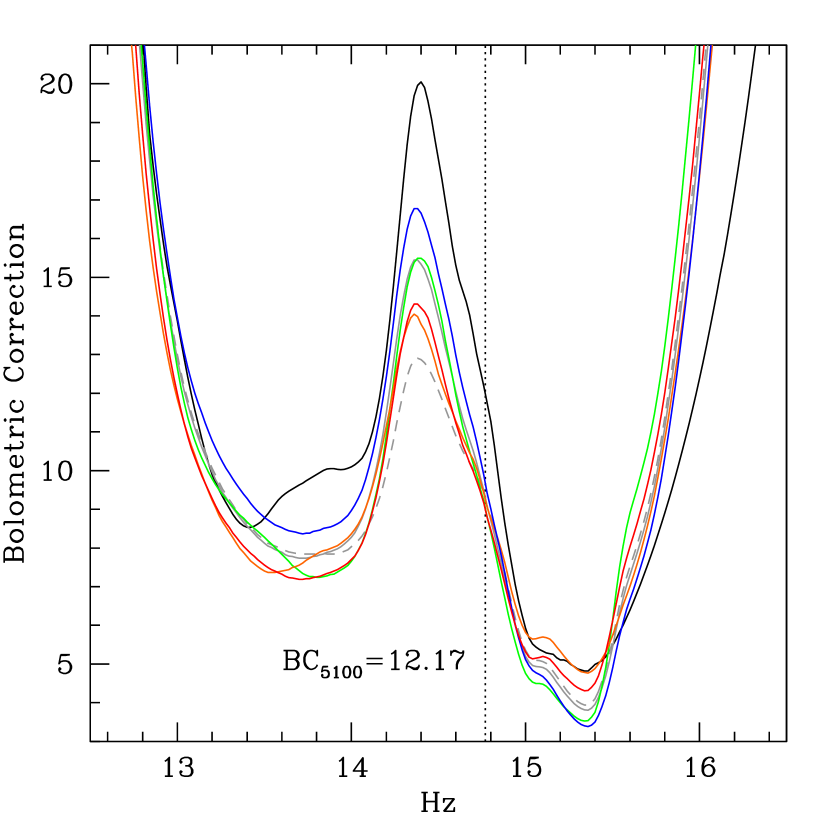
Figure 12: Bolometric corrections as a function of frequency for the SEDs in Fig. 11, the color coding is the same as for the previous figure (except that the full SDSS-DR3 mean quasar SED is now shown in gray instead of cyan). The dashed gray curve shows the full-sample mean SED without correction for the host galaxy contribution. The bolometric correction from 5100Å for the Elvis et al. (1994) radio-quiet SED is 12.17 (dotted line).

Figure 12 shows the frequency-dependent bolometric corrections (where the bolometric luminosity is taken to be the 100$\mu$m to 10 keV integrated luminosity) derived from each of the mean SEDs shown in Figure 11. The bolometric correction from 5100Å for the Elvis et al. (1994) radio-quiet SED is 12.17. The scale in Figure 12 (compared to that in Fig. 11) further highlights the differences between the mean SED shapes. As our SDSS-selected sample is less biased than that of Elvis et al. (1994), it should provide a more robust template for type 1 quasars, and further, the larger sample of objects allows us to consider the quasar SED not only in the mean, but as a function of various quasar properties. We see that in the MIR in particular, it is important to consider the range of SEDs possible when converting a monochromatic MIR luminosity to a bolometric luminosity. Curiously, in the rest-frame optical, where bolometric corrections are normally determined (usually at 5100Å), the differences in the composite SEDs are quite minimal. It may be that this lack of a difference results from this region being a relative minimum in the combination of host galaxy contamination in the near-IR and dust extinction in the UV.

Looking at the mean SEDs underscores the differences for individual objects, however. Figure 13 shows a histogram of the individual bolometric corrections for each quasar in our sample. These values (and $L_{\rm bol}$) are also given in Table Spectral Energy Distributions and Multiwavelength Selection of Type 1 Quasars. The mean B-band bolometric correction from Elvis et al. (1994) was 11.8 with a range of [5.5,24.7]; our mean and standard deviation are $10.4\pm 2.5$. In this figure, we see that the average quasar has its bolometric luminosity overestimated by $\sim$17% when using the Elvis et al. (1994) SED and that objects can have their bolometric luminosities mis-estimated by up to a factor of 2. These errors propagate directly to errors in the accretion rate. Unfortunately, we find no strong trends between the bolometric correction and color or luminosity. Thus it is difficult to know when to apply anything other than the mean bolometric correction. Clearly, if we are ever to understand the accretion rate distribution of quasars, we must attempt to determine bolometric corrections to an accuracy better than that which is afforded by assuming the mean SED.

A final caveat is that it must be understood that bolometric corrections and bolometric luminosities determined by summing up all of the observed flux are really line-of-sight values that assume that quasars emit isotropically, when, in fact, we know that this is not the case. For example, the same quasar seen both face-on and edge-on need not yield SEDs that sum to the same bolometric luminosity; all of the energy must eventually escape, but not necessarily equally along all lines of sight. Thus in Table Spectral Energy Distributions and Multiwavelength Selection of Type 1 Quasars, in addition to the bolometric luminosity, we also compute the integrated optical and IR luminosities. The integrated IR luminosity may be a more appropriate luminosity measure if the IR emission is largely isotropic (although even at $30\mu$m, IR emission is expected to be highly anisotropic; van Bemmel & Dullemond 2003). Alternatively, one might prefer to use the integrated optical/UV luminosity since nearly all photons emitted at other wavelengths by AGNs are reprocessed optical/UV/soft-X-ray seed photons. In either case, until we fully understand the SEDs of quasars as a function of observed quasar properties, and we can associate those properties with accurate geometrical models, bolometric luminosity and accretion rate determination will continue to have a significant degree of uncertainty.

7 Conclusions

We have compiled a sample of 259 SDSS type 1 quasars with 4-band Spitzer-IRAC detections. These data are supplemented with multiwavelength data spanning the radio to X-ray where available. We have shown that while MIR-only selection of AGNs is indeed very efficient, adding optical morphology and color information allows for even more efficient selection of type 1 quasars. This multiwavelength data set was used to construct new mean SEDs of quasars as a function of color and luminosity, such as are needed to span the diversity of quasars in terms of computing accurate bolometric luminosities and accretion rates. It was shown that computing a bolometric luminosity by assuming a single mean quasar SED can lead to errors as large as a factor of two, which translates directly to an error in the presumed accretion rate. Finally, judicious use of the knowledge of the mean quasar SED makes it possible to estimate the fraction of AGNs that are obscured in the optical by considering the redshift dependence of the relative flux limits between the optical and MIR.

Appendix

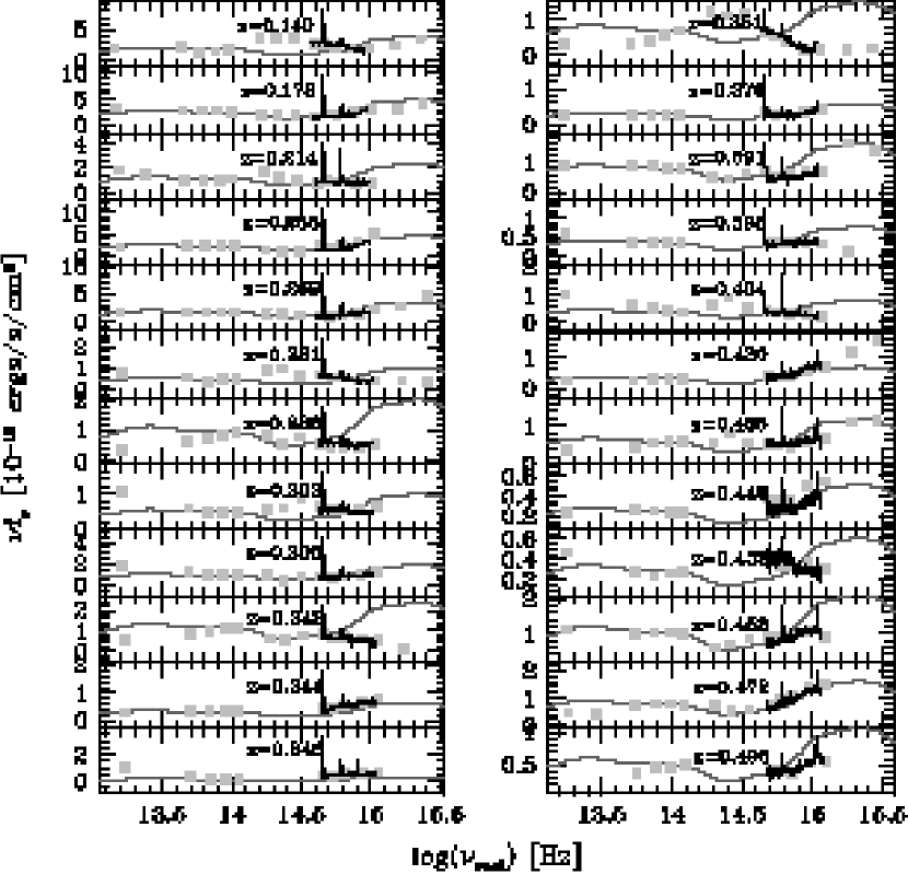
Figure 14: Individual mid-IR through UV SEDs for the quasars in our sample. The objects are ordered and labeled by redshift to correspond with the entries in Tables Spectral Energy Distributions and Multiwavelength Selection of Type 1 Quasars and Spectral Energy Distributions and Multiwavelength Selection of Type 1 Quasars. The black curve shows the SDSS spectrum (scaled by the average magnitude difference between the $g$-, $r$-, and $i$-band point-spread-function and fiber magnitudes to correct for fiber losses). The gray curve is the Elvis et al. (1994) mean radio-quiet SED (normalized to the 3.6$\mu$m point). The lighter gray symbols are the available broad-band photometric measurements for these objects from Spitzer-MIPS, ISO, Spitzer-IRAC, 2MASS, SDSS, and GALEX. No host galaxy correction has been applied.

Figures 14 through 24 present the individual SEDs of each of the 259 quasars in our sample. The plots are ordered by redshift to match Tables Spectral Energy Distributions and Multiwavelength Selection of Type 1 Quasars and Spectral Energy Distributions and Multiwavelength Selection of Type 1 Quasars. The individual data points are shown by gray squares. These are the observed values; host galaxy contamination has not been removed. The SDSS spectra are shown as solid black lines (smoothed by a 15 pixel boxcar). The SDSS spectra have been scaled by the difference between the $g$, $r$, and $i$ band PSF and fiber (3$\farcs$0) magnitudes to account for light losses due to the finite size of the optical fibers. The Elvis et al. (1994) radio-quiet mean SED is shown by the gray curves and is normalized to the 3.6$\mu$m data point of each quasar.

Figure 13: Histogram of bolometric corrections (from 5100Å to 100$\mu m$–10 keV) for our sample. According to our data, the bolometric correction (and thus the accretion rate) is overestimated by 17% on the average if the Elvis et al. (1994) RQ SED is assumed to apply to all quasars. Individual objects can have their bolometric corrections mis-estimated by up to a factor of 2 when assuming a mean SED.

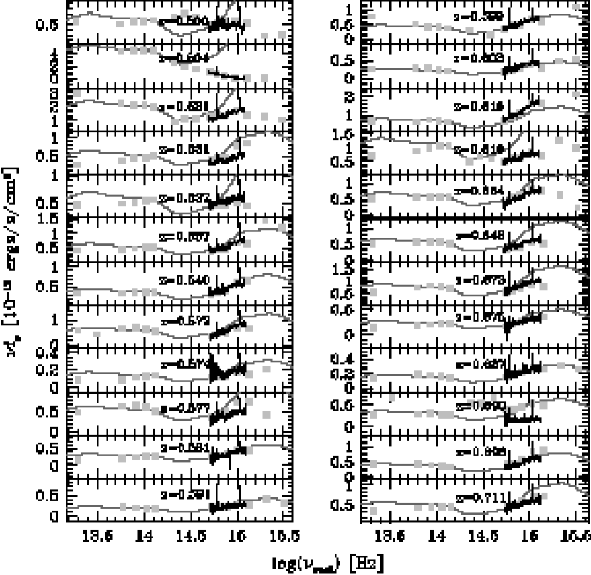
Figure 15: Same as for Fig. 14.

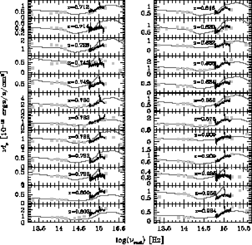
Figure 16: Same as for Fig. 14.

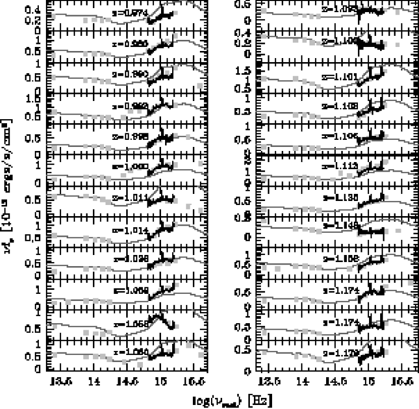
Figure 17: Same as for Fig. 14.

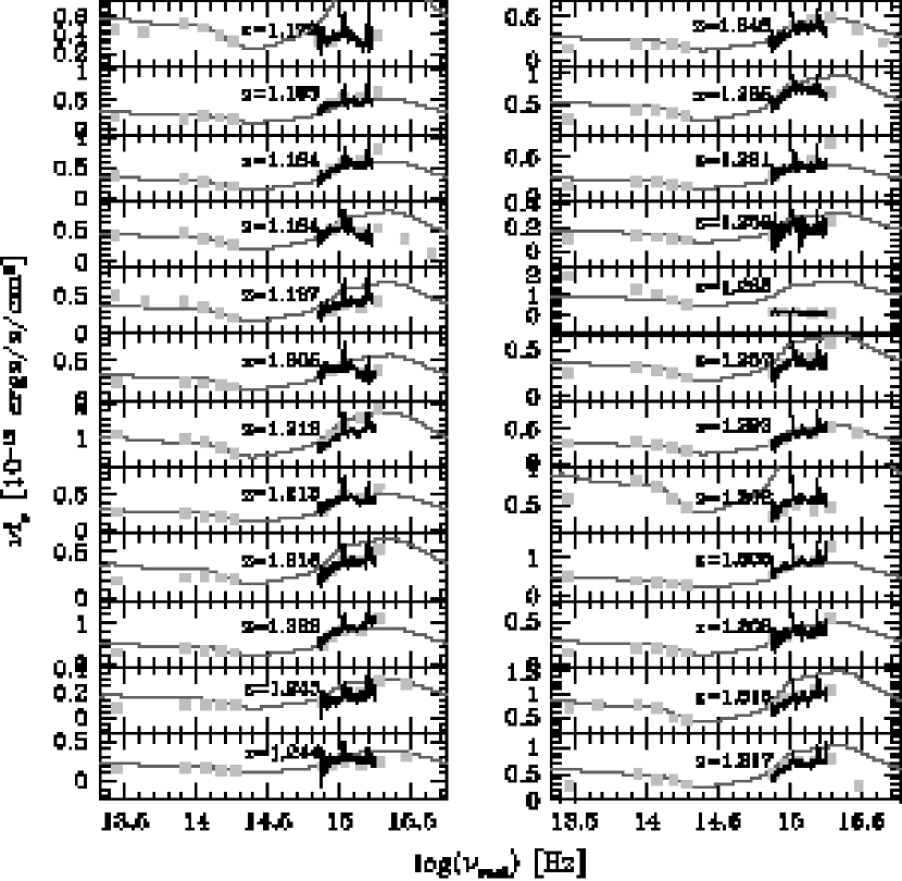
Figure 18: Same as for Fig. 14.

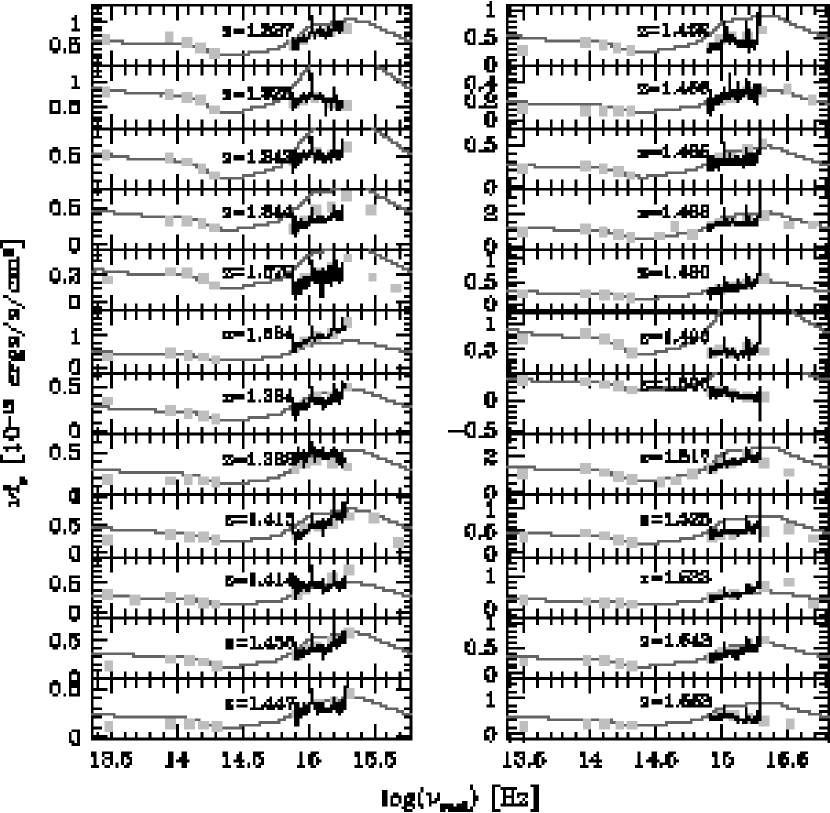
Figure 19: Same as for Fig. 14.

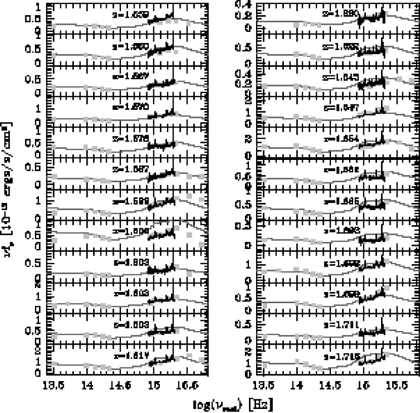
Figure 20: Same as for Fig. 14.

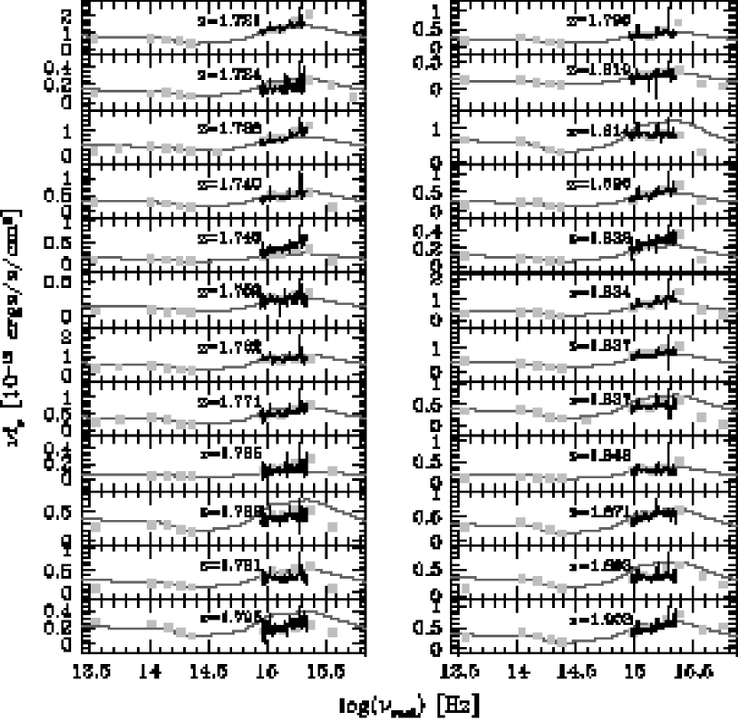
Figure 21: Same as for Fig. 14.

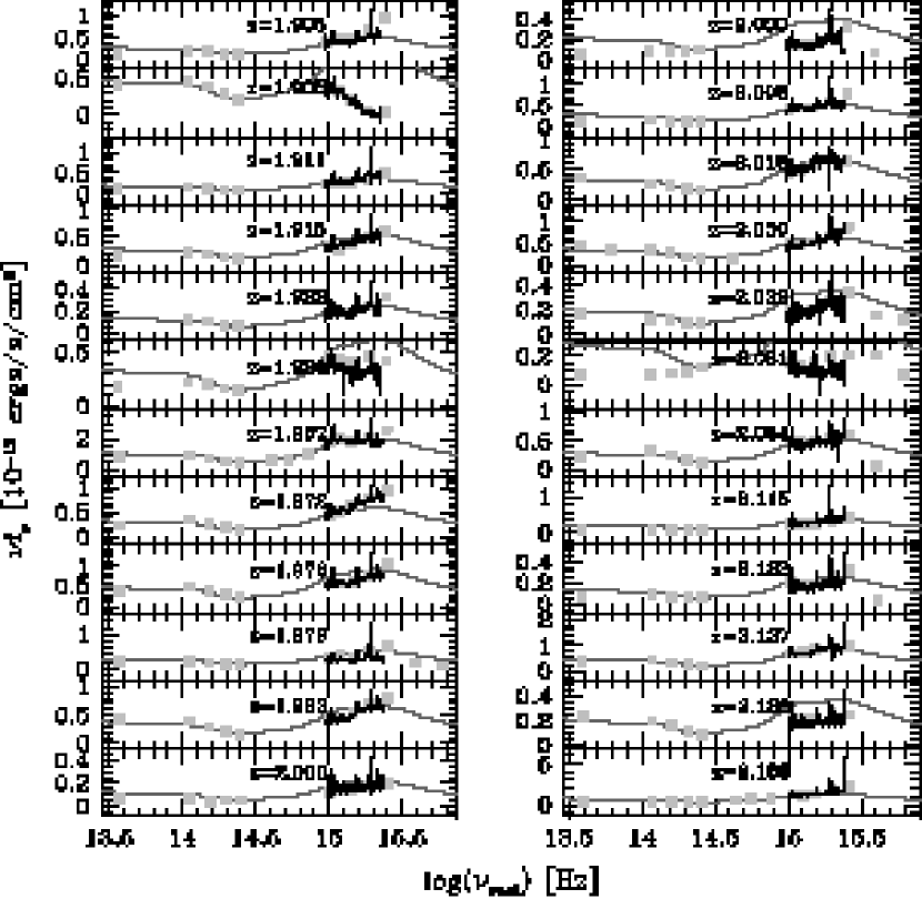
Figure 22: Same as for Fig. 14.

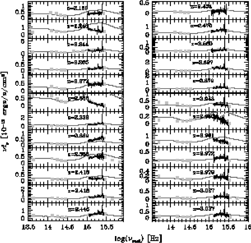
Figure 23: Same as for Fig. 14.

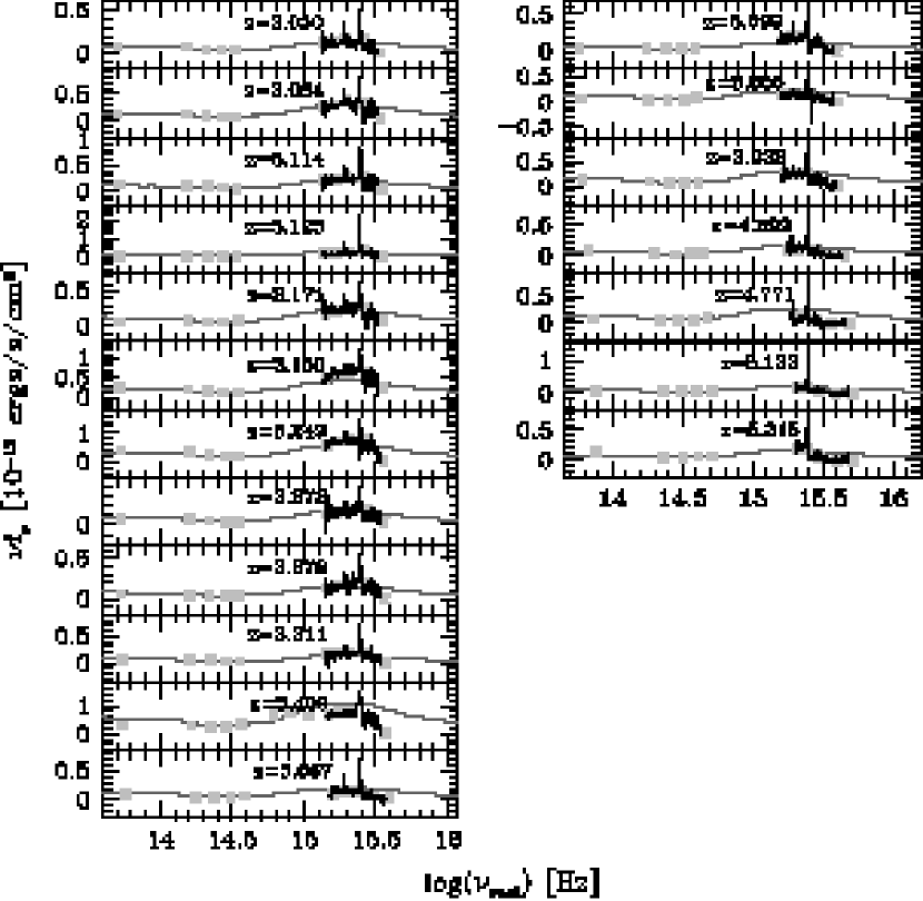
Figure 24: Same as for Fig. 14.

Table 1: SDSS-Spitzer Quasar Photometry I

Name	$z_{em}$	$L_{\rm bol}$	$L_{\rm opt}$	$L_{\rm ir}$	BC	X-ray	$f$	$n$	$u$	$g$	$r$	$i$	$z$
(SDSS J)		lg(ergs/s)	lg(ergs/s)	lg(ergs/s)		lg(c/s)	(AB mag)	(AB mag)	(AB mag)	(AB mag)	(AB mag)	(AB mag)	(AB mag)
105705.39+580437.4	0.140	45.06	44.49	44.78	10.60	-0.708	18.31$\pm$0.08	18.15$\pm$0.04	17.92$\pm$0.03	17.61$\pm$0.05	17.25$\pm$0.02	16.83$\pm$0.02	16.56$\pm$0.04
171902.28+593715.9	0.178	45.21	44.74	44.93	9.41	-1.221	18.10$\pm$0.01	17.99$\pm$0.01	17.49$\pm$0.02	17.50$\pm$0.02	17.36$\pm$0.02	17.06$\pm$0.02	17.20$\pm$0.02
160655.34+534016.8	0.214	45.13	44.45	44.91	11.87	$\ldots$	$\ldots$	$\ldots$	18.85$\pm$0.03	18.71$\pm$0.02	18.22$\pm$0.02	17.86$\pm$0.02	17.91$\pm$0.03
163111.28+404805.2	0.258	45.68	45.27	45.19	9.84	-0.551	$\ldots$	$\ldots$	16.98$\pm$0.01	17.05$\pm$0.02	17.08$\pm$0.01	17.10$\pm$0.01	16.86$\pm$0.01
171207.44+584754.4	0.269	45.49	45.06	45.12	12.29	-1.235	17.97$\pm$0.01	18.08$\pm$0.01	17.83$\pm$0.02	17.93$\pm$0.02	17.88$\pm$0.02	17.94$\pm$0.02	17.51$\pm$0.02
171033.21+584456.8	0.281	45.15	44.46	44.95	10.44	$\ldots$	20.59$\pm$0.04	20.06$\pm$0.02	19.58$\pm$0.03	19.25$\pm$0.03	18.70$\pm$0.02	18.52$\pm$0.02	18.10$\pm$0.03
105644.52+572233.4	0.286	45.08	44.53	44.78	10.12	$\ldots$	$\ldots$	$\ldots$	19.36$\pm$0.03	19.26$\pm$0.02	18.88$\pm$0.02	18.69$\pm$0.02	18.32$\pm$0.02
104739.49+563507.2	0.303	45.19	44.66	44.88	9.82	$\ldots$	$\ldots$	$\ldots$	19.16$\pm$0.04	19.02$\pm$0.04	18.72$\pm$0.04	18.57$\pm$0.03	18.20$\pm$0.03
155936.13+544203.8	0.308	45.42	44.87	45.15	11.75	$\ldots$	$\ldots$	$\ldots$	18.55$\pm$0.03	18.42$\pm$0.04	18.27$\pm$0.02	18.38$\pm$0.03	17.87$\pm$0.03
105626.96+580843.1	0.342	45.29	44.66	45.03	8.40	$\ldots$	$\ldots$	21.50$\pm$0.20	19.45$\pm$0.03	18.95$\pm$0.02	18.57$\pm$0.03	18.46$\pm$0.02	17.88$\pm$0.02
164343.24+405654.4	0.344	45.13	44.80	44.63	6.94	-1.683	$\ldots$	$\ldots$	18.92$\pm$0.02	18.82$\pm$0.01	18.72$\pm$0.02	18.75$\pm$0.02	18.55$\pm$0.03
104132.48+565953.1	0.346	45.37	44.75	45.13	13.08	$\ldots$	$\ldots$	$\ldots$	19.11$\pm$0.03	19.04$\pm$0.02	18.80$\pm$0.02	18.85$\pm$0.02	18.49$\pm$0.03
172052.30+590153.7	0.351	45.09	44.52	44.91	6.73	-1.959	21.42$\pm$0.03	21.18$\pm$0.03	20.84$\pm$0.09	20.41$\pm$0.03	19.07$\pm$0.02	18.60$\pm$0.02	18.21$\pm$0.03
105338.94+564135.1	0.379	45.10	44.65	44.64	9.10	-1.397	$\ldots$	$\ldots$	19.57$\pm$0.04	19.56$\pm$0.04	19.42$\pm$0.04	19.22$\pm$0.03	18.91$\pm$0.04
104705.07+590728.4	0.391	45.54	45.06	45.20	12.32	$\ldots$	19.28$\pm$0.13	18.65$\pm$0.05	19.10$\pm$0.03	18.76$\pm$0.03	18.72$\pm$0.03	18.55$\pm$0.02	18.04$\pm$0.04
103753.15+573507.8	0.398	45.21	44.61	44.93	8.35	$\ldots$	$\ldots$	21.08$\pm$0.17	19.91$\pm$0.04	19.41$\pm$0.04	19.16$\pm$0.02	19.00$\pm$0.02	18.79$\pm$0.04
163308.28+403321.4	0.404	45.34	44.59	45.19	11.81	$\ldots$	$\ldots$	$\ldots$	20.46$\pm$0.06	19.77$\pm$0.02	19.37$\pm$0.02	19.03$\pm$0.02	18.71$\pm$0.04
105308.24+590522.2	0.430	45.43	45.06	44.82	11.54	$\ldots$	19.17$\pm$0.12	19.05$\pm$0.07	19.10$\pm$0.03	18.93$\pm$0.04	19.06$\pm$0.01	19.03$\pm$0.02	18.71$\pm$0.04
105141.16+591305.2	0.435	45.50	45.07	45.08	10.26	$\ldots$	19.49$\pm$0.14	19.07$\pm$0.07	19.17$\pm$0.04	18.95$\pm$0.03	18.98$\pm$0.02	18.70$\pm$0.03	18.42$\pm$0.03
104405.38+570024.2	0.448	45.30	44.90	44.80	7.80	$\ldots$	$\ldots$	$\ldots$	19.35$\pm$0.03	19.18$\pm$0.02	19.21$\pm$0.02	19.00$\pm$0.03	18.80$\pm$0.04
105639.42+575721.4	0.453	45.29	44.76	44.95	8.00	-1.400	$\ldots$	$\ldots$	20.01$\pm$0.06	19.51$\pm$0.03	19.27$\pm$0.02	19.07$\pm$0.02	18.73$\pm$0.05
105959.93+574848.1	0.453	45.72	45.21	45.43	8.26	$\ldots$	$\ldots$	$\ldots$	18.82$\pm$0.03	18.36$\pm$0.03	18.25$\pm$0.02	18.05$\pm$0.02	17.81$\pm$0.02
163502.80+412952.9	0.472	45.77	45.37	45.25	7.92	-0.975	$\ldots$	$\ldots$	18.29$\pm$0.02	18.03$\pm$0.02	18.07$\pm$0.01	17.99$\pm$0.02	17.97$\pm$0.02
103120.10+581851.0	0.493	45.49	45.02	45.13	8.46	$\ldots$	$\ldots$	$\ldots$	19.39$\pm$0.03	19.10$\pm$0.03	19.14$\pm$0.02	18.87$\pm$0.02	18.62$\pm$0.04
103651.94+575950.9	0.500	45.56	45.02	45.30	7.32	$\ldots$	20.93$\pm$0.28	20.54$\pm$0.13	19.43$\pm$0.03	19.02$\pm$0.02	18.75$\pm$0.02	18.58$\pm$0.02	18.46$\pm$0.04
103039.62+580611.5	0.504	46.25	45.04	46.21	23.81	$\ldots$	$\ldots$	22.72$\pm$0.37	21.69$\pm$0.17	20.36$\pm$0.04	19.10$\pm$0.02	18.14$\pm$0.01	17.62$\pm$0.02
171352.41+584201.2	0.521	46.17	45.50	46.00	10.42	$\ldots$	19.59$\pm$0.03	18.91$\pm$0.01	18.31$\pm$0.03	17.85$\pm$0.01	17.79$\pm$0.01	17.51$\pm$0.01	17.48$\pm$0.03
163031.46+410145.6	0.531	45.60	45.23	45.17	8.34	-1.632	$\ldots$	$\ldots$	18.89$\pm$0.02	18.70$\pm$0.02	18.89$\pm$0.01	18.73$\pm$0.02	18.66$\pm$0.03
163143.76+404735.6	0.537	45.60	45.08	45.30	7.79	$\ldots$	$\ldots$	$\ldots$	19.56$\pm$0.03	19.13$\pm$0.02	18.96$\pm$0.01	18.69$\pm$0.02	18.65$\pm$0.03
171126.94+585544.2	0.537	45.69	45.29	45.27	10.12	-1.660	19.47$\pm$0.02	18.80$\pm$0.01	19.17$\pm$0.03	18.80$\pm$0.02	18.92$\pm$0.02	18.77$\pm$0.02	18.71$\pm$0.05
104556.84+570747.0	0.540	45.57	45.15	45.14	9.42	$\ldots$	$\ldots$	$\ldots$	19.15$\pm$0.03	18.93$\pm$0.02	19.05$\pm$0.02	18.98$\pm$0.03	18.96$\pm$0.04
160523.10+545613.3	0.572	45.80	45.24	45.42	11.68	-1.006	$\ldots$	$\ldots$	19.12$\pm$0.04	18.82$\pm$0.04	18.90$\pm$0.03	18.75$\pm$0.02	18.80$\pm$0.05
103333.92+582818.8	0.574	45.11	44.65	44.68	8.42	$\ldots$	$\ldots$	20.89$\pm$0.20	20.77$\pm$0.07	20.28$\pm$0.03	20.40$\pm$0.04	20.20$\pm$0.05	20.04$\pm$0.14
104625.02+584839.1	0.577	45.74	45.22	45.42	9.56	$\ldots$	$\ldots$	20.10$\pm$0.12	19.03$\pm$0.02	18.74$\pm$0.03	18.83$\pm$0.03	18.70$\pm$0.02	18.77$\pm$0.04
160341.44+541501.5	0.581	45.47	45.08	44.99	7.70	$\ldots$	$\ldots$	$\ldots$	19.59$\pm$0.05	19.25$\pm$0.02	19.30$\pm$0.03	19.19$\pm$0.03	19.14$\pm$0.05
103157.05+581609.9	0.591	45.43	44.97	45.03	8.25	-1.609	20.84$\pm$0.28	20.17$\pm$0.11	20.07$\pm$0.05	19.70$\pm$0.04	19.72$\pm$0.03	19.39$\pm$0.03	19.36$\pm$0.06
171736.90+593011.4	0.599	45.83	45.36	45.47	11.85	$\ldots$	19.52$\pm$0.01	18.83$\pm$0.01	19.25$\pm$0.03	18.82$\pm$0.02	18.91$\pm$0.02	18.75$\pm$0.02	18.85$\pm$0.04
103721.15+590755.7	0.603	45.52	45.04	45.13	11.48	$\ldots$	20.32$\pm$0.27	19.99$\pm$0.13	20.05$\pm$0.15	19.42$\pm$0.03	19.58$\pm$0.02	19.46$\pm$0.02	19.64$\pm$0.10
171334.02+595028.3	0.615	46.08	45.73	45.56	9.94	$\ldots$	18.83$\pm$0.01	18.11$\pm$0.01	18.18$\pm$0.02	17.89$\pm$0.01	18.01$\pm$0.02	17.97$\pm$0.02	18.14$\pm$0.03
171117.66+584123.8	0.616	45.97	45.47	45.67	10.50	$\ldots$	19.66$\pm$0.03	18.93$\pm$0.01	19.09$\pm$0.03	18.60$\pm$0.02	18.60$\pm$0.02	18.35$\pm$0.02	18.43$\pm$0.04
171818.14+584905.2	0.634	45.90	45.35	45.67	10.32	$\ldots$	21.19$\pm$0.08	19.67$\pm$0.02	19.02$\pm$0.03	18.59$\pm$0.02	18.59$\pm$0.02	18.51$\pm$0.02	18.66$\pm$0.04
104526.73+595422.6	0.646	45.81	45.27	45.54	9.98	$\ldots$	$\ldots$	$\ldots$	19.42$\pm$0.04	19.06$\pm$0.03	19.14$\pm$0.02	18.84$\pm$0.03	18.83$\pm$0.05
160015.68+552259.9	0.673	45.99	45.51	45.67	8.93	$\ldots$	$\ldots$	$\ldots$	18.92$\pm$0.03	18.53$\pm$0.02	18.53$\pm$0.01	18.41$\pm$0.02	18.34$\pm$0.04
104210.25+594253.5	0.675	45.51	45.09	45.07	10.00	$\ldots$	$\ldots$	$\ldots$	19.84$\pm$0.09	19.66$\pm$0.04	19.65$\pm$0.02	19.63$\pm$0.04	19.69$\pm$0.12
103236.22+580033.9	0.687	45.48	45.03	45.05	9.34	-1.703	21.11$\pm$0.31	20.45$\pm$0.13	20.19$\pm$0.05	19.83$\pm$0.03	19.81$\pm$0.03	19.62$\pm$0.03	19.78$\pm$0.08
163915.80+412833.7	0.690	45.83	45.41	45.44	8.56	$\ldots$	$\ldots$	$\ldots$	19.48$\pm$0.03	19.11$\pm$0.02	19.02$\pm$0.01	18.89$\pm$0.01	18.71$\pm$0.04
105518.08+570423.5	0.696	45.92	45.52	45.48	9.43	$\ldots$	$\ldots$	$\ldots$	18.87$\pm$0.02	18.59$\pm$0.02	18.71$\pm$0.01	18.72$\pm$0.02	18.68$\pm$0.04
163854.62+415419.5	0.711	45.89	45.50	45.50	8.10	-1.743	$\ldots$	$\ldots$	19.06$\pm$0.05	18.79$\pm$0.02	18.68$\pm$0.02	18.62$\pm$0.02	18.61$\pm$0.04
104633.70+571530.4	0.712	45.89	45.50	45.41	9.10	$\ldots$	$\ldots$	$\ldots$	18.98$\pm$0.02	18.70$\pm$0.01	18.76$\pm$0.02	18.75$\pm$0.01	18.75$\pm$0.03
104840.28+563635.6	0.714	45.78	45.31	45.45	8.08	$\ldots$	$\ldots$	$\ldots$	19.65$\pm$0.04	19.22$\pm$0.03	19.18$\pm$0.02	19.04$\pm$0.02	18.89$\pm$0.04
160128.54+544521.3	0.728	46.35	45.78	46.12	12.55	$\ldots$	$\ldots$	$\ldots$	18.36$\pm$0.02	18.12$\pm$0.02	18.06$\pm$0.02	18.05$\pm$0.02	18.00$\pm$0.03
172414.05+593644.0	0.745	45.83	45.43	45.50	5.87	$\ldots$	22.10$\pm$0.05	20.08$\pm$0.01	19.32$\pm$0.03	18.90$\pm$0.02	18.80$\pm$0.01	18.77$\pm$0.02	18.55$\pm$0.03
163135.46+405756.4	0.749	45.95	45.43	45.67	8.95	$\ldots$	$\ldots$	$\ldots$	19.49$\pm$0.03	19.02$\pm$0.01	18.86$\pm$0.02	18.87$\pm$0.02	18.70$\pm$0.04
163709.32+414030.8	0.760	46.56	46.18	46.18	8.83	-1.561	$\ldots$	$\ldots$	17.67$\pm$0.02	17.13$\pm$0.01	17.19$\pm$0.01	17.30$\pm$0.02	17.21$\pm$0.02
171748.43+594820.6	0.763	46.12	45.81	45.67	6.84	$\ldots$	20.62$\pm$0.02	18.58$\pm$0.01	18.30$\pm$0.03	17.99$\pm$0.02	18.02$\pm$0.02	18.10$\pm$0.02	18.06$\pm$0.03
105106.12+591625.1	0.768	46.14	45.74	45.86	7.96	-1.624	20.91$\pm$0.28	19.00$\pm$0.06	18.58$\pm$0.03	18.20$\pm$0.03	18.25$\pm$0.02	18.30$\pm$0.02	18.16$\pm$0.03
163352.34+402115.5	0.782	45.93	45.51	45.58	9.10	-1.936	$\ldots$	$\ldots$	19.23$\pm$0.03	18.87$\pm$0.02	18.95$\pm$0.02	19.11$\pm$0.02	18.90$\pm$0.04
172104.75+592451.4	0.786	45.93	45.44	45.60	11.18	$\ldots$	20.26$\pm$0.02	19.47$\pm$0.01	19.63$\pm$0.04	19.39$\pm$0.02	19.32$\pm$0.02	19.34$\pm$0.03	19.13$\pm$0.06
104857.92+560112.3	0.800	45.89	45.56	45.28	7.14	$\ldots$	$\ldots$	$\ldots$	19.13$\pm$0.03	18.81$\pm$0.04	18.82$\pm$0.01	18.94$\pm$0.02	18.76$\pm$0.04
110116.41+572850.5	0.803	46.44	46.10	45.94	7.23	$\ldots$	$\ldots$	$\ldots$	17.81$\pm$0.02	17.50$\pm$0.01	17.46$\pm$0.01	17.45$\pm$0.01	17.39$\pm$0.02
160908.95+533153.2	0.816	46.10	45.68	45.72	8.57	$\ldots$	$\ldots$	$\ldots$	19.00$\pm$0.03	18.47$\pm$0.03	18.45$\pm$0.04	18.66$\pm$0.02	18.48$\pm$0.03
160630.60+542007.5	0.820	46.17	45.65	45.90	11.06	$\ldots$	$\ldots$	$\ldots$	18.99$\pm$0.03	18.74$\pm$0.03	18.71$\pm$0.02	18.81$\pm$0.03	18.60$\pm$0.04
105604.00+581523.4	0.832	46.10	45.69	45.73	10.57	$\ldots$	20.28$\pm$0.21	18.86$\pm$0.06	18.96$\pm$0.03	18.87$\pm$0.02	18.80$\pm$0.03	18.91$\pm$0.02	18.76$\pm$0.03
105000.21+581904.2	0.833	46.44	46.09	45.93	8.57	$\ldots$	$\ldots$	$\ldots$	17.81$\pm$0.01	17.63$\pm$0.01	17.62$\pm$0.02	17.75$\pm$0.01	17.67$\pm$0.03
164311.83+405043.2	0.834	46.01	45.57	45.63	8.37	$\ldots$	$\ldots$	$\ldots$	19.27$\pm$0.03	19.00$\pm$0.02	18.89$\pm$0.02	18.94$\pm$0.02	18.75$\pm$0.04
163726.88+404432.9	0.858	46.24	45.85	45.80	10.04	$\ldots$	$\ldots$	$\ldots$	18.46$\pm$0.02	18.41$\pm$0.01	18.43$\pm$0.01	18.53$\pm$0.02	18.44$\pm$0.03
160623.56+540555.8	0.876	46.54	46.18	46.10	8.71	-1.580	$\ldots$	$\ldots$	17.91$\pm$0.02	17.64$\pm$0.02	17.59$\pm$0.03	17.66$\pm$0.02	17.64$\pm$0.03
104355.47+593054.0	0.909	45.68	45.26	45.17	11.62	$\ldots$	20.87$\pm$0.31	19.68$\pm$0.10	20.89$\pm$0.10	20.38$\pm$0.03	20.30$\pm$0.03	20.40$\pm$0.04	20.11$\pm$0.15
163225.56+411852.4	0.909	46.29	45.88	45.89	9.46	$\ldots$	$\ldots$	$\ldots$	18.59$\pm$0.02	18.45$\pm$0.02	18.38$\pm$0.01	18.41$\pm$0.01	18.36$\pm$0.03
103829.74+585204.1	0.935	45.88	45.33	45.62	9.58	$\ldots$	$\ldots$	20.86$\pm$0.19	20.33$\pm$0.06	19.91$\pm$0.02	19.54$\pm$0.03	19.61$\pm$0.03	19.48$\pm$0.09
103855.33+575814.7	0.956	46.37	45.85	46.03	10.46	$\ldots$	19.44$\pm$0.14	19.16$\pm$0.08	19.16$\pm$0.03	18.84$\pm$0.03	18.53$\pm$0.02	18.55$\pm$0.02	18.42$\pm$0.03
103525.05+580335.6	0.964	46.06	45.74	45.43	10.01	$\ldots$	20.22$\pm$0.21	19.42$\pm$0.08	18.94$\pm$0.02	19.03$\pm$0.02	18.93$\pm$0.03	19.05$\pm$0.02	19.13$\pm$0.04
163306.12+401747.4	0.974	45.93	45.44	45.60	10.56	$\ldots$	$\ldots$	$\ldots$	19.88$\pm$0.04	19.76$\pm$0.02	19.63$\pm$0.02	19.85$\pm$0.02	19.54$\pm$0.06
171145.53+601318.5	0.980	46.32	45.97	45.79	8.94	$\ldots$	$\ldots$	$\ldots$	18.48$\pm$0.02	18.48$\pm$0.02	18.34$\pm$0.02	18.39$\pm$0.02	18.39$\pm$0.04
172310.35+595105.6	0.990	46.22	45.88	45.89	9.73	-2.215	21.27$\pm$0.03	18.73$\pm$0.01	18.86$\pm$0.03	18.84$\pm$0.02	18.69$\pm$0.02	18.89$\pm$0.02	18.75$\pm$0.04
160913.18+535429.6	0.992	46.46	46.08	46.06	7.37	-1.706	$\ldots$	$\ldots$	18.56$\pm$0.03	18.30$\pm$0.02	18.00$\pm$0.02	17.97$\pm$0.02	17.99$\pm$0.03
104239.66+583231.0	0.998	46.07	45.68	45.60	9.10	$\ldots$	$\ldots$	19.88$\pm$0.11	19.28$\pm$0.03	19.21$\pm$0.02	18.98$\pm$0.02	19.06$\pm$0.02	19.08$\pm$0.04
172130.96+584404.7	1.000	46.35	46.07	45.65	6.68	$\ldots$	19.58$\pm$0.01	18.52$\pm$0.01	18.68$\pm$0.02	18.43$\pm$0.01	18.22$\pm$0.01	18.25$\pm$0.02	18.33$\pm$0.03
104930.46+592032.6	1.011	46.24	45.69	46.04	8.31	$\ldots$	21.67$\pm$0.39	20.62$\pm$0.13	19.56$\pm$0.03	19.22$\pm$0.02	18.89$\pm$0.02	18.80$\pm$0.02	18.59$\pm$0.05
104859.67+565648.6	1.014	46.37	45.96	45.96	10.26	$\ldots$	$\ldots$	$\ldots$	18.65$\pm$0.03	18.47$\pm$0.02	18.35$\pm$0.02	18.47$\pm$0.01	18.50$\pm$0.03
104659.37+573055.8	1.026	46.13	45.73	45.61	9.27	-1.445	$\ldots$	$\ldots$	19.30$\pm$0.03	19.20$\pm$0.02	18.87$\pm$0.02	18.89$\pm$0.02	19.02$\pm$0.04
163930.82+410013.6	1.052	46.37	46.05	45.70	8.85	$\ldots$	$\ldots$	$\ldots$	18.46$\pm$0.02	18.33$\pm$0.02	18.20$\pm$0.02	18.27$\pm$0.01	18.45$\pm$0.03
104935.76+554950.5	1.056	46.34	45.94	45.96	5.59	$\ldots$	$\ldots$	$\ldots$	19.31$\pm$0.04	18.85$\pm$0.04	18.21$\pm$0.04	18.06$\pm$0.04	17.98$\pm$0.04
171732.94+594747.5	1.060	46.40	45.90	46.10	16.44	$\ldots$	20.29$\pm$0.02	19.21$\pm$0.01	19.02$\pm$0.03	18.86$\pm$0.03	18.59$\pm$0.02	18.61$\pm$0.02	18.66$\pm$0.04
104114.18+590219.4	1.093	46.03	45.59	45.65	6.38	$\ldots$	$\ldots$	20.67$\pm$0.16	20.01$\pm$0.04	19.78$\pm$0.02	19.25$\pm$0.02	19.16$\pm$0.02	18.99$\pm$0.06
104156.51+593611.2	1.100	46.01	45.42	45.79	11.05	$\ldots$	$\ldots$	21.10$\pm$0.20	20.55$\pm$0.13	20.26$\pm$0.04	19.76$\pm$0.03	19.68$\pm$0.04	19.64$\pm$0.11
105404.10+574019.7	1.101	46.67	46.18	46.35	12.12	$\ldots$	$\ldots$	$\ldots$	18.29$\pm$0.02	18.19$\pm$0.02	18.03$\pm$0.01	18.07$\pm$0.02	18.11$\pm$0.02
104757.52+573451.8	1.102	46.30	45.86	45.91	12.81	$\ldots$	$\ldots$	$\ldots$	19.03$\pm$0.02	19.06$\pm$0.01	18.83$\pm$0.01	18.92$\pm$0.01	19.09$\pm$0.05
104921.49+575036.6	1.106	46.19	45.84	45.64	6.91	$\ldots$	$\ldots$	$\ldots$	19.25$\pm$0.03	19.04$\pm$0.03	18.78$\pm$0.02	18.73$\pm$0.03	18.70$\pm$0.04
105239.60+572431.4	1.112	46.58	46.28	45.92	8.42	$\ldots$	$\ldots$	$\ldots$	18.07$\pm$0.03	18.01$\pm$0.02	17.77$\pm$0.01	17.71$\pm$0.01	17.81$\pm$0.02
163210.88+405503.1	1.136	46.18	45.82	45.61	8.42	$\ldots$	$\ldots$	$\ldots$	19.24$\pm$0.03	19.22$\pm$0.01	18.98$\pm$0.02	18.94$\pm$0.02	19.03$\pm$0.05
104539.27+580711.0	1.149	46.10	45.32	45.95	24.88	$\ldots$	$\ldots$	21.14$\pm$0.23	20.75$\pm$0.07	20.54$\pm$0.03	20.34$\pm$0.03	20.24$\pm$0.03	20.45$\pm$0.14
163531.05+410027.3	1.152	46.35	45.92	45.95	10.50	$\ldots$	$\ldots$	$\ldots$	19.07$\pm$0.03	19.01$\pm$0.01	18.79$\pm$0.02	18.83$\pm$0.02	18.88$\pm$0.03
105310.16+585532.7	1.174	46.35	45.96	45.81	11.93	$\ldots$	19.87$\pm$0.17	19.00$\pm$0.06	19.09$\pm$0.02	19.14$\pm$0.02	18.83$\pm$0.02	18.92$\pm$0.02	19.01$\pm$0.04
163844.49+410529.0	1.174	46.30	45.91	45.87	7.96	$\ldots$	$\ldots$	$\ldots$	19.25$\pm$0.03	19.13$\pm$0.02	18.80$\pm$0.02	18.68$\pm$0.01	18.66$\pm$0.04
163618.51+415058.9	1.179	46.29	45.79	46.00	12.30	$\ldots$	$\ldots$	$\ldots$	19.61$\pm$0.04	19.32$\pm$0.02	19.06$\pm$0.02	19.04$\pm$0.02	19.18$\pm$0.06
163702.20+413022.2	1.179	46.33	45.80	46.07	6.90	$\ldots$	$\ldots$	$\ldots$	19.74$\pm$0.03	19.67$\pm$0.02	19.08$\pm$0.02	19.13$\pm$0.02	18.95$\pm$0.04
163208.52+403310.4	1.183	46.26	45.90	45.72	8.23	$\ldots$	$\ldots$	$\ldots$	19.16$\pm$0.02	19.12$\pm$0.02	18.82$\pm$0.01	18.73$\pm$0.02	18.83$\pm$0.04
104551.80+562203.5	1.184	46.38	45.98	45.92	9.85	$\ldots$	$\ldots$	$\ldots$	18.93$\pm$0.05	18.91$\pm$0.03	18.72$\pm$0.03	18.68$\pm$0.03	18.74$\pm$0.04
172041.40+593244.3	1.184	46.31	45.87	46.03	8.51	$\ldots$	21.80$\pm$0.04	20.25$\pm$0.01	19.39$\pm$0.03	19.26$\pm$0.02	18.70$\pm$0.02	18.63$\pm$0.02	18.75$\pm$0.04
160250.95+545057.8	1.197	46.32	45.76	46.06	12.66	$\ldots$	$\ldots$	$\ldots$	19.63$\pm$0.04	19.52$\pm$0.03	19.19$\pm$0.03	19.16$\pm$0.02	19.18$\pm$0.07
105316.75+573550.8	1.205	46.20	45.79	45.80	7.53	$\ldots$	$\ldots$	$\ldots$	19.72$\pm$0.04	19.59$\pm$0.02	19.06$\pm$0.02	18.94$\pm$0.02	18.93$\pm$0.04
160953.03+533443.8	1.212	46.80	46.36	46.44	12.10	$\ldots$	$\ldots$	$\ldots$	18.04$\pm$0.03	17.91$\pm$0.02	17.80$\pm$0.02	17.86$\pm$0.02	17.95$\pm$0.03
163529.60+400503.6	1.213	46.27	45.87	45.81	10.51	$\ldots$	$\ldots$	$\ldots$	19.28$\pm$0.03	19.28$\pm$0.02	18.90$\pm$0.02	18.95$\pm$0.02	19.14$\pm$0.05
160100.07+551104.8	1.216	46.23	45.82	45.78	11.74	$\ldots$	$\ldots$	$\ldots$	19.38$\pm$0.04	19.41$\pm$0.03	19.10$\pm$0.02	19.19$\pm$0.03	19.36$\pm$0.07
104719.20+582117.5	1.222	46.53	46.16	46.01	10.45	$\ldots$	$\ldots$	$\ldots$	18.57$\pm$0.02	18.59$\pm$0.03	18.34$\pm$0.02	18.33$\pm$0.01	18.52$\pm$0.03
103222.85+575551.1	1.243	45.98	45.56	45.50	10.90	$\ldots$	$\ldots$	20.61$\pm$0.14	20.03$\pm$0.05	20.16$\pm$0.03	19.95$\pm$0.03	20.03$\pm$0.04	19.99$\pm$0.09
103653.00+584734.2	1.244	46.04	45.61	45.65	8.73	$\ldots$	$\ldots$	20.53$\pm$0.17	20.21$\pm$0.05	20.19$\pm$0.03	19.66$\pm$0.03	19.68$\pm$0.03	19.58$\pm$0.10
105045.59+591940.4	1.248	46.15	45.80	45.68	9.51	$\ldots$	21.36$\pm$0.34	20.33$\pm$0.12	19.49$\pm$0.04	19.29$\pm$0.03	19.15$\pm$0.02	19.31$\pm$0.03	19.41$\pm$0.06
160429.01+544333.9	1.265	46.46	46.09	46.01	7.75	$\ldots$	$\ldots$	$\ldots$	19.12$\pm$0.04	18.75$\pm$0.02	18.38$\pm$0.02	18.35$\pm$0.02	18.38$\pm$0.03
105050.14+573820.0	1.281	46.28	45.92	45.66	10.17	$\ldots$	$\ldots$	$\ldots$	19.15$\pm$0.02	19.24$\pm$0.05	19.06$\pm$0.02	19.05$\pm$0.02	19.15$\pm$0.05
103841.94+571220.5	1.282	46.03	45.58	45.58	10.99	-1.719	$\ldots$	$\ldots$	20.23$\pm$0.05	20.27$\pm$0.03	19.70$\pm$0.02	19.75$\pm$0.03	19.85$\pm$0.08
103803.35+572701.6	1.285	46.83	45.54	46.79	64.41	$\ldots$	$\ldots$	$\ldots$	21.28$\pm$0.12	20.91$\pm$0.05	20.14$\pm$0.03	19.95$\pm$0.03	19.79$\pm$0.10
163835.82+411734.8	1.287	46.35	45.91	45.96	12.48	$\ldots$	$\ldots$	$\ldots$	19.31$\pm$0.03	19.34$\pm$0.02	19.01$\pm$0.02	19.04$\pm$0.02	19.19$\pm$0.05
104454.89+592134.1	1.292	46.34	45.89	45.97	10.78	$\ldots$	$\ldots$	20.10$\pm$0.12	19.39$\pm$0.06	19.34$\pm$0.02	19.01$\pm$0.03	19.09$\pm$0.03	19.07$\pm$0.06
161215.12+531247.7	1.302	46.56	45.96	46.36	14.32	$\ldots$	$\ldots$	$\ldots$	19.56$\pm$0.05	19.36$\pm$0.03	18.92$\pm$0.03	18.87$\pm$0.02	18.84$\pm$0.05
161338.23+531351.5	1.306	46.63	46.24	46.14	10.82	$\ldots$	$\ldots$	$\ldots$	18.43$\pm$0.02	18.49$\pm$0.02	18.24$\pm$0.02	18.27$\pm$0.02	18.39$\pm$0.03
164138.75+412232.3	1.308	46.26	45.89	45.74	8.59	$\ldots$	$\ldots$	$\ldots$	19.40$\pm$0.03	19.57$\pm$0.02	19.15$\pm$0.02	19.08$\pm$0.02	19.06$\pm$0.04
164018.34+405813.0	1.316	46.73	46.29	46.37	9.44	$\ldots$	$\ldots$	$\ldots$	18.62$\pm$0.02	18.30$\pm$0.02	18.11$\pm$0.02	18.04$\pm$0.01	18.02$\pm$0.03
103850.23+575137.0	1.317	46.50	46.10	46.10	8.32	$\ldots$	$\ldots$	20.57$\pm$0.16	18.99$\pm$0.04	18.70$\pm$0.02	18.41$\pm$0.02	18.32$\pm$0.02	18.44$\pm$0.04
160230.02+543658.5	1.327	46.64	46.16	46.32	11.90	$\ldots$	$\ldots$	$\ldots$	18.87$\pm$0.03	18.67$\pm$0.02	18.39$\pm$0.02	18.41$\pm$0.02	18.50$\pm$0.03
160943.67+533041.0	1.328	46.69	46.11	46.49	11.02	$\ldots$	$\ldots$	$\ldots$	19.36$\pm$0.04	18.97$\pm$0.02	18.51$\pm$0.02	18.36$\pm$0.02	18.29$\pm$0.03
104622.60+574034.2	1.343	46.54	46.05	46.23	10.37	$\ldots$	$\ldots$	$\ldots$	19.25$\pm$0.03	19.12$\pm$0.02	18.78$\pm$0.02	18.68$\pm$0.02	18.65$\pm$0.03
103301.50+583749.7	1.344	46.45	45.96	46.10	17.01	$\ldots$	$\ldots$	20.01$\pm$0.13	19.18$\pm$0.03	19.14$\pm$0.02	18.94$\pm$0.02	19.11$\pm$0.02	19.41$\pm$0.09
171948.31+592422.9	1.370	46.15	45.66	45.87	17.01	$\ldots$	22.14$\pm$0.05	21.02$\pm$0.02	19.92$\pm$0.05	19.89$\pm$0.03	19.80$\pm$0.02	19.80$\pm$0.04	20.13$\pm$0.12
104431.32+565316.6	1.384	46.70	46.34	46.15	10.27	$\ldots$	$\ldots$	$\ldots$	18.32$\pm$0.02	18.31$\pm$0.02	18.14$\pm$0.01	18.14$\pm$0.02	18.21$\pm$0.03
163759.16+420336.7	1.384	46.37	45.90	46.01	12.79	$\ldots$	$\ldots$	$\ldots$	19.50$\pm$0.06	19.46$\pm$0.02	19.20$\pm$0.02	19.20$\pm$0.02	19.27$\pm$0.06
104331.83+562943.8	1.392	46.28	45.90	45.83	7.80	$\ldots$	$\ldots$	$\ldots$	19.91$\pm$0.04	19.45$\pm$0.02	19.12$\pm$0.03	18.96$\pm$0.02	19.00$\pm$0.05
171815.96+584613.6	1.413	46.44	46.07	46.05	11.31	$\ldots$	21.40$\pm$0.10	19.69$\pm$0.02	19.17$\pm$0.03	19.07$\pm$0.03	18.88$\pm$0.02	18.82$\pm$0.03	19.02$\pm$0.05
163739.43+414348.0	1.414	46.48	46.07	46.01	12.13	$\ldots$	$\ldots$	$\ldots$	19.04$\pm$0.02	18.97$\pm$0.01	18.92$\pm$0.01	18.92$\pm$0.01	19.01$\pm$0.04
105014.96+562333.7	1.435	46.43	46.04	45.95	10.12	$\ldots$	$\ldots$	$\ldots$	19.25$\pm$0.05	19.18$\pm$0.03	19.06$\pm$0.02	18.94$\pm$0.02	18.96$\pm$0.04
105039.54+572336.6	1.447	46.31	45.93	45.78	9.57	$\ldots$	$\ldots$	$\ldots$	19.59$\pm$0.03	19.52$\pm$0.04	19.26$\pm$0.02	19.18$\pm$0.02	19.30$\pm$0.05
172353.33+600002.8	1.452	46.53	46.09	46.14	12.09	$\ldots$	$\ldots$	$\ldots$	19.22$\pm$0.04	19.19$\pm$0.02	18.87$\pm$0.02	18.81$\pm$0.01	18.96$\pm$0.06
171441.11+601342.9	1.456	46.17	45.78	45.65	11.44	$\ldots$	21.37$\pm$0.03	20.38$\pm$0.01	20.04$\pm$0.04	19.74$\pm$0.02	19.66$\pm$0.02	19.63$\pm$0.03	19.79$\pm$0.10
104726.56+582328.0	1.465	46.42	46.01	45.99	10.30	$\ldots$	$\ldots$	$\ldots$	19.40$\pm$0.03	19.32$\pm$0.03	19.21$\pm$0.02	19.05$\pm$0.02	19.06$\pm$0.04
104255.64+575549.9	1.468	47.00	46.60	46.60	10.20	-1.588	19.36$\pm$0.14	18.91$\pm$0.07	18.00$\pm$0.02	17.88$\pm$0.02	17.69$\pm$0.02	17.51$\pm$0.03	17.45$\pm$0.02
160244.29+544517.8	1.480	46.45	46.03	46.02	11.47	$\ldots$	$\ldots$	$\ldots$	19.32$\pm$0.03	19.26$\pm$0.03	19.17$\pm$0.03	19.07$\pm$0.02	19.06$\pm$0.06
171124.22+593121.4	1.490	46.76	46.12	46.59	14.87	$\ldots$	$\ldots$	$\ldots$	19.58$\pm$0.03	19.14$\pm$0.02	19.04$\pm$0.02	18.73$\pm$0.02	18.65$\pm$0.04
105316.73+584220.6	1.506	46.31	45.50	46.16	16.23	-1.541	$\ldots$	$\ldots$	22.00$\pm$0.20	21.47$\pm$0.07	20.63$\pm$0.03	20.09$\pm$0.03	19.94$\pm$0.10
103724.73+580513.0	1.517	47.09	46.64	46.76	9.04	$\ldots$	$\ldots$	19.07$\pm$0.07	18.14$\pm$0.02	17.59$\pm$0.03	17.55$\pm$0.03	17.39$\pm$0.02	17.41$\pm$0.02
105549.87+582601.4	1.526	46.60	46.10	46.29	12.64	$\ldots$	20.88$\pm$0.28	19.83$\pm$0.10	19.54$\pm$0.04	19.12$\pm$0.02	19.03$\pm$0.01	18.80$\pm$0.02	18.92$\pm$0.06
171144.81+584919.5	1.533	46.50	46.16	46.06	10.12	$\ldots$	21.71$\pm$0.08	19.42$\pm$0.02	19.12$\pm$0.03	18.98$\pm$0.02	19.00$\pm$0.02	18.78$\pm$0.02	18.88$\pm$0.06
104135.60+565654.1	1.543	46.53	46.13	46.06	12.09	$\ldots$	$\ldots$	$\ldots$	19.18$\pm$0.03	19.01$\pm$0.02	19.01$\pm$0.02	18.86$\pm$0.02	19.04$\pm$0.04
105408.26+582831.0	1.553	46.50	46.12	46.08	6.93	$\ldots$	$\ldots$	20.54$\pm$0.13	19.80$\pm$0.04	19.29$\pm$0.02	18.86$\pm$0.01	18.55$\pm$0.02	18.54$\pm$0.03
104748.77+592328.9	1.559	46.42	46.02	45.98	8.24	$\ldots$	$\ldots$	20.51$\pm$0.13	19.74$\pm$0.04	19.35$\pm$0.02	19.28$\pm$0.03	18.95$\pm$0.03	18.91$\pm$0.05
103950.00+593511.6	1.560	46.49	46.03	46.14	10.81	$\ldots$	$\ldots$	$\ldots$	19.73$\pm$0.06	19.28$\pm$0.04	19.22$\pm$0.03	18.93$\pm$0.03	19.07$\pm$0.08
172324.84+601749.1	1.567	46.38	45.95	45.97	11.26	$\ldots$	$\ldots$	$\ldots$	19.79$\pm$0.04	19.54$\pm$0.02	19.48$\pm$0.02	19.26$\pm$0.02	19.39$\pm$0.07
164326.74+410219.2	1.570	46.55	46.17	46.04	9.22	$\ldots$	$\ldots$	$\ldots$	19.18$\pm$0.02	19.02$\pm$0.01	18.96$\pm$0.02	18.76$\pm$0.02	18.71$\pm$0.04
161057.70+531946.2	1.576	46.53	46.05	46.19	11.69	$\ldots$	$\ldots$	$\ldots$	19.56$\pm$0.03	19.38$\pm$0.03	19.22$\pm$0.02	18.97$\pm$0.03	19.06$\pm$0.06
104049.09+590624.4	1.587	46.36	45.87	46.01	12.39	$\ldots$	21.22$\pm$0.36	20.79$\pm$0.17	19.99$\pm$0.05	19.75$\pm$0.04	19.70$\pm$0.03	19.55$\pm$0.03	19.49$\pm$0.12
172233.26+595517.8	1.599	46.83	46.43	46.30	11.69	$\ldots$	19.62$\pm$0.01	18.98$\pm$0.01	18.60$\pm$0.03	18.38$\pm$0.02	18.39$\pm$0.01	18.22$\pm$0.02	18.28$\pm$0.03
172317.42+590446.4	1.600	46.64	46.27	46.31	10.04	$\ldots$	22.53$\pm$0.07	19.95$\pm$0.01	18.94$\pm$0.03	18.77$\pm$0.02	18.83$\pm$0.02	18.56$\pm$0.02	18.63$\pm$0.03
103253.02+582707.9	1.603	46.30	45.87	45.88	10.81	$\ldots$	$\ldots$	21.24$\pm$0.23	19.82$\pm$0.05	19.75$\pm$0.02	19.74$\pm$0.03	19.55$\pm$0.03	19.51$\pm$0.09
163952.85+410344.8	1.603	46.73	46.34	46.24	10.89	$\ldots$	$\ldots$	$\ldots$	18.76$\pm$0.03	18.62$\pm$0.02	18.57$\pm$0.02	18.34$\pm$0.01	18.45$\pm$0.03
164049.77+405218.5	1.603	46.55	46.11	46.16	11.23	$\ldots$	$\ldots$	$\ldots$	19.46$\pm$0.03	19.25$\pm$0.02	19.11$\pm$0.02	18.80$\pm$0.02	18.96$\pm$0.04
172238.75+585107.0	1.617	47.02	46.52	46.69	13.18	-2.096	19.48$\pm$0.01	18.69$\pm$0.01	18.44$\pm$0.02	18.29$\pm$0.01	18.20$\pm$0.02	18.03$\pm$0.01	18.00$\pm$0.02
172258.73+600937.8	1.620	46.12	45.76	45.50	9.92	$\ldots$	$\ldots$	$\ldots$	20.24$\pm$0.07	20.09$\pm$0.02	20.04$\pm$0.03	19.82$\pm$0.03	19.89$\pm$0.11
110224.13+573512.9	1.622	46.56	46.05	46.26	12.01	$\ldots$	$\ldots$	$\ldots$	19.66$\pm$0.04	19.44$\pm$0.03	19.32$\pm$0.01	19.10$\pm$0.02	19.04$\pm$0.04
171932.32+590156.5	1.643	46.32	45.78	45.95	14.77	$\ldots$	21.11$\pm$0.03	20.55$\pm$0.02	20.36$\pm$0.06	20.16$\pm$0.02	20.13$\pm$0.03	19.85$\pm$0.03	19.93$\pm$0.10
163021.65+411147.1	1.647	46.91	46.50	46.46	11.87	$\ldots$	$\ldots$	$\ldots$	18.41$\pm$0.02	18.23$\pm$0.01	18.23$\pm$0.02	18.06$\pm$0.01	18.15$\pm$0.03
105447.28+581909.5	1.654	47.10	46.62	46.79	12.61	$\ldots$	19.93$\pm$0.18	18.71$\pm$0.06	18.21$\pm$0.02	18.03$\pm$0.03	17.98$\pm$0.01	17.75$\pm$0.01	17.80$\pm$0.04
104649.36+574716.5	1.662	46.64	46.21	46.26	10.16	$\ldots$	$\ldots$	$\ldots$	19.29$\pm$0.04	19.20$\pm$0.02	19.05$\pm$0.02	18.75$\pm$0.02	18.70$\pm$0.03
163714.38+415702.1	1.665	46.64	46.19	46.26	11.01	$\ldots$	$\ldots$	$\ldots$	19.32$\pm$0.03	19.15$\pm$0.02	19.08$\pm$0.01	18.77$\pm$0.02	18.81$\pm$0.04
104439.19+594228.1	1.692	46.26	45.74	45.96	12.22	$\ldots$	$\ldots$	$\ldots$	20.49$\pm$0.09	20.37$\pm$0.03	20.37$\pm$0.04	20.08$\pm$0.05	19.95$\pm$0.13
163425.11+404152.4	1.692	46.95	46.50	46.56	11.77	$\ldots$	$\ldots$	$\ldots$	18.51$\pm$0.02	18.39$\pm$0.02	18.35$\pm$0.01	18.12$\pm$0.01	18.15$\pm$0.03
104727.84+560544.2	1.699	46.72	46.33	46.19	12.22	$\ldots$	$\ldots$	$\ldots$	18.81$\pm$0.04	18.69$\pm$0.04	18.82$\pm$0.03	18.72$\pm$0.04	18.75$\pm$0.04
104506.81+594511.8	1.711	46.37	45.96	45.88	11.38	$\ldots$	$\ldots$	$\ldots$	19.81$\pm$0.05	19.77$\pm$0.03	19.78$\pm$0.03	19.50$\pm$0.03	19.52$\pm$0.09
160950.72+532909.5	1.716	47.13	46.67	46.77	12.53	$\ldots$	$\ldots$	$\ldots$	18.10$\pm$0.03	18.01$\pm$0.02	18.01$\pm$0.02	17.84$\pm$0.02	17.78$\pm$0.02
104155.16+571603.0	1.721	47.11	46.71	46.62	11.77	$\ldots$	$\ldots$	$\ldots$	17.88$\pm$0.03	17.86$\pm$0.01	17.90$\pm$0.01	17.72$\pm$0.02	17.69$\pm$0.02
172214.01+594808.0	1.724	46.22	45.83	45.83	10.81	$\ldots$	22.88$\pm$0.08	20.97$\pm$0.02	20.16$\pm$0.06	20.09$\pm$0.02	20.07$\pm$0.03	19.81$\pm$0.03	19.88$\pm$0.11
163545.43+403016.7	1.738	46.84	46.47	46.23	11.06	$\ldots$	$\ldots$	$\ldots$	18.49$\pm$0.03	18.38$\pm$0.01	18.48$\pm$0.02	18.29$\pm$0.01	18.32$\pm$0.03
104725.77+593208.3	1.740	46.66	46.22	46.31	10.09	$\ldots$	$\ldots$	21.18$\pm$0.17	19.32$\pm$0.03	19.13$\pm$0.02	19.06$\pm$0.03	18.68$\pm$0.02	18.69$\pm$0.05
103700.19+584907.0	1.743	46.35	45.96	45.87	10.47	$\ldots$	$\ldots$	22.00$\pm$0.33	19.79$\pm$0.04	19.62$\pm$0.03	19.62$\pm$0.03	19.41$\pm$0.02	19.46$\pm$0.09
172248.87+595557.2	1.752	46.35	46.00	45.73	9.78	$\ldots$	$\ldots$	$\ldots$	19.85$\pm$0.05	19.67$\pm$0.02	19.65$\pm$0.02	19.31$\pm$0.03	19.38$\pm$0.07
164016.09+412101.1	1.762	46.89	46.50	46.46	8.68	$\ldots$	$\ldots$	$\ldots$	18.83$\pm$0.02	18.56$\pm$0.01	18.41$\pm$0.02	18.04$\pm$0.02	17.96$\pm$0.02
163847.42+421141.7	1.771	46.76	46.34	46.32	10.84	$\ldots$	$\ldots$	$\ldots$	18.99$\pm$0.02	18.94$\pm$0.02	18.90$\pm$0.01	18.61$\pm$0.02	18.58$\pm$0.03
171705.66+601203.6	1.785	46.12	45.78	45.36	11.74	$\ldots$	$\ldots$	21.63$\pm$0.04	20.16$\pm$0.05	20.17$\pm$0.03	20.28$\pm$0.03	19.98$\pm$0.03	20.14$\pm$0.13
104919.51+585850.4	1.788	46.67	46.25	46.29	10.16	$\ldots$	$\ldots$	20.68$\pm$0.14	19.40$\pm$0.03	19.09$\pm$0.04	19.01$\pm$0.02	18.79$\pm$0.02	18.80$\pm$0.04
104511.17+591625.5	1.791	46.59	46.25	46.06	8.75	$\ldots$	$\ldots$	21.41$\pm$0.22	19.23$\pm$0.06	19.03$\pm$0.02	19.01$\pm$0.03	18.70$\pm$0.03	18.75$\pm$0.05
103552.61+584325.6	1.795	46.49	45.89	46.26	14.16	$\ldots$	$\ldots$	21.38$\pm$0.25	20.27$\pm$0.05	20.16$\pm$0.03	20.13$\pm$0.03	19.80$\pm$0.03	19.70$\pm$0.11
105414.76+571242.1	1.796	46.65	46.22	46.18	13.44	$\ldots$	$\ldots$	$\ldots$	19.13$\pm$0.03	19.23$\pm$0.02	19.32$\pm$0.02	19.05$\pm$0.02	19.08$\pm$0.04
172203.17+595407.5	1.810	46.40	46.02	46.06	9.44	$\ldots$	22.92$\pm$0.10	21.74$\pm$0.04	19.83$\pm$0.05	19.68$\pm$0.02	19.60$\pm$0.03	19.41$\pm$0.02	19.31$\pm$0.07
105158.52+590652.1	1.814	46.97	46.50	46.67	9.56	$\ldots$	$\ldots$	20.49$\pm$0.12	18.95$\pm$0.02	18.63$\pm$0.03	18.44$\pm$0.01	18.15$\pm$0.02	17.98$\pm$0.03
103938.94+574120.6	1.826	46.67	46.27	46.19	11.61	$\ldots$	$\ldots$	20.56$\pm$0.16	19.13$\pm$0.03	19.03$\pm$0.02	19.07$\pm$0.03	18.79$\pm$0.02	18.96$\pm$0.05
105711.79+581951.0	1.832	46.38	45.98	45.94	11.04	$\ldots$	$\ldots$	22.03$\pm$0.26	19.83$\pm$0.04	19.73$\pm$0.05	19.68$\pm$0.02	19.60$\pm$0.03	19.69$\pm$0.10
103931.14+581709.4	1.834	46.88	46.54	46.44	10.15	$\ldots$	21.19$\pm$0.32	19.91$\pm$0.11	18.38$\pm$0.03	18.40$\pm$0.05	18.40$\pm$0.02	18.18$\pm$0.01	18.23$\pm$0.03
105541.36+564426.6	1.837	46.93	46.53	46.47	11.45	$\ldots$	$\ldots$	$\ldots$	18.63$\pm$0.03	18.48$\pm$0.02	18.43$\pm$0.02	18.22$\pm$0.02	18.17$\pm$0.03
171831.73+595309.4	1.837	46.71	46.29	46.44	9.82	$\ldots$	23.42$\pm$0.13	20.82$\pm$0.02	19.26$\pm$0.03	19.05$\pm$0.02	18.97$\pm$0.02	18.67$\pm$0.02	18.69$\pm$0.04
163801.91+405848.1	1.846	46.55	46.18	45.97	9.69	$\ldots$	$\ldots$	$\ldots$	19.46$\pm$0.03	19.57$\pm$0.01	19.44$\pm$0.02	19.09$\pm$0.02	18.97$\pm$0.05
172522.06+595251.0	1.871	46.80	46.35	46.42	11.96	$\ldots$	$\ldots$	$\ldots$	19.19$\pm$0.04	19.05$\pm$0.03	18.82$\pm$0.02	18.71$\pm$0.03	18.70$\pm$0.05
105833.89+582358.6	1.893	46.69	46.28	46.30	10.92	$\ldots$	21.33$\pm$0.34	20.26$\pm$0.12	19.30$\pm$0.04	19.17$\pm$0.04	19.22$\pm$0.02	18.91$\pm$0.04	18.99$\pm$0.05
104114.48+575023.9	1.903	46.84	46.40	46.42	12.87	$\ldots$	20.32$\pm$0.21	20.05$\pm$0.12	18.93$\pm$0.03	18.82$\pm$0.02	18.88$\pm$0.03	18.70$\pm$0.02	18.73$\pm$0.04
104154.66+565512.8	1.905	46.79	46.42	46.12	12.03	$\ldots$	$\ldots$	$\ldots$	18.75$\pm$0.02	18.83$\pm$0.03	18.90$\pm$0.02	18.73$\pm$0.02	18.70$\pm$0.04
104806.18+563021.4	1.905	46.69	46.06	46.56	8.68	$\ldots$	$\ldots$	$\ldots$	22.72$\pm$0.41	21.45$\pm$0.06	19.79$\pm$0.04	19.09$\pm$0.03	18.81$\pm$0.05
104342.06+600931.2	1.911	46.59	46.16	46.11	12.06	$\ldots$	$\ldots$	$\ldots$	19.47$\pm$0.04	19.57$\pm$0.03	19.60$\pm$0.04	19.31$\pm$0.03	19.25$\pm$0.07
160856.78+540313.7	1.915	46.71	46.29	46.23	11.16	$\ldots$	$\ldots$	$\ldots$	19.24$\pm$0.04	19.21$\pm$0.02	19.21$\pm$0.03	19.26$\pm$0.05	18.92$\pm$0.05
103113.73+582118.8	1.922	46.46	46.01	46.01	12.92	$\ldots$	$\ldots$	$\ldots$	19.90$\pm$0.04	19.92$\pm$0.03	19.90$\pm$0.02	19.70$\pm$0.04	19.64$\pm$0.10
160301.86+545543.6	1.926	46.69	46.32	46.24	8.04	$\ldots$	$\ldots$	$\ldots$	19.65$\pm$0.04	19.23$\pm$0.03	19.08$\pm$0.03	18.76$\pm$0.03	18.53$\pm$0.04
104355.49+562757.1	1.957	47.36	46.98	46.90	11.00	-1.554	$\ldots$	$\ldots$	17.71$\pm$0.02	17.64$\pm$0.02	17.46$\pm$0.02	17.17$\pm$0.01	17.07$\pm$0.02
105235.20+580600.3	1.972	46.91	46.50	46.42	13.32	$\ldots$	$\ldots$	$\ldots$	18.75$\pm$0.02	18.67$\pm$0.03	18.60$\pm$0.02	18.61$\pm$0.01	18.54$\pm$0.03
105153.77+565005.7	1.976	47.00	46.54	46.60	12.51	$\ldots$	$\ldots$	$\ldots$	18.65$\pm$0.02	18.74$\pm$0.01	18.67$\pm$0.01	18.52$\pm$0.02	18.36$\pm$0.03
172236.72+585622.2	1.979	46.69	46.31	46.34	9.60	$\ldots$	22.32$\pm$0.07	21.13$\pm$0.02	19.17$\pm$0.03	19.15$\pm$0.02	19.31$\pm$0.02	18.99$\pm$0.02	18.98$\pm$0.05
160004.33+550429.9	1.983	46.94	46.45	46.57	14.46	$\ldots$	$\ldots$	$\ldots$	18.92$\pm$0.03	18.82$\pm$0.02	18.78$\pm$0.02	18.76$\pm$0.02	18.68$\pm$0.03
104948.86+592620.7	2.000	46.31	45.90	45.82	11.08	$\ldots$	$\ldots$	$\ldots$	20.44$\pm$0.06	20.31$\pm$0.03	20.22$\pm$0.03	19.93$\pm$0.04	20.01$\pm$0.15
172345.35+594124.0	2.000	46.36	46.00	45.82	9.28	$\ldots$	$\ldots$	22.14$\pm$0.06	19.95$\pm$0.05	20.06$\pm$0.03	20.09$\pm$0.03	19.96$\pm$0.04	19.93$\pm$0.11
110205.82+574436.2	2.008	46.77	46.42	46.09	10.26	$\ldots$	$\ldots$	$\ldots$	19.01$\pm$0.04	19.01$\pm$0.04	18.98$\pm$0.04	18.81$\pm$0.06	18.65$\pm$0.06
104924.66+562859.9	2.018	46.88	46.43	46.49	12.02	$\ldots$	$\ldots$	$\ldots$	19.24$\pm$0.05	18.86$\pm$0.03	18.73$\pm$0.02	18.75$\pm$0.02	18.67$\pm$0.04
161007.11+535814.0	2.030	46.96	46.47	46.59	13.31	$\ldots$	$\ldots$	$\ldots$	18.94$\pm$0.03	18.88$\pm$0.02	18.82$\pm$0.02	18.75$\pm$0.02	18.55$\pm$0.03
171545.60+601119.4	2.032	46.53	46.10	46.16	10.51	$\ldots$	21.93$\pm$0.04	21.20$\pm$0.03	19.89$\pm$0.04	19.87$\pm$0.02	19.83$\pm$0.02	19.77$\pm$0.03	19.47$\pm$0.07
171930.24+584804.7	2.081	46.40	46.05	45.89	7.03	$\ldots$	22.62$\pm$0.07	20.89$\pm$0.04	20.41$\pm$0.06	20.18$\pm$0.02	20.11$\pm$0.03	20.02$\pm$0.04	19.71$\pm$0.09
104111.46+573848.4	2.084	46.83	46.44	46.43	9.72	$\ldots$	$\ldots$	22.24$\pm$0.48	19.21$\pm$0.03	19.04$\pm$0.01	18.84$\pm$0.02	18.72$\pm$0.02	18.45$\pm$0.03
103905.24+591209.1	2.115	46.63	46.26	46.01	10.28	$\ldots$	$\ldots$	$\ldots$	19.57$\pm$0.04	19.53$\pm$0.03	19.52$\pm$0.03	19.34$\pm$0.02	19.18$\pm$0.06
103352.74+581340.7	2.123	46.46	46.10	45.92	9.43	$\ldots$	$\ldots$	22.53$\pm$0.34	19.90$\pm$0.05	19.84$\pm$0.05	19.89$\pm$0.03	19.79$\pm$0.03	19.43$\pm$0.06
103952.54+573303.2	2.127	47.10	46.67	46.69	12.20	$\ldots$	$\ldots$	$\ldots$	18.70$\pm$0.02	18.48$\pm$0.02	18.29$\pm$0.03	18.27$\pm$0.01	18.12$\pm$0.03
164039.31+403135.1	2.136	46.68	46.14	46.40	12.87	$\ldots$	$\ldots$	$\ldots$	20.23$\pm$0.04	19.89$\pm$0.02	19.75$\pm$0.02	19.58$\pm$0.02	19.43$\pm$0.05
161238.27+532255.0	2.138	47.32	46.95	46.73	9.58	$\ldots$	$\ldots$	$\ldots$	17.86$\pm$0.03	17.78$\pm$0.02	17.79$\pm$0.02	17.70$\pm$0.02	17.47$\pm$0.02
105001.04+591111.9	2.169	46.97	46.39	46.75	12.36	$\ldots$	$\ldots$	$\ldots$	19.74$\pm$0.04	19.39$\pm$0.03	19.18$\pm$0.02	19.05$\pm$0.02	18.83$\pm$0.04
172358.01+601140.0	2.243	47.06	46.66	46.72	6.81	-2.019	$\ldots$	$\ldots$	19.69$\pm$0.04	19.08$\pm$0.02	18.66$\pm$0.02	18.34$\pm$0.02	17.97$\pm$0.03
105902.04+580848.7	2.244	47.32	46.97	46.88	7.19	$\ldots$	$\ldots$	$\ldots$	18.63$\pm$0.04	17.90$\pm$0.06	17.86$\pm$0.01	17.67$\pm$0.02	17.38$\pm$0.03
172121.33+590422.0	2.265	46.48	46.10	45.93	11.04	$\ldots$	$\ldots$	$\ldots$	20.35$\pm$0.06	19.85$\pm$0.02	19.98$\pm$0.03	20.03$\pm$0.04	19.72$\pm$0.09
104932.78+581107.3	2.277	46.92	46.49	46.54	11.94	$\ldots$	$\ldots$	$\ldots$	19.59$\pm$0.04	19.10$\pm$0.03	18.86$\pm$0.01	18.80$\pm$0.02	18.61$\pm$0.04
105951.69+581803.0	2.335	47.06	46.31	46.97	11.21	$\ldots$	$\ldots$	$\ldots$	23.07$\pm$0.96	21.54$\pm$0.05	20.20$\pm$0.02	19.49$\pm$0.02	18.79$\pm$0.04
104508.08+575240.2	2.339	46.82	46.48	46.27	8.54	$\ldots$	$\ldots$	$\ldots$	19.68$\pm$0.04	19.11$\pm$0.02	19.16$\pm$0.01	19.05$\pm$0.02	18.79$\pm$0.04
163218.62+405131.9	2.339	46.85	46.48	46.20	14.48	$\ldots$	$\ldots$	$\ldots$	19.25$\pm$0.03	18.97$\pm$0.02	18.96$\pm$0.02	18.95$\pm$0.02	19.00$\pm$0.05
171652.34+590200.1	2.368	46.98	46.59	46.66	9.59	$\ldots$	22.75$\pm$0.15	20.76$\pm$0.04	19.55$\pm$0.04	18.97$\pm$0.01	18.66$\pm$0.03	18.66$\pm$0.02	18.54$\pm$0.05
160450.72+541540.4	2.413	46.55	46.21	46.12	6.47	$\ldots$	$\ldots$	$\ldots$	21.12$\pm$0.13	20.17$\pm$0.02	20.04$\pm$0.03	19.72$\pm$0.04	19.21$\pm$0.07
105524.56+580957.3	2.416	47.06	46.64	46.70	11.52	$\ldots$	$\ldots$	21.17$\pm$0.17	19.27$\pm$0.03	18.77$\pm$0.02	18.70$\pm$0.02	18.69$\pm$0.02	18.44$\pm$0.03
164105.35+403651.7	2.445	47.12	46.65	46.76	14.49	$\ldots$	$\ldots$	$\ldots$	19.27$\pm$0.03	18.69$\pm$0.02	18.68$\pm$0.01	18.70$\pm$0.02	18.47$\pm$0.03
171517.57+601637.1	2.454	46.52	46.06	46.08	13.90	$\ldots$	$\ldots$	$\ldots$	20.51$\pm$0.07	20.20$\pm$0.02	20.26$\pm$0.03	20.29$\pm$0.04	19.97$\pm$0.11
104514.61+593707.3	2.470	47.01	46.56	46.61	12.71	$\ldots$	$\ldots$	$\ldots$	19.51$\pm$0.04	18.97$\pm$0.02	18.88$\pm$0.01	18.86$\pm$0.02	18.79$\pm$0.05
104226.20+585925.8	2.560	46.60	46.28	45.90	9.57	$\ldots$	$\ldots$	$\ldots$	20.36$\pm$0.05	19.73$\pm$0.04	19.71$\pm$0.02	19.75$\pm$0.03	19.56$\pm$0.10
103800.50+582343.0	2.697	47.09	46.84	46.40	8.89	$\ldots$	$\ldots$	$\ldots$	19.75$\pm$0.04	18.52$\pm$0.02	18.34$\pm$0.01	18.19$\pm$0.01	18.07$\pm$0.03
103147.64+575858.0	2.879	46.89	46.54	46.47	9.91	$\ldots$	$\ldots$	$\ldots$	20.68$\pm$0.07	19.39$\pm$0.02	19.32$\pm$0.03	19.25$\pm$0.02	19.11$\pm$0.05
160637.87+535008.4	2.943	47.09	46.46	46.94	14.61	$\ldots$	$\ldots$	$\ldots$	21.62$\pm$0.18	19.95$\pm$0.02	19.73$\pm$0.03	19.43$\pm$0.02	19.31$\pm$0.06
160828.33+535251.9	2.960	46.61	46.30	46.31	5.13	$\ldots$	$\ldots$	$\ldots$	25.76$\pm$0.57	21.20$\pm$0.04	20.40$\pm$0.03	19.77$\pm$0.03	19.60$\pm$0.09
105715.49+573324.3	2.961	47.06	46.71	46.78	5.73	$\ldots$	$\ldots$	$\ldots$	23.67$\pm$0.92	19.84$\pm$0.04	19.40$\pm$0.02	18.92$\pm$0.02	18.57$\pm$0.04
105422.55+572031.0	2.972	46.60	46.29	46.16	11.45	$\ldots$	$\ldots$	$\ldots$	22.06$\pm$0.23	20.02$\pm$0.05	19.83$\pm$0.02	19.78$\pm$0.03	19.86$\pm$0.09
104922.07+575631.4	2.979	46.79	46.22	46.62	12.39	$\ldots$	$\ldots$	$\ldots$	23.02$\pm$0.37	20.61$\pm$0.03	20.24$\pm$0.03	20.10$\pm$0.04	19.94$\pm$0.08
104551.71+580321.5	3.027	46.74	46.30	46.41	13.18	$\ldots$	$\ldots$	22.18$\pm$0.50	21.62$\pm$0.14	19.96$\pm$0.02	19.91$\pm$0.02	19.89$\pm$0.03	19.98$\pm$0.09
104612.99+584719.0	3.037	46.79	46.47	46.39	7.73	$\ldots$	$\ldots$	$\ldots$	21.91$\pm$0.21	19.73$\pm$0.04	19.40$\pm$0.02	19.50$\pm$0.03	19.60$\pm$0.07
104436.48+570031.9	3.050	46.63	46.25	46.35	10.38	$\ldots$	$\ldots$	$\ldots$	23.55$\pm$0.79	20.21$\pm$0.02	19.97$\pm$0.03	20.11$\pm$0.04	19.98$\pm$0.09
164022.78+411548.1	3.064	46.93	46.58	46.57	9.52	$\ldots$	$\ldots$	$\ldots$	21.69$\pm$0.14	19.57$\pm$0.01	19.20$\pm$0.02	19.17$\pm$0.02	19.15$\pm$0.04
103359.97+583457.7	3.114	46.86	46.46	46.58	12.15	$\ldots$	$\ldots$	$\ldots$	22.33$\pm$0.36	19.81$\pm$0.02	19.56$\pm$0.03	19.47$\pm$0.03	19.49$\pm$0.09
164238.08+412104.7	3.123	46.79	46.52	46.34	7.91	$\ldots$	$\ldots$	$\ldots$	22.03$\pm$0.14	19.54$\pm$0.02	19.48$\pm$0.02	19.52$\pm$0.02	19.47$\pm$0.06
104810.81+575526.9	3.171	46.78	46.48	46.32	8.27	$\ldots$	$\ldots$	$\ldots$	21.59$\pm$0.15	19.93$\pm$0.03	19.69$\pm$0.02	19.57$\pm$0.02	19.54$\pm$0.08
104639.42+584047.8	3.180	47.25	46.88	46.87	13.25	$\ldots$	$\ldots$	$\ldots$	20.28$\pm$0.04	18.87$\pm$0.02	18.59$\pm$0.01	18.49$\pm$0.02	18.48$\pm$0.03
104809.19+570242.0	3.249	47.36	46.98	47.12	11.29	$\ldots$	$\ldots$	$\ldots$	24.39$\pm$1.15	18.65$\pm$0.02	18.34$\pm$0.01	18.24$\pm$0.02	18.30$\pm$0.03
105015.58+570255.7	3.273	46.63	46.30	46.27	8.60	$\ldots$	$\ldots$	$\ldots$	22.86$\pm$0.32	20.48$\pm$0.03	20.14$\pm$0.02	20.13$\pm$0.03	20.06$\pm$0.09
103425.69+580953.9	3.279	46.65	46.36	46.28	8.81	$\ldots$	$\ldots$	$\ldots$	23.81$\pm$0.95	20.21$\pm$0.05	19.92$\pm$0.03	19.82$\pm$0.03	19.92$\pm$0.09
105717.32+580102.9	3.311	46.74	46.42	46.42	11.77	$\ldots$	$\ldots$	$\ldots$	25.84$\pm$0.62	20.13$\pm$0.05	19.82$\pm$0.03	19.77$\pm$0.03	19.63$\pm$0.09
104018.52+572448.1	3.409	47.43	47.17	47.06	4.01	$\ldots$	$\ldots$	$\ldots$	23.16$\pm$0.43	18.98$\pm$0.01	18.36$\pm$0.02	18.20$\pm$0.02	18.12$\pm$0.03
104437.17+582936.9	3.667	46.86	46.42	46.60	7.20	$\ldots$	$\ldots$	$\ldots$	22.78$\pm$0.30	21.42$\pm$0.04	20.23$\pm$0.03	20.05$\pm$0.03	20.20$\pm$0.09
163726.44+402131.3	3.699	46.75	46.49	46.37	9.25	$\ldots$	$\ldots$	$\ldots$	25.62$\pm$0.73	20.89$\pm$0.04	19.75$\pm$0.02	19.67$\pm$0.03	19.80$\pm$0.11
105654.96+583712.4	3.856	46.82	46.54	46.45	5.24	$\ldots$	$\ldots$	$\ldots$	24.93$\pm$0.95	21.54$\pm$0.04	20.03$\pm$0.02	20.13$\pm$0.03	19.86$\pm$0.09
103628.15+585832.1	3.933	47.16	46.78	46.88	8.30	$\ldots$	$\ldots$	$\ldots$	23.31$\pm$1.87	20.80$\pm$0.05	19.42$\pm$0.03	19.41$\pm$0.03	19.17$\pm$0.07
103750.59+590132.1	4.399	46.94	46.50	46.73	7.21	$\ldots$	$\ldots$	$\ldots$	25.04$\pm$1.18	23.22$\pm$0.40	20.62$\pm$0.04	20.34$\pm$0.05	20.35$\pm$0.20
110041.96+580001.0	4.771	47.07	46.76	46.76	4.49	$\ldots$	$\ldots$	$\ldots$	23.78$\pm$0.82	24.34$\pm$0.41	21.74$\pm$0.07	19.95$\pm$0.03	19.97$\pm$0.08
105036.47+580424.6	5.132	47.14	46.87	46.78	6.14	$\ldots$	$\ldots$	$\ldots$	24.65$\pm$1.03	24.41$\pm$0.59	21.49$\pm$0.07	19.63$\pm$0.02	19.64$\pm$0.09
105322.98+580412.1	5.215	47.28	46.87	47.05	10.48	$\ldots$	$\ldots$	$\ldots$	25.20$\pm$0.77	25.40$\pm$0.44	21.46$\pm$0.05	19.76$\pm$0.02	19.45$\pm$0.05

Table 2: SDSS-Spitzer Quasar Photometry II

Table 3: Mean Quasar SEDs

Note. — All of the SEDs are taken to have $\alpha_{x}=-1.0$ beyond $10^{17}$ Hz and thus have constant luminosity beyond this value. Units are $\log({\rm ergs\;s^{-1}})$.

References

- Adelman-McCarthy, Agüeros, Allam, Anderson, Anderson, Annis, Bahcall, Baldry, Barentine, Berlind, Bernardi, Blanton, Boroski, Brewington, Brinchmann, Brinkmann, Brunner, Budavári, Carey, Carr, Castander, Connolly, Csabai, Czarapata, Dalcanton, Doi, Dong, Eisenstein, Evans, Fan, Finkbeiner, Friedman, Frieman, Fukugita, Gillespie, Glazebrook, Gray, Grebel, Gunn, Gurbani, de Haas, Hall, Harris, Harvanek, Hawley, Hayes, Hendry, Hennessy, Hindsley, Hirata, Hogan, Hogg, Holmgren, Holtzman, Ichikawa, Ivezić, Jester, Johnston, Jorgensen, Jurić, Kent, Kleinman, Knapp, Kniazev, Kron, Krzesinski, Kuropatkin, Lamb, Lampeitl, Lee, Leger, Lin, Long, Loveday, Lupton, Margon, Martínez-Delgado, Mandelbaum, Matsubara, McGehee, McKay, Meiksin, Munn, Nakajima, Nash, Neilsen, Newberg, Newman, Nichol, Nicinski, Nieto-Santisteban, Nitta, O’Mullane, Okamura, Owen, Padmanabhan, Pauls, Peoples, Pier, Pope, Pourbaix, Quinn, Richards, Richmond, Rockosi, Schlegel, Schneider, Schroeder, Scranton, Seljak, Sheldon, Shimasaku, Smith, Smolčić, Snedden, Stoughton, Strauss, SubbaRao, Szalay, Szapudi, Szkody, Tegmark, Thakar, Tucker, Uomoto, Vanden Berk, Vandenberg, Vogeley, Voges, Vogt, Walkowicz, Weinberg, West, White, Xu, Yanny, Yocum, York, Zehavi, Zibetti, & Zucker (2006) Adelman-McCarthy, J. K., Agüeros, M. A., Allam, S. S., Anderson, K. S. J., Anderson, S. F., Annis, J., Bahcall, N. A., Baldry, I. K., et al. 2006, ApJS, 162, 38
- Avni & Tananbaum (1986) Avni, Y. & Tananbaum, H. 1986, ApJ, 305, 83
- Becker, White, & Helfand (1995) Becker, R. H., White, R. L., & Helfand, D. J. 1995, ApJ, 450, 559
- Bianchi, Seibert, Zheng, Thilker, Friedman, Wyder, Donas, Barlow, Byun, Forster, Heckman, Jelinsky, Lee, Madore, Malina, Martin, Milliard, Morrissey, Neff, Rich, Schiminovich, Siegmund, Small, Szalay, & Welsh (2005) Bianchi, L., Seibert, M., Zheng, W., Thilker, D. A., Friedman, P. G., Wyder, T. K., Donas, J., Barlow, T. A., et al. 2005, ApJ, 619, L27
- Ciliegi, McMahon, Miley, Gruppioni, Rowan-Robinson, Cesarsky, Danese, Franceschini, Genzel, Lawrence, Lemke, Oliver, Puget, & Rocca-Volmerange (1999) Ciliegi, P., McMahon, R. G., Miley, G., Gruppioni, C., Rowan-Robinson, M., Cesarsky, C., Danese, L., Franceschini, A., et al. 1999, MNRAS, 302, 222
- Ciliegi, Zamorani, Hasinger, Lehmann, Szokoly, & Wilson (2003) Ciliegi, P., Zamorani, G., Hasinger, G., Lehmann, I., Szokoly, G., & Wilson, G. 2003, A&A, 398, 901
- Condon, Cotton, Yin, Shupe, Storrie-Lombardi, Helou, Soifer, & Werner (2003) Condon, J. J., Cotton, W. D., Yin, Q. F., Shupe, D. L., Storrie-Lombardi, L. J., Helou, G., Soifer, B. T., & Werner, M. W. 2003, AJ, 125, 2411
- Dullemond & van Bemmel (2005) Dullemond, C. P. & van Bemmel, I. M. 2005, A&A, 436, 47
- Dunlop, McLure, Kukula, Baum, O’Dea, & Hughes (2003) Dunlop, J. S., McLure, R. J., Kukula, M. J., Baum, S. A., O’Dea, C. P., & Hughes, D. H. 2003, MNRAS, 340, 1095
- Eisenhardt, Stern, Brodwin, Fazio, Rieke, Rieke, Werner, Wright, Allen, Arendt, Ashby, Barmby, Forrest, Hora, Huang, Huchra, Pahre, Pipher, Reach, Smith, Stauffer, Wang, Willner, Brown, Dey, Jannuzi, & Tiede (2004) Eisenhardt, P. R., Stern, D., Brodwin, M., Fazio, G. G., Rieke, G. H., Rieke, M. J., Werner, M. W., Wright, E. L., et al. 2004, ApJS, 154, 48
- Elvis, Wilkes, McDowell, Green, Bechtold, Willner, Oey, Polomski, & Cutri (1994) Elvis, M., Wilkes, B. J., McDowell, J. C., Green, R. F., Bechtold, J., Willner, S. P., Oey, M. S., Polomski, E., et al. 1994, ApJS, 95, 1
- Fabricant, Fata, Roll, Hertz, Caldwell, Gauron, Geary, McLeod, Szentgyorgyi, Zajac, Kurtz, Barberis, Bergner, Brown, Conroy, Eng, Geller, Goddard, Honsa, Mueller, Mink, Ordway, Tokarz, Woods, Wyatt, Epps, & Dell’Antonio (2005) Fabricant, D., Fata, R., Roll, J., Hertz, E., Caldwell, N., Gauron, T., Geary, J., McLeod, B., et al. 2005, PASP, 117, 1411
- Fadda et al. (2006) Fadda et al. 2006, AJ, submitted
- Fazio, Hora, Allen, Ashby, Barmby, Deutsch, Huang, Kleiner, Marengo, Megeath, Melnick, Pahre, Patten, Polizotti, Smith, Taylor, Wang, Willner, Hoffmann, Pipher, Forrest, McMurty, McCreight, McKelvey, McMurray, Koch, Moseley, Arendt, Mentzell, Marx, Losch, Mayman, Eichhorn, Krebs, Jhabvala, Gezari, Fixsen, Flores, Shakoorzadeh, Jungo, Hakun, Workman, Karpati, Kichak, Whitley, Mann, Tollestrup, Eisenhardt, Stern, Gorjian, Bhattacharya, Carey, Nelson, Glaccum, Lacy, Lowrance, Laine, Reach, Stauffer, Surace, Wilson, Wright, Hoffman, Domingo, & Cohen (2004) Fazio, G. G., Hora, J. L., Allen, L. E., Ashby, M. L. N., Barmby, P., Deutsch, L. K., Huang, J.-S., Kleiner, S., et al. 2004, ApJS, 154, 10
- Ferrarese (2002) Ferrarese, L. 2002, ApJ, 578, 90
- Fioc & Rocca-Volmerange (1997) Fioc, M. & Rocca-Volmerange, B. 1997, A&A, 326, 950
- Frayer, Fadda, Yan, Marleau, Choi, Helou, Soifer, Appleton, Armus, Beck, Dole, Engelbracht, Fang, Gordon, Heinrichsen, Henderson, Hesselroth, Im, Kelly, Lacy, Laine, Latter, Mahoney, Makovoz, Masci, Morrison, Moshir, Noriega-Crespo, Padgett, Pesenson, Shupe, Squires, Storrie-Lombardi, Surace, Teplitz, & Wilson (2006) Frayer, D. T., Fadda, D., Yan, L., Marleau, F. R., Choi, P. I., Helou, G., Soifer, B. T., Appleton, P. N., et al. 2006, AJ, 131, 250
- Fukugita, Ichikawa, Gunn, Doi, Shimasaku, & Schneider (1996) Fukugita, M., Ichikawa, T., Gunn, J. E., Doi, M., Shimasaku, K., & Schneider, D. P. 1996, AJ, 111, 1748
- George, Turner, Yaqoob, Netzer, Laor, Mushotzky, Nandra, & Takahashi (2000) George, I. M., Turner, T. J., Yaqoob, T., Netzer, H., Laor, A., Mushotzky, R. F., Nandra, K., & Takahashi, T. 2000, ApJ, 531, 52
- Glikman, Gregg, Lacy, Helfand, Becker, & White (2004) Glikman, E., Gregg, M. D., Lacy, M., Helfand, D. J., Becker, R. H., & White, R. L. 2004, ApJ, 607, 60
- Glikman et al. (2005) Glikman et al. 2005, astro-ph/0511640
- Hall, Green, & Cohen (1998) Hall, P. B., Green, R. F., & Cohen, M. 1998, ApJS, 119, 1
- Hao, Strauss, Fan, Tremonti, Schlegel, Heckman, Kauffmann, Blanton, Gunn, Hall, Ivezić, Knapp, Krolik, Lupton, Richards, Schneider, Strateva, Zakamska, Brinkmann, & Szokoly (2005) Hao, L., Strauss, M. A., Fan, X., Tremonti, C. A., Schlegel, D. J., Heckman, T. M., Kauffmann, G., Blanton, M. R., et al. 2005, AJ, 129, 1795
- Hatziminaoglou, Pérez-Fournon, Polletta, Afonso-Luis, Hernán-Caballero, Montenegro-Montes, Lonsdale, Xu, Franceschini, Rowan-Robinson, Babbedge, Smith, Surace, Shupe, Fang, Farrah, Oliver, González-Solares, & Serjeant (2005) Hatziminaoglou, E., Pérez-Fournon, I., Polletta, M., Afonso-Luis, A., Hernán-Caballero, A., Montenegro-Montes, F. M., Lonsdale, C., Xu, C. K., et al. 2005, AJ, 129, 1198
- Jannuzi & Dey (1999) Jannuzi, B. T. & Dey, A. 1999, in ASP Conf. Ser. 191: Photometric Redshifts and the Detection of High Redshift Galaxies, 111
- Jester, Schneider, Richards, Green, Schmidt, Hall, Strauss, Vanden Berk, Stoughton, Gunn, Brinkmann, Kent, Smith, Tucker, & Yanny (2005) Jester, S., Schneider, D. P., Richards, G. T., Green, R. F., Schmidt, M., Hall, P. B., Strauss, M. A., Vanden Berk, D. E., et al. 2005, AJ, 130, 873
- Kaspi, Maoz, Netzer, Peterson, Vestergaard, & Jannuzi (2005) Kaspi, S., Maoz, D., Netzer, H., Peterson, B. M., Vestergaard, M., & Jannuzi, B. T. 2005, ApJ, 629, 61
- Kaspi, Smith, Netzer, Maoz, Jannuzi, & Giveon (2000) Kaspi, S., Smith, P. S., Netzer, H., Maoz, D., Jannuzi, B. T., & Giveon, U. 2000, ApJ, 533, 631
- Kuraszkiewicz, Wilkes, Hooper, McLeod, Wood, Bjorkman, Delain, Hughes, Elvis, Impey, Lonsdale, Malkan, McDowell, & Whitney (2003) Kuraszkiewicz, J. K., Wilkes, B. J., Hooper, E. J., McLeod, K. K., Wood, K., Bjorkman, J., Delain, K. M., Hughes, D. H., et al. 2003, ApJ, 590, 128
- (30) Lacy, M., Storrie-Lombardi, L. J., Sajina, A., Appleton, P. N., Armus, L., Chapman, S. C., Choi, P. I., Fadda, D., et al. 2004a, ApJS, 154, 166
- Lacy, Wilson, Masci, Storrie-Lombardi, Appleton, Armus, Chapman, Choi, Fadda, Fang, Frayer, Heinrichsen, Helou, Im, Laine, Marleau, Shupe, Soifer, Squires, Surace, Teplitz, & Yan (2005) Lacy, M., Wilson, G., Masci, F., Storrie-Lombardi, L. J., Appleton, P. N., Armus, L., Chapman, S. C., Choi, P. I., et al. 2005, ApJS, 161, 41
- (32) Lacy et al. 2004b, astro-ph/0411416
- Lonsdale, Smith, Rowan-Robinson, Surace, Shupe, Xu, Oliver, Padgett, Fang, Conrow, Franceschini, Gautier, Griffin, Hacking, Masci, Morrison, O’Linger, Owen, Pérez-Fournon, Pierre, Puetter, Stacey, Castro, Del Carmen Polletta, Farrah, Jarrett, Frayer, Siana, Babbedge, Dye, Fox, Gonzalez-Solares, Salaman, Berta, Condon, Dole, & Serjeant (2003) Lonsdale, C. J., Smith, H. E., Rowan-Robinson, M., Surace, J., Shupe, D., Xu, C., Oliver, S., Padgett, D., et al. 2003, PASP, 115, 897
- Martin, Fanson, Schiminovich, Morrissey, Friedman, Barlow, Conrow, Grange, Jelinsky, Milliard, Siegmund, Bianchi, Byun, Donas, Forster, Heckman, Lee, Madore, Malina, Neff, Rich, Small, Surber, Szalay, Welsh, & Wyder (2005) Martin, D. C., Fanson, J., Schiminovich, D., Morrissey, P., Friedman, P. G., Barlow, T. A., Conrow, T., Grange, R., et al. 2005, ApJ, 619, L1
- Martínez-Sansigre, Rawlings, Lacy, Fadda, Marleau, Simpson, Willott, & Jarvis (2005) Martínez-Sansigre, A., Rawlings, S., Lacy, M., Fadda, D., Marleau, F. R., Simpson, C., Willott, C. J., & Jarvis, M. J. 2005, Nature, 436, 666
- Nenkova, Ivezić, & Elitzur (2002) Nenkova, M., Ivezić, Ž., & Elitzur, M. 2002, ApJ, 570, L9
- Papovich et al. (2005) Papovich et al. 2005, astro-ph/0512623
- Peterson (1997) Peterson, B. M. 1997, An Introduction to Active Galactic Nuclei (Cambridge University Press)
- Polletta, Courvoisier, Hooper, & Wilkes (2000) Polletta, M., Courvoisier, T. J.-L., Hooper, E. J., & Wilkes, B. J. 2000, A&A, 362, 75
- Reeves & Turner (2000) Reeves, J. N. & Turner, M. J. L. 2000, MNRAS, 316, 234
- Richards, Croom, Anderson, Bland-Hawthorn, Boyle, De Propris, Drinkwater, Fan, Gunn, Ivezić, Jester, Loveday, Meiksin, Miller, Myers, Nichol, Outram, Pimbblet, Roseboom, Ross, Schneider, Shanks, Sharp, Stoughton, Strauss, Szalay, Vanden Berk, & York (2005) Richards, G. T., Croom, S. M., Anderson, S. F., Bland-Hawthorn, J., Boyle, B. J., De Propris, R., Drinkwater, M. J., Fan, X., et al. 2005, MNRAS, 360, 839
- Richards, Fan, Newberg, Strauss, Vanden Berk, Schneider, Yanny, Boucher, Burles, Frieman, Gunn, Hall, Ivezić, Kent, Loveday, Lupton, Rockosi, Schlegel, Stoughton, SubbaRao, & York (2002) Richards, G. T., Fan, X., Newberg, H. J., Strauss, M. A., Vanden Berk, D. E., Schneider, D. P., Yanny, B., Boucher, A., et al. 2002, AJ, 123, 2945
- Richards, Hall, Vanden Berk, Strauss, Schneider, Weinstein, Reichard, York, Knapp, Fan, Ivezić, Brinkmann, Budavári, Csabai, & Nichol (2003) Richards, G. T., Hall, P. B., Vanden Berk, D. E., Strauss, M. A., Schneider, D. P., Weinstein, M. A., Reichard, T. A., York, D. G., et al. 2003, AJ, 126, 1131
- Richards, Nichol, Gray, Brunner, Lupton, Vanden Berk, Chong, Weinstein, Schneider, Anderson, Munn, Harris, Strauss, Fan, Gunn, Ivezić, York, Brinkmann, & Moore (2004) Richards, G. T., Nichol, R. C., Gray, A. G., Brunner, R. J., Lupton, R. H., Vanden Berk, D. E., Chong, S. S., Weinstein, M. A., et al. 2004, ApJS, 155, 257
- Rieke, Young, Engelbracht, Kelly, Low, Haller, Beeman, Gordon, Stansberry, Misselt, Cadien, Morrison, Rivlis, Latter, Noriega-Crespo, Padgett, Stapelfeldt, Hines, Egami, Muzerolle, Alonso-Herrero, Blaylock, Dole, Hinz, Le Floc’h, Papovich, Pérez-González, Smith, Su, Bennett, Frayer, Henderson, Lu, Masci, Pesenson, Rebull, Rho, Keene, Stolovy, Wachter, Wheaton, Werner, & Richards (2004) Rieke, G. H., Young, E. T., Engelbracht, C. W., Kelly, D. M., Low, F. J., Haller, E. E., Beeman, J. W., Gordon, K. D., et al. 2004, ApJS, 154, 25
- Risaliti & Elvis (2004) Risaliti, G. & Elvis, M. 2004, A Panchromatic View of AGN (ASSL Vol. 308: Supermassive Black Holes in the Distant Universe), 187 (astro–ph/0403618)
- Rowan-Robinson, Lari, Perez-Fournon, Gonzalez-Solares, La Franca, Vaccari, Oliver, Gruppioni, Ciliegi, Héraudeau, Serjeant, Efstathiou, Babbedge, Matute, Pozzi, Franceschini, Vaisanen, Afonso-Luis, Alexander, Almaini, Baker, Basilakos, Barden, del Burgo, Bellas-Velidis, Cabrera-Guerra, Carballo, Cesarsky, Clements, Crockett, Danese, Dapergolas, Drolias, Eaton, Egami, Elbaz, Fadda, Fox, Genzel, Goldschmidt, Gonzalez-Serrano, Graham, Granato, Hatziminaoglou, Herbstmeier, Joshi, Kontizas, Kontizas, Kotilainen, Kunze, Lawrence, Lemke, Linden-Vørnle, Mann, Márquez, Masegosa, McMahon, Miley, Missoulis, Mobasher, Morel, Nørgaard-Nielsen, Omont, Papadopoulos, Puget, Rigopoulou, Rocca-Volmerange, Sedgwick, Silva, Sumner, Surace, Vila-Vilaro, van der Werf, Verma, Vigroux, Villar-Martin, Willott, Carramiñana, & Mujica (2004) Rowan-Robinson, M., Lari, C., Perez-Fournon, I., Gonzalez-Solares, E. A., La Franca, F., Vaccari, M., Oliver, S., Gruppioni, C., et al. 2004, MNRAS, 351, 1290
- Schlegel, Finkbeiner, & Davis (1998) Schlegel, D. J., Finkbeiner, D. P., & Davis, M. 1998, ApJ, 500, 525
- Schneider, Hall, Richards, Vanden Berk, Anderson, Fan, Jester, Stoughton, Strauss, SubbaRao, Brandt, Gunn, Yanny, Bahcall, Barentine, Blanton, Boroski, Brewington, Brinkmann, Brunner, Csabai, Doi, Eisenstein, Frieman, Fukugita, Gray, Harvanek, Heckman, Ivezić, Kent, Kleinman, Knapp, Kron, Krzesinski, Long, Loveday, Lupton, Margon, Munn, Neilsen, Newberg, Newman, Nichol, Nitta, Pier, Rockosi, Saxe, Schlegel, Snedden, Szalay, Thakar, Uomoto, Voges, & York (2005) Schneider, D. P., Hall, P. B., Richards, G. T., Vanden Berk, D. E., Anderson, S. F., Fan, X., Jester, S., Stoughton, C., et al. 2005, AJ, 130, 367
- Seibert, Budavári, Rhee, Rey, Schiminovich, Salim, Martin, Szalay, Forster, Rich, Barlow, Bianchi, Byun, Donas, Friedman, Heckman, Jelinsky, Lee, Madore, Malina, Milliard, Morrissey, Neff, Siegmund, Small, Welsh, & Wyder (2005) Seibert, M., Budavári, T., Rhee, J., Rey, S.-C., Schiminovich, D., Salim, S., Martin, D. C., Szalay, A. S., et al. 2005, ApJ, 619, L23
- Skrutskie, Schneider, Stiening, Strom, Weinberg, Beichman, Chester, Cutri, Lonsdale, Elias, Elston, Capps, Carpenter, Huchra, Liebert, Monet, Price, & Seitzer (1997) Skrutskie, M. F., Schneider, S. E., Stiening, R., Strom, S. E., Weinberg, M. D., Beichman, C., Chester, T., Cutri, R., et al. 1997, in ASSL Vol. 210: The Impact of Large Scale Near-IR Sky Surveys, 25
- Spergel, Verde, Peiris, Komatsu, Nolta, Bennett, Halpern, Hinshaw, Jarosik, Kogut, Limon, Meyer, Page, Tucker, Weiland, Wollack, & Wright (2003) Spergel, D. N., Verde, L., Peiris, H. V., Komatsu, E., Nolta, M. R., Bennett, C. L., Halpern, M., Hinshaw, G., et al. 2003, ApJS, 148, 175
- Stern, Eisenhardt, Gorjian, Kochanek, Caldwell, Eisenstein, Brodwin, Brown, Cool, Dey, Green, Jannuzi, Murray, Pahre, & Willner (2005) Stern, D., Eisenhardt, P., Gorjian, V., Kochanek, C. S., Caldwell, N., Eisenstein, D., Brodwin, M., Brown, M. J. I., et al. 2005, ApJ, 631, 163
- Strateva, Brandt, Schneider, Vanden Berk, & Vignali (2005) Strateva, I. V., Brandt, W. N., Schneider, D. P., Vanden Berk, D. G., & Vignali, C. 2005, AJ, 130, 387
- Surace et al. (2005) Surace et al. 2005, swire.ipac.caltech.edu/swire/astronomers/publications/SWIRE2_doc_083105.pdf
- Trammell, Vanden Berk, Schneider, & SDSS Collaboration (2005) Trammell, G. B., Vanden Berk, D. E., Schneider, D. P., & SDSS Collaboration. 2005, American Astronomical Society Meeting Abstracts, 207,
- Treister, Urry, Chatzichristou, Bauer, Alexander, Koekemoer, Van Duyne, Brandt, Bergeron, Stern, Moustakas, Chary, Conselice, Cristiani, & Grogin (2004) Treister, E., Urry, C. M., Chatzichristou, E., Bauer, F., Alexander, D. M., Koekemoer, A., Van Duyne, J., Brandt, W. N., et al. 2004, ApJ, 616, 123
- Tremaine, Gebhardt, Bender, Bower, Dressler, Faber, Filippenko, Green, Grillmair, Ho, Kormendy, Lauer, Magorrian, Pinkney, & Richstone (2002) Tremaine, S., Gebhardt, K., Bender, R., Bower, G., Dressler, A., Faber, S. M., Filippenko, A. V., Green, R., et al. 2002, ApJ, 574, 740
- Ueda, Akiyama, Ohta, & Miyaji (2003) Ueda, Y., Akiyama, M., Ohta, K., & Miyaji, T. 2003, ApJ, 598, 886
- van Bemmel & Dullemond (2003) van Bemmel, I. M. & Dullemond, C. P. 2003, A&A, 404, 1
- Vanden Berk, Shen, Yip, Schneider, Connolly, Burton, Jester, Hall, Szalay, & Brinkmann (2006) Vanden Berk, D. E., Shen, J., Yip, C.-W., Schneider, D. P., Connolly, A. J., Burton, R. E., Jester, S., Hall, P. B., et al. 2006, AJ, 131, 84
- Voges, Aschenbach, Boller, Brauninger, Briel, Burkert, Dennerl, Englhauser, Gruber, Haberl, Hartner, Hasinger, Pfeffermann, Pietsch, Predehl, Schmitt, Trumper, & Zimmermann (2000) Voges, W., Aschenbach, B., Boller, T., Brauninger, H., Briel, U., Burkert, W., Dennerl, K., Englhauser, J., et al. 2000, IAU Circ., 7432, 3
- Wandel, Peterson, & Malkan (1999) Wandel, A., Peterson, B. M., & Malkan, M. A. 1999, ApJ, 526, 579
- Weinstein, Richards, Schneider, Younger, Strauss, Hall, Budavári, Gunn, York, & Brinkmann (2004) Weinstein, M. A., Richards, G. T., Schneider, D. P., Younger, J. D., Strauss, M. A., Hall, P. B., Budavári, T., Gunn, J. E., et al. 2004, ApJS, 155, 243
- Werner, Roellig, Low, Rieke, Rieke, Hoffmann, Young, Houck, Brandl, Fazio, Hora, Gehrz, Helou, Soifer, Stauffer, Keene, Eisenhardt, Gallagher, Gautier, Irace, Lawrence, Simmons, Van Cleve, Jura, Wright, & Cruikshank (2004) Werner, M. W., Roellig, T. L., Low, F. J., Rieke, G. H., Rieke, M., Hoffmann, W. F., Young, E., Houck, J. R., et al. 2004, ApJS, 154, 1
- Wolf, Wisotzki, Borch, Dye, Kleinheinrich, & Meisenheimer (2003) Wolf, C., Wisotzki, L., Borch, A., Dye, S., Kleinheinrich, M., & Meisenheimer, K. 2003, A&A, 408, 499
- Wyder, Treyer, Milliard, Schiminovich, Arnouts, Budavári, Barlow, Bianchi, Byun, Donas, Forster, Friedman, Heckman, Jelinsky, Lee, Madore, Malina, Martin, Morrissey, Neff, Rich, Siegmund, Small, Szalay, & Welsh (2005) Wyder, T. K., Treyer, M. A., Milliard, B., Schiminovich, D., Arnouts, S., Budavári, T., Barlow, T. A., Bianchi, L., et al. 2005, ApJ, 619, L15
- York, Adelman, Anderson, Anderson, Annis, Bahcall, Bakken, Barkhouser, Bastian, Berman, Boroski, Bracker, Briegel, Briggs, Brinkmann, Brunner, Burles, Carey, Carr, Castander, Chen, Colestock, Connolly, Crocker, Csabai, Czarapata, Davis, Doi, Dombeck, Eisenstein, Ellman, Elms, Evans, Fan, Federwitz, Fiscelli, Friedman, Frieman, Fukugita, Gillespie, Gunn, Gurbani, de Haas, Haldeman, Harris, Hayes, Heckman, Hennessy, Hindsley, Holm, Holmgren, Huang, Hull, Husby, Ichikawa, Ichikawa, Ivezić, Kent, Kim, Kinney, Klaene, Kleinman, Kleinman, Knapp, Korienek, Kron, Kunszt, Lamb, Lee, Leger, Limmongkol, Lindenmeyer, Long, Loomis, Loveday, Lucinio, Lupton, MacKinnon, Mannery, Mantsch, Margon, McGehee, McKay, Meiksin, Merelli, Monet, Munn, Narayanan, Nash, Neilsen, Neswold, Newberg, Nichol, Nicinski, Nonino, Okada, Okamura, Ostriker, Owen, Pauls, Peoples, Peterson, Petravick, Pier, Pope, Pordes, Prosapio, Rechenmacher, Quinn, Richards, Richmond, Rivetta, Rockosi, Ruthmansdorfer, Sandford, Schlegel, Schneider, Sekiguchi, Sergey, Shimasaku, Siegmund, Smee, Smith, Snedden, Stone, Stoughton, Strauss, Stubbs, SubbaRao, Szalay, Szapudi, Szokoly, Thakar, Tremonti, Tucker, Uomoto, Vanden Berk, Vogeley, Waddell, Wang, Watanabe, Weinberg, Yanny, & Yasuda (2000) York, D. G., Adelman, J., Anderson, J. E., Anderson, S. F., Annis, J., Bahcall, N. A., Bakken, J. A., Barkhouser, R., et al. 2000, AJ, 120, 1579