Coronal Emission Measures and Abundances for Moderately Active K Dwarfs Observed by Chandra

Abstract

We have used Chandra to resolve the nearby 70 Oph (K0 V+K5 V) and 36 Oph (K1 V+K1 V) binary systems for the first time in X-rays. The LETG/HRC-S spectra of all four of these stars are presented and compared with an archival LETG spectrum of another moderately active K dwarf, $\epsilon$ Eri. Coronal densities are estimated from O VII line ratios and emission measure distributions are computed for all five of these stars. We see no substantial differences in coronal density or temperature among these stars, which is not surprising considering that they are all early K dwarfs with similar activity levels. However, we do see significant differences in coronal abundance patterns. Coronal abundance anomalies are generally associated with the first ionization potential (FIP) of the elements. On the Sun, low-FIP elements are enhanced in the corona relative to high-FIP elements, the so-called “FIP effect.” Different levels of FIP effect are seen for our stellar sample, ranging from 70 Oph A, which shows a prominent solar-like FIP effect, to 70 Oph B, which has no FIP bias at all or possibly even a weak inverse FIP effect. The strong abundance difference exhibited by the two 70 Oph stars is unexpected considering how similar these stars are in all other respects (spectral type, age, rotation period, X-ray flux). It will be difficult for any theoretical explanation for the FIP effect to explain how two stars so similar in all other respects can have coronae with different degrees of FIP bias. Finally, for the stars in our sample exhibiting a FIP effect, a curious difference from the solar version of the phenomenon is that the data seem to be more consistent with the high-FIP elements being depleted in the corona rather than a with a low-FIP enhancement.

1 INTRODUCTION

Extensive surveys by the Einstein and ROSAT X-ray satellites have shown that all late-type main sequence stars are surrounded by $T\geq 10^{6}$ K coronae analogous to the more easily observed corona surrounding our own Sun (e.g., Schmitt & Liefke, 2004). Although the mechanism or mechanisms responsible for heating these outermost stellar atmospheric regions to such high temperatures are not entirely understood, it is clear that coronal heating and coronal structure are controlled by magnetic activity. On the Sun, magnetic fields are associated with a number of fascinating phenomena: sunspots, flares, the solar wind, coronal mass ejections, prominences, etc. Lack of spatial resolution makes most of these phenomena difficult to study on stars, so most of what we know about stellar magnetic activity comes solely by studying their global radiation. Since X-rays are produced by stellar coronae, stellar X-ray luminosities have become one of the primary measures of coronal activity, and much work has been done to see how activity as measured by X-ray emission correlates with other stellar properties such as age and rotation. A thorough review of X-ray studies of stellar coronae is provided by Güdel (2004).

X-ray spectroscopy provides more diagnostic information on the characteristics of stellar coronae than the X-ray luminosity. The numerous pulse height spectra obtained by satellites such as Einstein, ROSAT, and ASCA provide some information about the X-ray spectra of many stars, but their very low spectral resolution ($R\equiv\lambda/\Delta\lambda\lesssim 50$) severely limits the usefulness of such data. In contrast, the grating spectra produced by the now defunct Extreme Ultraviolet Explorer (EUVE), and by the current Chandra and XMM-Newton missions can resolve individual lines, providing a more complete arsenal of spectroscopic techniques for inferring coronal characteristics.

For example, such spectra allow more precise determinations of coronal emission measure distributions, which indicate the temperature distribution of the emitting plasma. These spectra often contain density-sensitive lines that allow the measurement of coronal densities (e.g., Ness et al., 2002). Finally, elemental abundances in stellar coronae can be estimated from X-ray spectra. Much attention has been focused on these abundances, since coronae often exhibit curious abundance patterns that depend on first ionization potential (FIP). For the Sun and other stars of modest or low activity, elements with low FIP are often observed to have enhanced abundances relative to high FIP elements (Feldman & Laming, 2000). This is the so-called “FIP effect.” However, coronae of very active stars are often found to behave differently, either having no FIP effect or even an inverse FIP effect where low FIP elements are depleted rather than enhanced in the corona relative to high FIP elements (e.g., Audard et al., 2003). The origin of these coronal abundance effects is an active area of theoretical study (e.g., Laming, 2004).

We report here on X-ray spectra obtained by Chandra’s Low Energy Transmission Grating (LETG), using the HRC-S detector. Our new observations are of two moderately active K dwarf binaries, 70 Oph (K0 V+K5 V) and 36 Oph (K1 V+K1 V). Chandra’s superb spatial resolution allows these binaries to be resolved for the first time in X-rays, meaning that these two observations provide spectra of all four stars in the two binary systems. In addition to these data, we also analyze archival LETG/HRC-S spectra of another moderately active K dwarf, $\epsilon$ Eri (K1 V). The properties of the five stars in our sample are summarized in Table 1.

Our goal is to compare the X-ray spectra of these five very similar K dwarfs with very similar coronal activity levels, in order to see whether these stars have identical coronal properties. In the case of the 70 Oph and 36 Oph binaries, we can actually compare spectra of stars that are coevol, and therefore have identical ages, presumably identical photospheric abundances, and rotation rates that are observed to be nearly identical in both cases (see Table 1). Another reason behind our choice of targets is that these are among the few solar-like stars with measured mass loss rates, which provides us the opportunity to compare coronal properties with the strengths of the stellar winds that emanate from these coronae.

The wind measurements, which are based on H I Lyman-$\alpha$ absorption from the interaction regions between the winds and the interstellar medium (Wood et al., 2005a), suggest that despite their similarities the three stellar systems have significantly different mass loss rates. With respect to the solar mass loss rate of $\dot{M}_{\odot}=2\times 10^{-14}$ M_⊙ yr^-1, the stellar mass loss rates range from $15~{}\dot{M}_{\odot}$ for 36 Oph up to $100~{}\dot{M}_{\odot}$ for 70 Oph (see Table 1). (Unfortunately, the wind-ISM interaction regions that are used to measure the stellar winds encompass both stars in the 36 Oph and 70 Oph systems, so wind measurements can only be made for the combined winds of these binaries.) We will see whether there are differences in the coronal X-ray spectra of these stars that may be connected with these differences in wind strength.

2 OBSERVATIONS AND DATA ANALYSIS

The Chandra LETG/HRC-S observations are summarized in Table 2. Both 36 Oph and 70 Oph are binary systems with separations of $\sim 5^{\prime\prime}$. Chandra easily resolves these binaries, but the standard pipeline processing does not properly separate the spectra of the two stars. Thus, we have processed the data ourselves using version 3.2.1 of the CIAO software, and version 3.0.1 of the CALDB calibration database. This reprocessing was not strictly necessary for $\epsilon$ Eri, but we did it anyway for the sake of consistency. We followed appropriate analysis threads provided by the Chandra Science Center (see http://asc.harvard.edu/ciao/threads/gspec.html). Although the HRC-S detector has little intrinsic energy resolution, the pulse height information that is provided can still be used to reject a non-trivial number of background counts, thereby reducing detector background. Thus, the CIAO data reduction includes this correction using the recommended “light” background filter.

Observations with the LETG/HRC-S combination yield a zeroth order image of the target at the aimpoint, with two essentially identical X-ray spectra dispersed in opposite directions along the long axis of the HRC-S detector (i.e., a plus order and a minus order spectrum). The spectrum is dominated by the first order, but weaker higher orders are superimposed on the first order spectrum. The 36 Oph and 70 Oph observations were each scheduled when the binary axis was roughly perpendicular to the dispersion direction, in order to produce two parallel stellar spectra that are separated as much as possible. The spectra cover an effective wavelength range from $5-175$ Å, with a resolution of $FWHM\approx 0.06$ Å throughout.

The spatial resolution in the cross-dispersion direction worsens at long wavelengths where the spectrum is furthest from the focal point. For this reason the standard default spectral extraction window has a bow tie shape that increases in width at the long wavelength ends of both plus and minus spectral orders, with a similarly shaped background region surrounding it. However, using such an extraction window for the 36 Oph and 70 Oph data would lead to source confusion due to the presence of more than one source. Thus, we experiment with different extraction windows. We ultimately decide to use a conservatively broad window with a width of 30 pixels centered on each stellar spectrum for $\lambda<90$ Å. It is necessary to broaden the window for $\lambda>90$ Å. To avoid overlapping source windows for the two components of our binaries, for each star we expand the window only in the direction away from its companion star by 30 pixels. At the longest wavelengths, we have to accept that there is some degree of unresolvable blending. However, there are very few lines detected with $\lambda>90$ Å for 36 Oph and 70 Oph (see §4), so this is tolerable. Since $\epsilon$ Eri is not a binary, we can simply expand the extraction window for $\lambda>90$ Å in both directions to a full width of 90 pixels. In addition to the source windows, we extract spectra from two 120-pixel windows on each side of the stellar spectra to serve as background measurements.

After processing the data with the CIAO software, we coadd the resulting plus and minus order spectra. For each star, a wavelength shift of 1 or 2 pixels (1 pixel=0.0125 Å) has to be applied to either the plus or minus order to ensure that the two orders are properly aligned before coaddition. The detector background is then subtracted from the data using the background spectra described above.

3 THE ZEROTH ORDER IMAGES

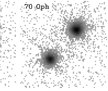
Figure 1: Zeroth-order images of 36 Oph and 70 Oph from Chandra LETG/HRC-S observations. North is up in the figures and in each case the A component is the upper right constituent of the binary. The scale is about $0.14^{\prime\prime}$ per pixel.

Before showing the spectra, it is useful to consider first the zeroth order images that are also provided by the LETG/HRC-S observations. Figure 1 shows these images for the 36 Oph and 70 Oph binaries. Chandra is the first X-ray satellite capable of truly resolving these star systems. Prior to Chandra, the best spatial resolution available was from ROSAT’s High Resolution Imager (HRI). ROSAT/HRI observed both 36 Oph and 70 Oph (Schmitt & Liefke, 2004). In each case, an asymmetry in the HRI image has the appropriate orientation to suggest that both stars are contributing to the emission, but it is impossible to say more than that from those data. In contrast, Figure 1 shows how easily Chandra resolves the binaries. For 36 Oph, we measure a separation of $5.132\pm 0.007^{\prime\prime}$ and a position angle of $141.01\pm 0.12^{\circ}$, while for 70 Oph these quantities are $4.708\pm 0.005^{\prime\prime}$ and $137.75\pm 0.09^{\circ}$, respectively. The stellar separation shown in Figure 1 is also indicative of the separation of the spectra at short wavelengths, though as mentioned in §2 the spatial resolution deteriorates at long wavelengths. For both binaries, the A component is slightly brighter, with 36 Oph A and 70 Oph A accounting for 58.2% and 60.4% of the total X-ray flux, respectively.

The zeroth order images also provide light curves for our targets, which are useful to see whether our spectra are affected by any flaring. The light curves are shown in Figure 2. Some modest, gradual variability with timescales of hours is present for our targets, but the closest thing to a flare is the peak seen for 36 Oph B at $t=31$ ksec, where the flux briefly increases by about a factor of 2. Even if this is a weak flare, it is not strong enough to significantly affect the nature of the spectrum, so no attempt is made to remove it from the data.

4 SPECTRAL ANALYSIS

4.1 Line Identification and Measurement

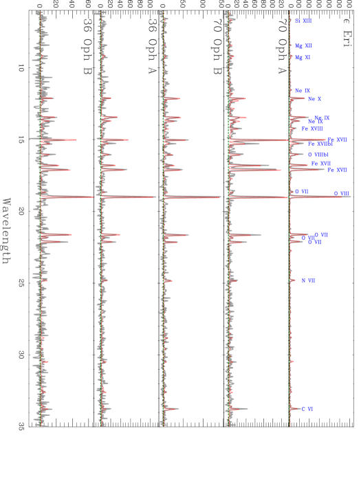
Figure 3: Chandra LETG/HRC-S spectra of 5 moderately active K dwarfs, with line identifications. The spectra have been rebinned by a factor of 3 to improve S/N. For $\lambda>35$ Å, the spectra are also smoothed for the sake of appearance. Red lines are synthetic spectra produced from derived emission measure distributions and coronal abundances (see §4.4), and green lines indicate the contributions of higher orders ($2-5$) to the model spectra.

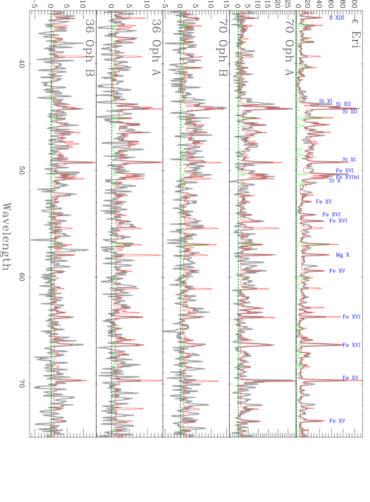
Figure 3: (continued)

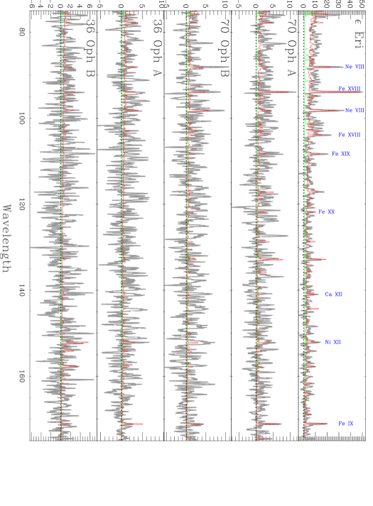
Figure 3: (continued)

The final processed spectra of our five K dwarf stars are shown in Figure 3. The spectra are rebinned by a factor of 3 to improve signal-to-noise (S/N). We use version 4.2 of the CHIANTI atomic database to identify emission lines (Dere et al., 1997; Young et al., 2003). The identified lines are shown in Figure 3 and listed in Table 3. Table 3 lists counts for the detected lines, which are measured by direct integration from the spectra. Line formation temperatures are quoted in the third column of the table, which are based on maxima of contribution functions computed using the ionization equilibrium computations of Arnaud & Rothenflug (1985). Uncertainties quoted in Table 3 are 1$\sigma$. For all undetected lines, we quote 2$\sigma$ upper limits based on summing in quadrature the uncertainties in 5 bins surrounding the location of the line, and then multiplying this sum by 2.

We measure all lines that appear visually to be at least marginally detected. However, all cases in which the uncertainty implies a $<2\sigma$ detection must be considered questionable. After the analysis described in §4.4 is completed, we confirm a posteriori that these questionable detections are at least plausible based on the derived emission measure distributions and abundances (which are constrained primarily by the stronger emission lines in the analysis). Many of the emission lines are blends. We list in Table 3 all lines that we believe contribute a significant (i.e., $\gtrsim 10\%$) amount of flux to the feature based on the line strengths in the CHIANTI database. This determination is reassessed after emission measure distributions are estimated, and model spectra can be computed from them and compared with the data (see §4.4 and Fig. 3). A few of the features identified in Figure 3 are blends of lines of different species (see Table 3). Although we measure counts for these blends and list them in Table 3, these measurements are not used in any of the following analysis.

4.2 Coronal Densities

One coronal property that can in principle be inferred from high-resolution X-ray spectra is the density. The best density diagnostics available in our spectra are various He-like triplets: Si XIII $\lambda$6.7, Mg XI $\lambda$9.2, Ne IX $\lambda$13.6, and O VII $\lambda$21.8. In order of increasing wavelength, these triplets each consist of a resonance line, an intersystem line, and a forbidden line. The ratio of the intersystem and forbidden lines is density sensitive.

Unfortunately, the S/N of the Si XIII, Mg XI, and Ne IX triplets in our spectra is generally not sufficient to allow for a precise density measurement. Due to blending, we simply list in Table 3 the total flux from the Si XIII and Mg XI triplets, and for Ne IX there is no attempt to separate the fluxes of the resonance and intersystem lines. For $\epsilon$ Eri, there is sufficient S/N to separate these lines using profile-fitting techniques and careful correction for blends (e.g., numerous Fe XIX blends for the Ne IX triplet). Ness et al. (2002) have already performed this analysis for $\epsilon$ Eri, so we do not repeat it here.

Since the O VII triplet is the only case where the lines are sufficiently separated and observed with reasonable S/N for all of our stars, we focus our attention on these lines. Line ratios of $f/i\equiv\lambda 22.101/\lambda 21.807$ are computed from the fluxes in Table 3, and we then use the same prescription as Ness et al. (2002) to convert these ratios to electron densities (in cm^-3), which utilizes the results of collisional equilibrium models from Porquet et al. (2001). The resulting densities are listed in Table 4. For 36 Oph B and the two 70 Oph stars, the line ratios are consistent with the low density limit of the diagnostic, so we can only quote upper limits for $n_{e}$. We note that our $\epsilon$ Eri measurement is consistent with the $\log n_{e}=10.03\pm 0.23$ result from Ness et al. (2002) based on these same O VII lines. A solar coronal density derived from these same O VII lines, $\log n_{e}=9.4$, is also listed in Table 4 for the sake of comparison. This value is based on the average $f/i$ ratios observed from a collection of rocket measurements of various active regions (McKenzie, 1987). With the possible exception of 36 Oph A, the coronal densities of our moderately active K dwarfs are not clearly different from the solar value.

All five spectra are basically consistent with a coronal density of $\log n_{e}\approx 10.0$. There is some suggestion that 36 Oph A might have a slightly higher density. The smaller $f/i$ ratio for 36 Oph A is apparent in Figure 3. However, the uncertainty in this ratio is too large to clearly demonstrate higher densities, and the error bar of the $\log n_{e}=10.55\pm 0.51$ measurement for 36 Oph A overlaps the values or upper limits quoted for the other stars. Thus, we conclude that there is no convincing evidence that the coronal densities of our five stars are different.

4.3 Flux Ratios

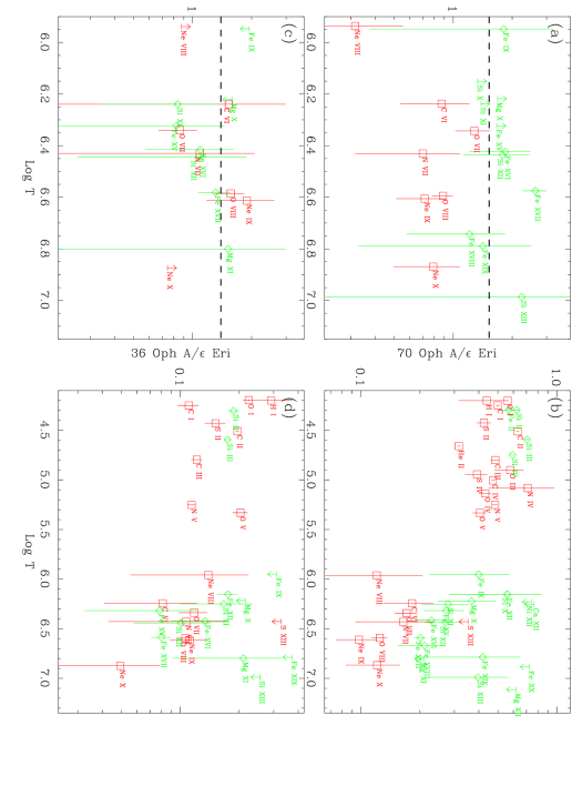
Figure 4: Comparisons of emission line fluxes for various pairs of stars, illustrated by plotting flux ratios as a function of line formation temperature, with red and green data points indicating high-FIP and low-FIP elements, respectively. Dashed lines in panels (a) and (c) indicate the flux ratios of zeroth-order Chandra LETG/HRC-S images.

In §4.4, we compute absolute abundances and emission measure distributions. However, since our primary science goals are comparative in nature (see §1), we can learn a lot by simply comparing the observed line fluxes of our stars with each other without going through the more complex analysis of §4.4. Thus, in Figure 4 we compare the line fluxes of various pairs of stars by plotting line flux ratios versus line formation temperatures, using different symbols and colors to indicate high-FIP (${\rm FIP}>10$ eV) and low-FIP (${\rm FIP}<10$ eV) elements. In cases where there is more than one line of a given species, we simply add fluxes of all lines detected for both stars before computing the flux ratio.

In order to expand the temperature regime explored in this analysis, we have supplemented our Chandra line measurements with UV measurements from spectra taken by the Hubble Space Telescope (HST). These observations, which utilize the Space Telescope Imaging Spectrometer (STIS) instrument on HST, are available for $\epsilon$ Eri, 70 Oph A, and 36 Oph A. The STIS observations of $\epsilon$ Eri and 70 Oph A use the E140M grating, covering a wavelength range of $1150-1730$ Å at a spectral resolution of $R\approx 45,000$, while the available 36 Oph A spectrum uses the E140H grating, covering a wavelength range of $1160-1357$ Å at a higher resolution of $R\approx 110,000$. The UV line measurements are listed in Table 5 along with line formation temperatures from Arnaud & Rothenflug (1985).

All but one of the HST lines are formed either in the chromosphere ($3.8<\log T<4.3$) or transition region ($4.3<\log T<5.8$), but there is one coronal line (with $\log T>5.8$), the Fe XII line at 1242.01 Å. The $\epsilon$ Eri and 70 Oph A fluxes for this line are taken directly from Ayres et al. (2003). Most of the fluxes in Table 5 are our own measurements of the archival HST spectra based on direct flux integration of the lines, with the following exceptions. Most of the $\epsilon$ Eri fluxes are taken from Sim & Jordan (2005), and the fluxes of the H I Lyman-$\alpha$ line at 1215.671 Å are taken from Wood et al. (2005b), who have corrected for interstellar absorption.

The flux ratio plots in Figure 4 illustrate many interesting similarities and differences in the spectra of our K dwarfs. Panel (c) compares fluxes of the two 36 Oph stars. The flux ratios are generally consistent with the flux ratio seen in the zeroth-order Chandra image of the binary (see §3), with one notable exception. For the O VII lines, the 36 Oph A/36 Oph B ratio is lower than one would expect. This is also suggested by the noticeably different O VIII/O VII ratios for these 2 stars apparent in Figure 3. This may be indicative of small differences in the coronal emission measure distributions, with 36 Oph A having a slightly hotter corona.

Much more dramatic differences are seen in Figure 4a, which compares the line fluxes of the two 70 Oph stars. The 70 Oph A/70 Oph B ratios are higher for the low-FIP lines than the high-FIP lines, the implication being that 70 Oph A’s corona apparently has a much more prominent FIP effect than its companion star. The spectral differences between the two stars that lead to this result are readily apparent in Figure 3. (Compare, for example, the relative strengths of the Fe XVII and O VIII lines.) This substantial difference in coronal FIP effect is very surprising considering just how similar the two 70 Oph stars are. Since they are members of the same star system, they clearly have the same age, and these stars also have very similar spectral types, rotation rates, and X-ray surface fluxes (see Table 1). Why do these coronae then exhibit different levels of FIP bias? We will return to this issue in §5.1.

Figure 4b indicates that 70 Oph A not only has a stronger FIP bias than 70 Oph B, but also clearly has a stronger FIP effect than $\epsilon$ Eri, at least in the corona. A relative lack of available low-FIP lines at lower temperatures means that it is not entirely clear whether this difference also exists at transition region temperatures, but the effect certainly seems to be stronger in the corona. The origin of the FIP effect is generally assumed to lie in the chromosphere, where the low-FIP elements are ionized but the high-FIP elements are not. Thus, one would naively expect the FIP effect to be just as apparent in the transition region as it is in the corona. But Figure 4b suggests that the relative strength of a FIP effect can be different between the corona and transition region. This is consistent with solar observations, which show a curious absence of a FIP effect in the transition region (Laming et al., 1995). Perhaps this difference is symptomatic of the transition region emission arising in large part from different magnetic structures than the coronal emission, a conclusion supported by images of the Sun’s corona and transition region, which have very different appearances (Feldman & Laming, 1994).

For both 70 Oph A and 36 Oph A, line ratios with $\epsilon$ Eri are generally lower in the corona than in the transition region (see Figs. 4b and 4d). This is consistent with a higher degree of coronal heating for $\epsilon$ Eri, which is perhaps not surprising since $\epsilon$ Eri is a faster rotator and is slightly more active than 70 Oph A and 36 Oph A (see Table 1).

4.4 Emission Measure and Abundance Analysis

For a more quantitative assessment of the abundances and temperatures of the coronal plasma responsible for the X-ray emission, we perform an emission measure analysis for our five stars based on the line measurements listed in Table 3. This analysis requires assumptions of collisional ionization equilibrium, Maxwellian velocity distributions, and uniform abundances throughout the corona. The emission measure distribution (in units of cm^-3) is defined as

$$EM(T)\equiv n_{e}^{2}\frac{dV}{d\log T},$$ (1)

where dV is a coronal volume element. The observed flux for a given line can then be expressed as

$$f=\frac{1}{4\pi d^{2}}\int G(T,n_{e})EM(T)d\log T,$$ (2)

where $d$ is the stellar distance and $G(T,n_{e})$ is the line contribution function, which includes both the line emissivity and the assumed elemental abundance of the atomic species in question.

Computing a line flux from a known emission measure distribution and with a known elemental abundance is trivial using equation (2). However, the inverse problem of inferring EM(T) and elemental abundances from a set of observed line fluxes in a self-consistent manner is challenging, and a single, unique solution is not strictly obtainable. We use version 2.1 of the PINTofALE software developed by Kashyap & Drake (2000) to perform these calculations, which tackles the inverse problem using a Markov Chain Monte Carlo approach (Kashyap & Drake, 1998).

Before using the measured line counts in Table 3 in the emission measure analysis, we must divide them by the exposure times in Table 2, and we must also correct for interstellar absorption. Interstellar H I column densities are listed in Table 1 for all of our targets. These columns are measured from H I Lyman-$\alpha$ absorption (Wood et al., 2005b). The column densities are converted to wavelength dependent transmittance curves using the prescription of Morrison & McCammon (1983), which provide the necessary information to correct line fluxes for ISM absorption.

Finally, wavelength-dependent effective area curves must be derived for our spectra. The spacecraft dithering that is done during every Chandra observation to smooth detector nonuniformities results in slightly different effective areas from one observation to the next; the exact dithering pattern yields a different aspect solution for converting detector coordinates to spatial coordinates. Deviance from the standard effective area curve is especially noticeable near the two gaps in the HRC-S detector (at $\sim 53$ Å for the minus order spectrum and $\sim 63$ Å for the plus order spectrum), because their exact wavelengths depend on the source position as well as on the aspect solution. Thus, effective area curves must be computed separately for each of our sources, which we do using the appropriate CIAO routines. Since the lines listed in Table 3 are all first order lines, we only have to compute first order effective area curves for the emission measure analysis. However, we also compute effective areas for orders 2–5 to assist in the computation of the synthetic spectra shown in Figure 3 (see below).

All lines listed in Table 3 are considered in the emission measure analysis, with a few exceptions. Blends of lines of different species are not considered. In cases of blends of lines of the same species, we use the predicted line strengths from CHIANTI to divide the flux among the blended lines. The density sensitive lines of the He-like triplets are not included (see §4.2). The PINTofALE software allows for consideration of upper limits, so the 2$\sigma$ upper limits listed in Table 3 are taken into account in the analysis. To improve constraints on the emission measure distributions, we also include the Fe XII $\lambda$1242 line from the HST spectra (see Table 5). The HST and Chandra data are not simultaneous, so variability is potentially a problem for the Fe XII measurements. However, the Fe XII data points in Figures 4b and 4d are basically consistent with the Chandra data points, so we do not believe this is a major issue.

The CHIANTI database is the source of our line emissivities (Dere et al., 1997; Young et al., 2003). We assume a density of $\log n_{e}=10$, which is consistent with the measurements in §4.2 for all of our stars. Temperature-dependent ionization fractions are taken from Mazzotta et al. (1998) based on their collisional equilibrium calculations. The solar photospheric abundances of Grevesse & Sauval (1998) are used for our initial assumed abundances. For elements with detected lines we can compute abundances during the course of the emission measure analysis. However, line measurements alone only allow relative abundances to be computed, meaning the derived emission measure distribution cannot be normalized to an absolute value (though the shape of the distribution can be established). Thus, in the initial emission measure computation the Fe abundance is fixed at the solar photospheric value, and other abundances are measured relative to that. In order to determine the absolute Fe abundance and thereby properly normalize the emission measure distribution, the line-to-continuum ratio must be assessed, a process that will be described below.

Figure 5 shows the emission measure distributions derived by the PINTofALE software using 0.1 dex increments in $\log T$. The derived abundances relative to Fe are listed in Table 4. The emission measure uncertainties shown in Figure 5 and the abundance uncertainties quoted in Table 4 are 90% confidence intervals.

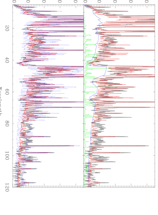
Figure 6: An illustration of how the line-to-continuum ratio is used to derive the absolute coronal Fe abundance, using $\epsilon$ Eri as an example. The bottom panel compares the highly smoothed stellar spectrum with a synthetic spectrum (red line) computed from the emission measure distribution in Fig. 5, assuming a best-fit absolute Fe abundance of ${\rm[Fe/H]}=0.7{\rm[Fe/H]}_{\odot}$. Dotted blue lines show the effect of raising or lowering this value by a factor of 2, where the higher line corresponds to lower [Fe/H]. The upper panel shows the same fit, and also shows explicitly the continuum (blue line) and higher order (green line) contributions to the total line-plus-continuum model spectrum (red line).

As mentioned above, the only way to determine absolute Fe abundances, Fe/H, and thereby properly normalize the emission measure distributions is to assess the relative strengths of the line and continuum emission. Figure 6 shows how this is done, using the $\epsilon$ Eri spectrum as an example. The bottom panel shows a smoothed version of the $\epsilon$ Eri spectrum, and several model spectra computed assuming different values for Fe/H. Higher Fe/H values correspond to lower emission measures, so higher Fe/H leads to a lower continuum. In deciding what Fe/H value leads to the best fit, we believe it is better for the model spectrum to underestimate the observed fluxes than to overestimate it, since missing lines in the atomic database could potentially explain an underestimate. With this in mind, we decide that ${\rm[Fe/H]}=0.7{\rm[Fe/H]}_{\odot}$ leads to a best fit to the data, which is shown in Figure 6. This result and values measured for the other stars are listed in Table 4.

The upper panel of Figure 6 shows the same best fit as in the bottom panel, but explicitly shows the contribution of the continuum to the total flux of the model spectrum, and also shows the contributions of higher orders 2–5 to the total model spectrum, illustrating that these higher orders can contribute a significant amount of flux at certain wavelengths. The best-fit model spectra for all of our stars are shown in Figure 3, assuming our best estimates for Fe/H. The emission measure distributions shown in Figure 5 are normalized based on these absolute abundance determinations.

The EM(T) curves of the five K dwarfs are very similar, both in their shape and in their magnitude, emphasizing once again the similarity of these stars and their coronae. All show a dramatic increase in emission measure from $\log T=5.9$ to $\log T=6.1$. The existence of this “cliff” relies entirely on measurements (or upper limits) of the Fe IX $\lambda$171 line and a few Ne VIII lines (see Table 3), which are the only lines formed at temperatures low enough to constrain EM(T) below $\log T=6.0$. All the EM(T) curves in Figure 5 also have peaks near $\log T=6.5-6.6$, while at higher temperatures the emission measures decrease. Based on these results, we conclude that there is no evidence from these data that the coronae of the five K dwarfs have any substantial differences in temperature distribution, though small variations are present, as suggested by the different O VIII/O VII ratios for 36 Oph A and B, for example.

The only clear signature of coronal differences among these stars is from the abundance measurements. In Figure 7, the coronal abundances listed in Table 4 are plotted relative to the stellar photospheric abundances listed in Table 1. Note that these photospheric abundances, which are quoted relative to solar abundances, are measured by direct line-by-line comparison of solar and stellar absorption lines, meaning that the abundances are truly relative abundances that do not assume any absolute abundance measurements for the Sun or the stars (Allende Prieto et al., 2004). We use the Grevesse & Sauval (1998) solar photospheric abundances listed in Table 4 to convert the relative abundances in Table 1 to absolute reference photospheric abundances, for use in the creation of Figure 7. There are no photospheric abundances for 36 Oph B or 70 Oph B (see Table 1), so we simply assume that these stars have abundances identical to their companion stars, 36 Oph A and 70 Oph A, respectively. Also, there are no stellar measurements of N, Ne, or S abundances for any of the stars, so we simply assume that the relative O abundances quoted in Table 1 apply to these other 3 elements.

The abundances in Figure 7 are plotted versus FIP, where a dotted line is used to divide the elements into low-FIP and high-FIP regimes. A few of the stars seem to show some evidence for a solar-like FIP effect (e.g., 70 Oph A, 36 Oph AB), with the low-FIP elements being higher in abundance relative to the high-FIP elements. However, neon seems to be discrepant, with higher abundances than the other high-FIP elements. Another curious aspect of these measurements is that even for those stars that show the solar-like FIP bias (i.e., high low-FIP abundances), the measurements are different from the standard solar-like FIP bias in that they seem to be more consistent with the high-FIP elements being depleted in the corona rather than the low-FIP elements being enhanced.

The apparent lack of any evident low-FIP abundance enhancements in the corona for any of our stars originates from our measurements of the absolute Fe/H abundances using the line-to-continuum ratios (see Fig. 6). These Fe/H measurements range from ${\rm[Fe/H]}=0.68-1.57{\rm[Fe/H]_{*}}$, where ${\rm[Fe/H]_{*}}$ is the reference photospheric abundance. Only 70 Oph A actually has a ratio above the stellar photospheric value (see Fig. 7). Similar Fe/H values are measured by Telleschi et al. (2005) from XMM spectra of six solar-like G stars, and many of these stars show evidence for high-FIP depletions in the corona similar to those seen for 70 Oph A and 36 Oph AB in Figure 7. Some analyses of solar flare X-ray spectra have also found similar abundance patterns (Fludra & Schmelz, 1995). These results seem to suggest that stellar fractionation processes are capable of both depleting high-FIP elements and enhancing low-FIP elements, depending on the circumstances. These issues will be discussed more in §5.2.

Figure 8 puts the abundances from Figure 7 into the same plot for all five stars, normalized to the Fe abundance. Dotted lines connect the high-FIP elements in the figure, indicating the high-FIP abundance relative to Fe. The different levels of FIP bias noted on the basis of the line flux ratios (see §4.3) are here apparent from the actual abundance measurements, with Figure 8 suggesting the following sequence of increasing FIP effect: 70 Oph B, $\epsilon$ Eri, 36 Oph A, 36 Oph B, 70 Oph A. As noted in §4.3, it is remarkable that the two 70 Oph stars are on opposite ends of this sequence, with 70 Oph A having a much stronger FIP effect than 70 Oph B despite the similarities between these stars in almost all other respects. Although the overall level of FIP bias is different for the five stars, Figure 8 suggests similar relative abundances for the high-FIP elements for all five stars, with O being low, Ne being high, and C and N being generally somewhere in between.

Confidence in a true commonality for this high-FIP abundance pattern suffers from the size of the error bars in the abundance measurements, particularly for C and N (see Fig. 7), but high Ne/O ratios have been found to exist for many stellar coronae (Drake & Testa, 2005). We list Ne/O ratios for our stars in Table 4. These ratios are all about a factor of 2 larger than the solar value of ${\rm Ne/O}=0.18$ (Grevesse & Sauval, 1998; Schmelz et al., 2005; Young, 2005). The average and standard deviation of the K dwarf Ne/O ratios are ${\rm Ne/O}=0.37\pm 0.04$, which agrees well with the average value of ${\rm Ne/O}=0.41$ derived by Drake & Testa (2005) from a much larger sample of stars. The Drake & Testa (2005) sample consists almost entirely of very active stars. That our sample yields similar results demonstrates that the high coronal Ne/O ratios extend to less active stars, though it must be emphasized that our sample of K dwarfs are still significantly more active than the comparatively inactive Sun. Coronal abundance measurements for stars as inactive as the Sun are difficult, since their faintness in X-rays makes it difficult to obtain X-ray spectra with sufficient S/N to measure precise abundances.

5 DISCUSSION

5.1 The 70 Oph Abundance Discrepancy

Perhaps the most interesting result of our analysis is the coronal abundance difference between the two members of the 70 Oph binary, which is unexpected since these two stars are so similar in all other respects. Previous stellar observations have shown that the traditional solar-like FIP effect is generally observed for stars of low to moderate activity (Laming et al., 1996; Drake et al., 1997; Laming & Drake, 1999). In contrast, for very active stars an inverse FIP effect is generally observed, where low-FIP elements have coronal abundances that are lower relative to photospheric values than is the case for high-FIP elements (Brinkman et al., 2001; Drake et al., 2001; Güdel et al., 2001; Huenemoerder et al., 2001; Sanz-Forcada et al., 2003) Coronae of stars of intermediate activity are generally found to have abundances with little or no dependence on FIP (Drake et al., 1995; Audard et al., 2001; Ball et al., 2005). Thus, the general picture is of the FIP effect being dependent on activity, with the low-FIP element abundances decreasing in the corona with increasing activity (Audard et al., 2003; Telleschi et al., 2005).

However, if two stars as similar as 70 Oph A and B can have drastically different levels of FIP bias, this makes it very difficult for any simple paradigm to explain why different stars have different coronal abundance patterns. One potential way out of this dilemma is to appeal to time dependent effects to explain the curious 70 Oph results. Time variations in FIP bias are observed in solar active regions, which emerge with nearly photospheric abundances and then acquire a FIP bias that increases on a timescale of days (Widing & Feldman, 2001). Perhaps at the time of our Chandra observation of 70 Oph, the visible part of 70 Oph B’s corona was dominated by young active regions while the visible part of 70 Oph A’s corona was dominated by old active regions, in which case the observed difference in FIP behavior is temporary. The only way to test this hypothesis would be to reobserve 70 Oph, preferably several times. Sanz-Forcada et al. (2003) looked for abundance variations in multiple observations of the very active K dwarf AB Dor, with the observations encompassing a range of activity levels for the star. However, no abundance variability was found.

5.2 Depletions of High-FIP Elements in Stellar Coronae

Another puzzling result to arise from our coronal abundance analysis is the apparent depletion of high-FIP elements in the corona with respect to the photosphere, at least for a few of our stars. Although the origin of the FIP effect and inverse FIP effect is not well understood, the cause is thought to lie in the chromosphere, where the low-FIP elements are ionized and therefore subject to forces that the neutral high-FIP elements are not subject to. The general assumption is that these forces, whatever their nature, preferentially act on low-FIP elements, which leads to these elements having nonphotospheric abundances in the corona. For the Sun and relatively inactive stars, the low-FIP coronal abundance trend is towards high abundances, while for very active stars the trend is towards low abundances.

In this simple scenario, the elements with the highest FIP should always have coronal abundances closest to the photospheric values since they are less subject to whatever forces are causing the FIP effect. This, however, is not consistent with what we see in our data. For example, for every single one of our stars the coronal O abundance is farther from the photospheric abundance than the Fe and Si abundances, with the data suggesting a depletion of O in the corona in every case. Note that measured photospheric O, Si, and Fe abundances exist for our stars and are taken into account in the analysis (see Table 1), so a lack of photospheric reference abundances is not an issue here, though it is often a problem in interpreting the coronal abundance measurements for very active stars (see, e.g., Sanz-Forcada et al., 2004). Telleschi et al. (2005) find similar evidence for high-FIP element depletions for many of the active solar-like stars in their sample. Other examples of coronal abundance patterns that are also difficult for any simple FIP-based fractionation model to explain are reported by Brinkman et al. (2001), Drake et al. (2001), Huenemoerder et al. (2003), and Sanz-Forcada et al. (2004).

Another observational result that the simple FIP-dependent scenarios cannot easily explain is that the Ne/O ratios of many different stars are the same, regardless of whether the stars generally show a solar-like FIP effect, no FIP effect, or an inverse FIP effect. All of our stars and all of those in the larger sample of Drake & Testa (2005) suggest ${\rm Ne/O}\approx 0.4$. Either the processes that cause the observed coronal abundance anomales are not dependent on FIP in any simple, monotonic fashion, or there are other fractionation forces at work that have nothing to do with FIP whatsoever.

Some solar flare observations have also suggested abundance patterns similar to that seen for 70 Oph A in Figure 8, with high-FIP elements being depleted in the corona (Veck & Parkinson, 1991; Fludra & Schmelz, 1995). The Ne/O ratios observed from solar active regions also show substantial variation about the mean solar value of 0.18, demonstrating a deviation from the average FIP effect even in relatively quiescent plasma (Schmelz et al., 1996). It has been proposed that photoionization by coronal X-rays can lead to nonequilibrium ionization conditions in the atmospheric regions where fractionation is taking place (Shemi, 1991). Since Ne, for example, has a higher photoionization cross section than O, Ne could be photionized while O remains neutral despite Ne having a higher FIP. Analogous effects have been proposed to explain a factor of 2 depletion of He in the solar wind (von Steiger & Geiss, 1989; von Steiger et al., 2000).

For active stars, the irradiation of stellar atmospheres by coronal X-rays would be more intense, potentially making such photoionization effects more important. This could perhaps explain the high Ne/O ratios seen for active stars, but it does not obviously explain other aspects of the observed abundance patterns, such as why high-FIP elements can be depleted in stellar coronae. Clearly, we are still far from understanding the fractionation forces operating in stellar atmospheres, and far from understanding why they appear to operate so differently on different stars.

5.3 The Ne/O Controversy

The whole issue of Ne/O ratios deserves additional comment since solar/stellar Ne and O abundances have recently become controversial topics. The discord began when complex 3D hydrodynamic models of the solar atmosphere were used to reassess solar abundances, and it was then claimed that the abundances of many light elements such as C, N, and O needed to be revised downward by $25-35$% (Allende Prieto et al., 2001, 2002; Asplund et al., 2005). Unfortunately, these suggested changes seriously damage the remarkably good agreement that exists between models of the solar interior and various helioseismological measurements, when older abundances are used (Basu & Antia, 2004; Bahcall et al., 2005a).

It has been noted that these problems can be mitigated by increasing the assumed solar Ne abundance by a factor of 2–3 (Antia & Basu, 2005; Bahcall et al., 2005b). The reason why such an increase can be reasonably proposed is that the solar Ne abundance is poorly known. There are no spectroscopic diagnostics of Ne in the photosphere, which means that the solar Ne abundance must be inferred from coronal or transition region measurements. But this is dangerous given the existence of fractionation processes that result in differences between coronal and photospheric abundances (see §5.2).

When Drake & Testa (2005) demonstrated that stellar Ne/O ratios have values consistent with ${\rm Ne/O}=0.41$, which is significantly higher than the ratio assumed for the Sun (${\rm Ne/O}=0.18$), they proposed that the stellar measurements represent a better estimate of the solar/stellar photospheric Ne/O ratios than the lower solar ratio. Not only would this explain the remarkably consistent stellar Ne/O ratios, but it would also solve the discrepancies between solar interior models and helioseismology induced by the revised C, N, and O abundances. Unfortunately, very recent reassessments of the solar coronal Ne/O ratio based on both full-disk and spatially resolved data seem to confirm that the solar Ne/O ratio is truly a factor of 2 lower than those observed from the stars in the Drake & Testa (2005) sample, which are more active than the Sun (Young, 2005; Schmelz et al., 2005). Thus, the evidence at present seems to suggest that the Sun really does have a different coronal Ne/O ratio than active stars.

Furthermore, there are measurements of Ne/O for stars as inactive as the Sun that suggest low, solar-like ratios. These measurements generally carry large uncertainties because the Ne IX and Ne X lines used to provide Ne abundances are generally weak for the cooler coronae of inactive stars. Nevertheless, Raassen et al. (2002) quote a value of ${\rm Ne/O}=0.21$ for Procyon, though Sanz-Forcada et al. (2004) find a higher value of ${\rm Ne/O}=0.40$. Raassen et al. (2003) report ${\rm Ne/O}=0.18$ and ${\rm Ne/O}=0.24$ for $\alpha$ Cen A and B, respectively, and Telleschi et al. (2005) find ${\rm Ne/O}\approx 0.14$ for $\beta$ Com, though with large uncertainties. A compilation of measurements in Güdel (2004), including those mentioned above, provides some evidence for a weak correlation of Ne/O with activity.

As mentioned in §4.4, the high Ne/O ratios seen for our K dwarfs are significant because they demonstrate that the high Ne/O ratio found by Drake & Testa (2005) applies to stars less active than most of those in their sample. But our K dwarfs are still significantly more active than the Sun. There are two possible explanations for the different Ne/O ratios that exist for the Sun and more active stars: (a) The stellar Ne/O measurements are representative of the true cosmic abundance and the low solar Ne/O measurements are a product of some fractionation mechanism operating in the solar atmosphere but not the active stars, or (b) The solar Ne/O measurement is characteristic of the true cosmic abundance and the high stellar ratios are due to a fractionation mechanism that is not present for the Sun. At first glance, the latter interpretation seems more likely, partly because the low solar Ne/O abundances are known to exist down to at least transition region temperatures (Young, 2005), and partly because it is easier to imagine active stars having strong fractionation effects that result in substantial differences between coronal and photospheric Ne/O ratios. However, this would leave the solar interior problems unresolved.

Without direct photospheric measurements of Ne, it is not possible to say much about solar/stellar Ne abundances with any great amount of confidence. Perhaps for Ne it is best to measure the cosmic abundance from a very different astronomical source. We note that Gloeckler & Geiss (2004) have estimated O and Ne abundances in the local ISM using Ulysses and ACE measurements of pickup ions within our solar system, and they find ${\rm Ne/O}\approx 0.41$. This is in better agreement with the active star ratio than the solar ratio, though it must be noted that the ISM measurements come with their own set of systematic uncertainties and assumptions regarding dust depletion, deflection at the heliopause, and ISM ionization fraction.

5.4 Do Winds Correlate with Coronal FIP Bias?

A major motivation behind our Chandra observations was to see whether coronal differences in our K dwarf sample could be correlated with observed differences in the strengths of their winds. However, the only coronal properties that clearly vary in this sample of stars are the abundances. The overall coronal activity levels of these stars are about the same, and the Chandra data cannot distinguish any significant density or temperature differences in the stellar coronae.

Can the observed abundance variations be correlated with wind strength? The mass loss rates per unit surface area of 36 Oph, $\epsilon$ Eri, and 70 Oph (in solar units) are 18.1, 49.3, and 85.7, respectively (see Table 1). (Unfortunately, we only know the combined mass loss rates for the 36 Oph and 70 Oph binaries and not the contributions of the individual stars.) The 36 Oph binary has the weakest wind, and both stars have coronae that show a modest FIP effect (see Fig. 8). This suggests a potential connection between weak winds and strong FIP bias. The stronger wind and weak-or-no FIP effect of $\epsilon$ Eri would support such a connection, but the fact that 70 Oph consists of both a high FIP-bias star (70 Oph A) and a no-or-inverse FIP-bias star (70 Oph B) complicates the interpretation of its high mass loss measurement. If the FIP-bias/wind anticorrelation suggested by 36 Oph and $\epsilon$ Eri is true, that would imply that 70 Oph B must be responsible for most of 70 Oph’s strong wind. Small number statistics preclude any definitive conclusions on the nature of any FIP/wind connection, but we note that for the Sun different levels of FIP bias are seen for low and high speed streams (von Steiger et al., 2000). This suggests that a FIP/wind connection of some sort is not implausible, but it must be noted that our X-ray spectra will be characteristic of brighter, high density plasma still confined in coronal loops rather than outflowing wind material, so any FIP/wind connection would have to be indirect.

6 SUMMARY

We have analyzed Chandra LETG/HRC-S spectra of five very similar moderately active K dwarf stars (36 Oph AB, 70 Oph AB, and $\epsilon$ Eri), measuring emission measure distributions and coronal abundances from the spectra for all five stars. Our results are summarized as follows:

1.

Our observations of 36 Oph and 70 Oph have resolved these binaries in X-rays for the first time, showing that 36 Oph A and 70 Oph A account for 58.2% and 60.4% of the binaries’ X-ray emission, respectively.

2.

We estimate coronal densities from the flux ratios of the O VII $\lambda$21.8 triplet lines. All five stars have densities consistent with $\log n_{e}\approx 10.0$.

3.

The emission measure distributions of our five K dwarfs are very similar, so there is no evidence for significant coronal temperature variations among these stars.

4.

Elemental abundances are the only coronal properties that clearly are different within our sample of moderately active K dwarfs. The two extremes are 70 Oph A, which shows a prominent solar-like FIP effect, and 70 Oph B, which has no FIP bias at all or possibly even a weak inverse FIP effect. The strong abundance difference between 70 Oph A and 70 Oph B is very surprising, considering how similar these two stars are in almost every other respect. This will be very difficult for any simple model of the FIP effect to explain, though we cannot rule out the possibility that the apparent 70 Oph AB discrepancy could be a temporary product of coronal abundance variability, such as that seen during the evolution of solar active regions.

5.

For our stars, high-FIP elements generally seem to be depleted in the corona relative to the photosphere, which is very different from the standard picture of the solar FIP effect, with low-FIP elements enhanced in the corona and high-FIP elements unchanged from photospheric abundances. It is very unlikely that any simple fractionation model based on FIP as the sole discriminant is likely to explain the variety of abundance patterns that have been observed in stellar coronae.

6.

The Ne/O ratio is essentially the same for our five stars, ${\rm Ne/O}=0.37\pm 0.04$. This value is a factor of 2 higher than the solar value but it agrees very well with the measurement of ${\rm Ne/O}=0.41$ from Drake & Testa (2005) based on a large selection of stars. Our stellar sample is generally less active than the Drake & Testa (2005) sample, so our measurements demonstrate that high stellar Ne/O coronal abundance ratios extend to lower activity levels.

7.

A small sample size precludes any definitive conclusions about whether the coronal abundance variations we see in our data are connected in any way with variations that also exist in measured mass loss rates for these stars. The 36 Oph AB and $\epsilon$ Eri measurements could suggest an anticorrelation between coronal FIP bias and wind strength, which would mean that 70 Oph B would have to be responsible for the particularly strong wind observed from the 70 Oph binary. Unfortunately, this prediction is untestable at the present time.

Table 1: Stellar Information

Property	36 Ophiuchi		70 Ophiuchi		$\epsilon$ Eridani	Refs.
	A	B	A	B
Other Name	HD 155886	HD 155885	HD 165341	HD 165341B	HD 22049
Spect. Type	K1 V	K1 V	K0 V	K5 V	K1 V
Dist. (pc)	5.99	5.99	5.09	5.09	3.22	1
Radius (R⊙)	0.69	0.59	0.85	0.66	0.78	2
Prot (days)	20.3	22.9	19.7	22.9	11.7	3,4
Log Lx	28.10	27.96	28.27	28.09	28.32	5
$\dot{M}$ ($\dot{M}_{\odot}$)	15		100		30	6
$\log N_{H}$	17.85		18.06		17.88	7
$\log{\rm[C/C_{\odot}]}$	$-0.40$	…	$-0.10$	…	$-0.24$	8
$\log{\rm[O/O_{\odot}]}$	$-0.14$	…	$0.03$	…	$-0.04$	8
$\log{\rm[Mg/Mg_{\odot}]}$	$-0.28$	…	$0.09$	…	$-0.03$	8
$\log{\rm[Si/Si_{\odot}]}$	$-0.07$	…	$0.18$	…	$-0.01$	8
$\log{\rm[Ca/Ca_{\odot}]}$	$-0.15$	…	$0.09$	…	$-0.01$	8
$\log{\rm[Fe/Fe_{\odot}]}$	$-0.30$	…	$-0.05$	…	$-0.06$	8
$\log{\rm[Ni/Ni_{\odot}]}$	$-0.20$	…	$0.06$	…	$-0.06$	8

References. — (1) Perryman et al. 1997. (2) Barnes et al. 1978. (3) Donahue et al. 1996. (4) Noyes et al. 1984. (5) Schmitt & Liefke 2004. (6) Wood et al. 2005a. (7) Wood et al. 2005b. (8) Allende Prieto et al. 2004.

Table 2: Chandra LETG/HRC-S Observations

Star	Obs. ID	Date	Start Time	Exp. Time
			(UT)	(ksec)
$\epsilon$ Eri	1869	2001 Mar. 21	7:17:12	105.91
36 Oph	4483	2004 June 1	10:22:33	77.90
70 Oph	4482	2004 July 19	22:59:01	78.94

Table 3: Chandra Line Measurements

Ion	$\lambda_{rest}$	$\log T$	Counts
	(Å)		$\epsilon$ Eri	70 Oph A	70 Oph B	36 Oph A	36 Oph B
Si XIII	6.648	6.99	$127.1\pm 22.4$	$50.3\pm 19.8$	$22.5\pm 18.8$	$<32.4$	$<32.0$
Si XIII	6.688	6.99
Si XIII	6.740	6.99
Mg XII	8.419	7.11	$51.9\pm 15.7$	$<32.0$	$<32.8$	$<32.4$	$<30.8$
Mg XII	8.425	7.11
Mg XI	9.169	6.80	$185.4\pm 29.6$	$<38.8$	$<40.0$	$38.9\pm 21.1$	$25.7\pm 20.4$
Mg XI	9.231	6.80
Mg XI	9.314	6.79
Ne IX	11.547	6.61	$61.8\pm 17.7$	$<34.0$	$<33.0$	$<31.6$	$<32.4$
Ne X	12.132	6.87	$481.8\pm 32.5$	$58.3\pm 17.4$	$73.7\pm 16.3$	$23.8\pm 13.9$	$<32.0$
Ne X	12.138	6.87
Ne IX	13.447	6.58	$818.1\pm 39.8$	$85.6\pm 21.5$	$92.4\pm 18.8$	$94.0\pm 21.9$	$40.7\pm 16.0$
Ne IX	13.553	6.58
Ne IX	13.699	6.58	$367.8\pm 30.4$	$30.2\pm 16.5$	$69.4\pm 17.9$	$38.1\pm 15.9$	$29.2\pm 15.5$
Fe XVIII	14.203	6.74	$205.1\pm 31.4$	$39.4\pm 15.6$	$<33.8$	$<31.6$	$<32.0$
Fe XVIII	14.208	6.74
Fe XVII	15.015	6.59	$1207.1\pm 46.8$	$231.7\pm 24.6$	$83.7\pm 18.3$	$103.2\pm 18.3$	$67.7\pm 18.5$
Fe XVII	15.262	6.59	$709.1\pm 42.3$	$155.9\pm 22.8$	$69.8\pm 19.5$	$61.8\pm 17.0$	$40.9\pm 17.5$
O VIII	15.176	6.65
Fe XIX	15.198	6.83
O VIII	16.006	6.63	$515.5\pm 35.0$	$86.7\pm 20.3$	$64.8\pm 18.9$	$59.6\pm 18.2$	$50.5\pm 17.6$
Fe XVIII	16.005	6.73
Fe XVIII	16.072	6.73
Fe XVII	16.778	6.58	$721.7\pm 35.7$	$165.5\pm 22.4$	$62.9\pm 18.9$	$46.1\pm 14.8$	$52.0\pm 17.9$
Fe XVII	17.053	6.58	$1660.9\pm 50.6$	$325.2\pm 27.5$	$128.4\pm 20.9$	$138.4\pm 22.1$	$100.2\pm 19.5$
Fe XVII	17.098	6.58
O VII	18.627	6.34	$152.9\pm 21.8$	$42.5\pm 17.9$	$<33.6$	$18.1\pm 12.9$	$19.9\pm 15.1$
O VIII	18.967	6.59	$2272.3\pm 55.7$	$283.7\pm 25.2$	$320.0\pm 27.1$	$241.3\pm 23.6$	$154.2\pm 21.7$
O VIII	18.973	6.59
O VII	21.602	6.32	$773.2\pm 35.7$	$128.6\pm 19.2$	$119.4\pm 19.2$	$82.4\pm 17.1$	$96.9\pm 20.1$
O VII	21.807	6.32	$152.8\pm 21.6$	$25.5\pm 13.7$	$15.0\pm 13.5$	$29.2\pm 13.2$	$25.6\pm 13.2$
O VII	22.101	6.31	$504.6\pm 29.9$	$74.7\pm 17.5$	$44.0\pm 14.9$	$56.7\pm 16.3$	$74.5\pm 17.2$
N VII	24.779	6.43	$211.7\pm 26.5$	$34.8\pm 14.3$	$49.8\pm 18.1$	$22.7\pm 13.3$	$20.9\pm 14.5$
N VII	24.785	6.43
C VI	33.734	6.24	$340.5\pm 25.4$	$62.1\pm 17.3$	$71.1\pm 19.1$	$27.7\pm 13.6$	$18.1\pm 14.7$
C VI	33.740	6.24
S XIII	35.667	6.43	$94.1\pm 21.5$	$<33.2$	$<33.2$	$<30.8$	$<32.0$
Si XI	43.763	6.25	$133.2\pm 22.8$	$41.0\pm 15.1$	$<33.0$	$19.6\pm 14.6$	$<30.4$
Si XII	44.019	6.44	$185.2\pm 24.0$	$52.4\pm 17.2$	$34.4\pm 14.3$	$18.8\pm 12.9$	$<31.4$
Si XII	44.165	6.44	$288.0\pm 26.7$	$74.9\pm 17.8$	$37.0\pm 17.3$	$28.9\pm 15.1$	$27.0\pm 14.9$
Si XI	49.222	6.24	$195.8\pm 26.1$	$50.7\pm 16.7$	$<33.2$	$35.2\pm 15.4$	$42.0\pm 17.0$
Fe XVI	50.361	6.43	$246.2\pm 28.0$	$40.0\pm 16.1$	$28.1\pm 16.9$	$<33.8$	$<32.8$
Fe XVI	50.565	6.43	$147.3\pm 23.6$	$53.1\pm 16.8$	$<31.6$	$<31.8$	$<30.8$
Si X	50.524	6.15
Si X	50.691	6.15	$71.7\pm 21.2$	$40.0\pm 15.9$	$<30.0$	$<31.0$	$<31.6$
Fe XV	52.911	6.32	$50.1\pm 16.0$	$<27.2$	$<28.6$	$<26.4$	$<26.0$
Fe XVI	54.127	6.43	$96.7\pm 17.3$	$<28.2$	$<27.8$	$<26.8$	$<27.6$
Fe XVI	54.710	6.43	$121.0\pm 19.4$	$32.8\pm 15.6$	$<32.2$	$<27.8$	$<27.8$
Mg X	57.876	6.22	$144.9\pm 23.2$	$53.2\pm 15.0$	$<31.6$	$<31.2$	$19.7\pm 13.0$
Mg X	57.920	6.22
Fe XV	59.405	6.32	$107.8\pm 20.8$	$30.6\pm 14.5$	$<32.8$	$<31.0$	$<30.2$
Fe XVI	63.711	6.42	$140.6\pm 18.8$	$37.8\pm 12.5$	$19.3\pm 11.5$	$28.7\pm 13.1$	$20.7\pm 12.7$
Fe XVI	66.357	6.42	$363.2\pm 29.1$	$88.7\pm 20.3$	$42.8\pm 17.6$	$38.8\pm 17.5$	$40.9\pm 17.6$
Fe XVI	66.249	6.42
Fe XV	69.682	6.32	$285.2\pm 25.8$	$76.5\pm 17.4$	$<31.4$	$22.3\pm 12.9$	$27.0\pm 13.2$
Fe XV	73.472	6.32	$118.9\pm 20.1$	$<33.6$	$<32.4$	$<29.4$	$<31.4$
Ne VIII	88.082	5.96	$176.0\pm 21.3$	$21.2\pm 14.9$	$67.2\pm 19.2$	$24.5\pm 14.4$	$<28.0$
Ne VIII	88.120	5.96
Fe XVIII	93.923	6.68	$275.7\pm 33.0$	$62.3\pm 20.9$	$51.5\pm 20.5$	$<42.0$	$<42.0$
Ne VIII	98.260	5.94	$153.7\pm 27.3$	$<43.4$	$<42.2$	$<42.0$	$<41.8$
Fe XVIII	103.937	6.68	$108.1\pm 28.9$	$<42.8$	$<42.6$	$<41.6$	$<39.6$
Fe XIX	108.355	6.79	$112.0\pm 30.1$	$46.9\pm 22.6$	$33.1\pm 19.8$	$<41.6$	$<42.6$
Fe XX	121.845	6.88	$55.9\pm 26.7$	$<40.4$	$<41.0$	$<41.4$	$<39.0$
Ca XII	141.038	6.25	$53.7\pm 24.2$	$<41.0$	$<42.0$	$<41.0$	$<41.4$
Ni XII	152.154	6.23	$58.5\pm 24.3$	$<43.4$	$<43.0$	$<42.4$	$<40.4$
Fe IX	171.073	5.95	$114.2\pm 21.3$	$45.6\pm 18.2$	$25.2\pm 17.3$	$<35.4$	$18.2\pm 16.3$

Table 4: Densities and Abundances

	$\epsilon$ Eri	70 Oph A	70 Oph B	36 Oph A	36 Oph B	Sun
$\log n_{e}$	$9.82^{+0.33}_{-0.72}$	$<10.89$	$<12.06$	$10.55\pm 0.51$	$<10.88$	9.4
${\rm Fe/Fe_{\odot}}$	0.7	1.4	0.6	0.5	0.5	1
$\log{\rm[Fe/H]}$	$-4.65$	$-4.35$	$-4.72$	$-4.80$	$-4.80$	$-4.50$
$\log{\rm[C/Fe]}$	$0.80_{-0.06}^{+0.04}$	$0.48_{-0.15}^{+0.16}$	$1.02_{-0.13}^{+0.39}$	$0.53_{-0.35}^{+0.28}$	$0.44_{-0.34}^{+0.44}$	1.02
$\log{\rm[N/Fe]}$	$0.36_{-0.09}^{+0.04}$	$0.14_{-0.36}^{+0.16}$	$0.71_{-0.29}^{+0.25}$	$0.33_{-0.56}^{+0.26}$	$0.21_{-0.55}^{+0.38}$	0.42
$\log{\rm[O/Fe]}$	$1.11_{-0.03}^{+0.02}$	$0.82_{-0.05}^{+0.10}$	$1.33_{-0.07}^{+0.16}$	$1.08_{-0.10}^{+0.16}$	$1.09_{-0.16}^{+0.15}$	1.33
$\log{\rm[Ne/Fe]}$	$0.67_{-0.02}^{+0.04}$	$0.38_{-0.12}^{+0.14}$	$0.94_{-0.11}^{+0.12}$	$0.69_{-0.24}^{+0.14}$	$0.58_{-0.64}^{+0.21}$	0.58
$\log{\rm[Mg/Fe]}$	$0.11_{-0.07}^{+0.07}$	$0.16_{-0.17}^{+0.15}$	…	$0.47_{-1.03}^{+0.10}$	$0.15_{-0.69}^{+0.40}$	0.08
$\log{\rm[Si/Fe]}$	$-0.02_{-0.06}^{+0.06}$	$0.01_{-0.18}^{+0.09}$	$0.19_{-0.48}^{+0.24}$	$0.11_{-0.38}^{+0.13}$	$-0.07_{-0.56}^{+0.36}$	0.05
$\log{\rm[S/Fe]}$	$-0.20_{-0.26}^{+0.14}$	…	…	…	…	$-0.17$
$\log{\rm[Ca/Fe]}$	$-0.65_{-1.01}^{+0.25}$	…	…	…	…	$-1.14$
$\log{\rm[Ni/Fe]}$	$-1.37_{-0.62}^{+0.19}$	…	…	…	…	$-1.25$
${\rm Ne/O}$	0.36	0.36	0.40	0.41	0.31	0.18

Table 5: HST Line Measurements

Ion	$\lambda_{rest}$	$\log T$	Flux ($10^{-15}$ ergs cm-2 s-1)
	(Å)		$\epsilon$ Eri	70 Oph A	36 Oph A
C III	1174.933	4.80	$41.0\pm 6.0$	$22.4\pm 1.7$	$4.2\pm 0.6$
C III	1175.263	4.80	$41.0\pm 6.0$	$15.9\pm 1.7$	$3.6\pm 0.7$
C IIIbl	1175.69	4.80	$149.0\pm 6.0$	$70.5\pm 3.6$	$22.3\pm 1.0$
C III	1175.987	4.80	$41.0\pm 6.0$	$21.0\pm 2.1$	$3.6\pm 0.8$
C III	1176.370	4.80	$46.0\pm 6.0$	$24.6\pm 1.9$	$4.9\pm 0.9$
Si II	1190.416	4.37	$10.0\pm 3.0$	$5.8\pm 0.7$	$2.1\pm 0.4$
Si II	1193.290	4.37	$9.0\pm 4.0$	$4.2\pm 0.6$	$2.0\pm 0.4$
Si II	1194.500	4.37	$18.0\pm 3.0$	$10.6\pm 0.9$	$2.8\pm 0.3$
Si II	1197.394	4.37	$10.0\pm 4.0$	$3.6\pm 0.9$	$1.2\pm 0.3$
Si III	1206.500	4.60	$360.0\pm 10.0$	$257.9\pm 3.9$	$62.8\pm 1.3$
H I	1215.671	4.20	$48800\pm 9760$	$21400\pm 4280$	$14200\pm 2840$
O V	1218.344	5.33	$68.0\pm 4.0$	$28.0\pm 2.0$	$13.8\pm 0.9$
N V	1238.821	5.25	$94.0\pm 3.0$	$45.1\pm 1.2$	$10.7\pm 0.5$
Fe XII	1242.01	6.15	$12.0\pm 0.8$	$6.7\pm 0.5$	$2.1\pm 0.2$
N V	1242.804	5.25	$46.0\pm 2.0$	$22.7\pm 0.7$	$5.3\pm 0.4$
S II	1253.811	4.43	$6.6\pm 0.5$	$3.0\pm 0.3$	$1.3\pm 0.2$
S II	1259.519	4.43	$9.9\pm 0.5$	$4.0\pm 0.4$	$1.2\pm 0.2$
Si II	1260.422	4.35	$19.1\pm 3.0$	$10.0\pm 0.5$	$3.7\pm 0.3$
Si II	1264.738	4.35	$50.5\pm 5.0$	$35.2\pm 0.8$	$9.7\pm 0.4$
Si II	1265.002	4.35	$17.2\pm 3.0$	$9.3\pm 0.6$	$3.1\pm 0.3$
C I	1288.422	4.25	$5.7\pm 0.4$	$2.8\pm 0.2$	$0.8\pm 0.1$
Si III	1294.545	4.59	$5.2\pm 0.5$	$3.4\pm 0.3$	$0.8\pm 0.2$
Si III	1296.726	4.59	$4.1\pm 0.5$	$2.4\pm 0.2$	$0.8\pm 0.2$
Si IIIbl	1298.93	4.59	$16.7\pm 0.5$	$10.3\pm 0.4$	$2.8\pm 0.2$
Si III	1301.149	4.59	$2.8\pm 0.5$	$1.6\pm 0.2$	…
O I	1302.169	4.21	$123.0\pm 1.3$	$89.9\pm 1.4$	$37.1\pm 0.6$
Si III	1303.323	4.59	$6.2\pm 0.5$	$2.7\pm 0.3$	…
Si II	1304.370	4.34	$13.3\pm 0.8$	$8.6\pm 0.4$	$2.6\pm 0.2$
O I	1304.858	4.21	$192.8\pm 2.0$	$96.4\pm 1.2$	$40.8\pm 0.6$
O I	1306.029	4.21	$192.3\pm 1.9$	$99.6\pm 1.2$	$37.9\pm 0.5$
Si II	1309.276	4.34	$22.2\pm 1.0$	$13.8\pm 0.4$	$4.5\pm 0.2$
C I	1311.363	4.25	$6.3\pm 0.4$	$3.4\pm 0.2$	$0.8\pm 0.2$
C II	1334.532	4.51	$188.0\pm 6.0$	$158.2\pm 1.4$	$50.6\pm 0.6$
C IIbl	1335.68	4.51	$484.0\pm 10.0$	$266.3\pm 1.9$	$80.9\pm 1.0$
O I	1355.598	4.20	$18.9\pm 0.6$	$9.9\pm 0.4$	$2.1\pm 0.2$
C I	1355.844	4.23	$7.0\pm 0.4$	$4.0\pm 0.2$	$0.5\pm 0.1$
O I	1358.512	4.20	$5.4\pm 0.3$	$3.0\pm 0.2$	…
C I	1359.275	4.23	$3.0\pm 0.3$	$1.5\pm 0.2$	…
Fe II	1360.170	4.29	$2.4\pm 0.3$	$1.4\pm 0.2$	…
Fe II	1361.373	4.29	$3.4\pm 0.3$	$1.9\pm 0.2$	…
C I	1364.164	4.23	$4.4\pm 0.4$	$2.2\pm 0.3$	…
O V	1371.296	5.33	$10.5\pm 0.5$	$3.8\pm 0.3$	…
Si IV	1393.760	4.75	$230.0\pm 6.0$	$136.1\pm 1.4$	…
O IV	1401.157	5.14	$18.1\pm 0.5$	$7.8\pm 0.5$	…
Si IV	1402.773	4.75	$121.0\pm 5.0$	$72.5\pm 1.3$	…
S IV	1404.808	4.94	$6.9\pm 0.5$	$2.7\pm 0.3$	…
N IV	1486.496	5.08	$4.5\pm 1.5$	$3.2\pm 0.5$	…
Si II	1526.707	4.30	$50.8\pm 0.5$	$34.2\pm 0.9$	…
Si II	1533.431	4.30	$60.7\pm 0.5$	$39.9\pm 1.3$	…
C IV	1548.204	5.01	$559.0\pm 11.0$	$260.1\pm 3.1$	…
C IV	1550.781	5.01	$282.0\pm 7.0$	$136.5\pm 2.3$	…
He IIbl	1640.44	4.66	$677.4\pm 6.4$	$214.3\pm 3.3$	…
C Ibl	1657	4.16	$524.5\pm 6.2$	$261.5\pm 4.1$	…
O III	1666.150	4.90	$12.1\pm 1.5$	$7.0\pm 0.8$	…

Figure 2: X-ray light curves for our targets computed from the zeroth-order images in the Chandra LETG/HRC-S data, using 10 minute time bins.

Figure 5: Emission measure distributions derived from Chandra LETG/HRC-S spectra, with EM in units of cm^-3. Error bars are 90% confidence intervals.

Figure 7: Coronal abundances relative to stellar photospheric abundances, where the error bars are 90% confidence intervals. The abundances are plotted versus FIP (in eV). The dotted line crudely separates low-FIP from high-FIP elements. Error bars are meant to indicate the uncertainties in the abundances relative to Fe, explaining why the Fe uncertainties are zero.

Figure 8: Coronal abundances from Fig. 7 divided by the Fe abundance, plotted versus FIP. Dotted lines connect the high-FIP abundances for each star, suggesting the following sequence for increasing FIP effect: 70 Oph B, $\epsilon$ Eri, 36 Oph A, 36 Oph B, 70 Oph A.

References

- Allende Prieto et al. (2004) Allende Prieto, C., Barklem, P. S., Lambert, D. L., & Cunha, K. 2004, A&A, 420, 183
- Allende Prieto et al. (2001) Allende Prieto, C., Lambert, D. L., & Asplund, M. 2001, ApJ, 556, L63
- Allende Prieto et al. (2002) Allende Prieto, C., Lambert, D. L., & Asplund, M. 2002, ApJ, 573, L137
- Antia & Basu (2005) Antia, H. M., & Basu, S. 2005, ApJ, 620, L129
- Arnaud & Rothenflug (1985) Arnaud, M., & Rothenflug, R. 1985, A&AS, 60, 425
- Asplund et al. (2005) Asplund, M., Grevesse, N., & Sauval, A. J. 2005, in Cosmic Abundances as Records of Stellar Evolution and Nucleosynthesis, ed. T. G. Barnes III & F. N. Bash (San Francisco: ASP), 25
- Audard et al. (2001) Audard, M., Behar, E., Güdel, M., Raassen, A. J. J., Porquet, D., Mewe, R., Foley, C. R., & Bromage, G. E. 2001, A&A, 365, L329
- Audard et al. (2003) Audard, M., Güdel, M., Sres, A., Raassen, A. J. J., & Mewe, R. 2003, A&A, 398, 1137
- Ayres et al. (2003) Ayres, T. R., Brown, A.; Harper, G. M., Osten, R. A., Linsky, J. L., Wood, B. E., & Redfield, S. 2003, ApJ, 583, 963
- Bahcall et al. (2005a) Bahcall, J. N., Basu, S., Pinsonneault, M., & Serenelli, A. M. 2005a, ApJ, 618, 1049
- Bahcall et al. (2005b) Bahcall, J. N., Basu, S., & Serenelli, A. M. 2005b, ApJ, 631, 1281
- Ball et al. (2005) Ball, B., Drake, J. J., Lin, L., Kashyap, V., Laming, J. M., & García-Alvarez, D. 2005, ApJ, 634, 1336
- Barnes et al. (1978) Barnes, T. G., Evans, D. S., & Moffett, T. J. 1978, MNRAS, 183, 285
- Basu & Antia (2004) Basu, S., & Antia, H. M. 2004, ApJ, 606, L85
- Brinkman et al. (2001) Brinkman, A. C., et al. 2001, A&A, 365, L324
- Dere et al. (1997) Dere, K. P., Landi, E., Mason, H. E., Monsignori Fossi, B. C., & Young, P. R. 1997, A&AS, 125, 149
- Donahue et al. (1996) Donahue, R. A., Saar, S. H., & Baliunas, S. L. 1996, ApJ, 466, 384
- Drake et al. (2001) Drake, J. J., Brickhouse, N. S., Kashyap, V., Laming, J. M., Huenemoerder, D. P., Smith, R., & Wargelin, B. J. 2001, ApJ, 548, L81
- Drake et al. (1995) Drake, J. J., Laming, J. M., & Widing, K. G. 1995, ApJ, 443, 393
- Drake et al. (1997) Drake, J. J., Laming, J. M., & Widing, K. G. 1997, ApJ, 478, 403
- Drake & Testa (2005) Drake, J. J., & Testa, P. 2005, Nature, 436, 525
- Feldman & Laming (1994) Feldman, U., & Laming, J. M. 1994, ApJ, 434, 370
- Feldman & Laming (2000) Feldman, U., & Laming, J. M. 2000, Phys. Scr., 61, 222
- Fludra & Schmelz (1995) Fludra, A., & Schmelz, J. T. 1995, ApJ, 447, 936
- Gloeckler & Geiss (2004) Gloeckler, G., & Geiss, J. 2004, Adv. Space Res., 34, 53
- Grevesse & Sauval (1998) Grevesse, N., & Sauval, A. J. 1998, Space Sci. Rev., 85, 161
- Güdel (2004) Güdel, M. 2004, Astron. Astrophys. Rev., 12, 71
- Güdel et al. (2001) Güdel, M., et al. 2001, A&A, 365, L336
- Huenemoerder et al. (2001) Huenemoerder, D. P., Canizares, C. R., & Schulz, N. S. 2001, ApJ, 559, 1135
- Huenemoerder et al. (2003) Huenemoerder, D. P., Canizares, C. R., Schulz, N. S., Drake, J. J., & Sanz-Forcada, J. 2003, ApJ, 595, 1131
- Kashyap & Drake (1998) Kashyap, V. & Drake, J. J. 1998, ApJ, 503, 450
- Kashyap & Drake (2000) Kashyap, V. & Drake, J. J. 2000, BASI, 28, 475
- Laming (2004) Laming, J. M. 2004, ApJ, 614, 1063
- Laming & Drake (1999) Laming, J. M., & Drake, J. J. 1999, ApJ, 516, 324
- Laming et al. (1995) Laming, J. M., Drake, J. J., & Widing, K. G. 1995, ApJ, 443, 416
- Laming et al. (1996) Laming, J. M., Drake, J. J., & Widing, K. G. 1996, ApJ, 462, 948
- Mazzotta et al. (1998) Mazzotta, P., Mazzitelli, G., Colafrancesco, S., & Vittorio, N. 1998, A&AS, 133, 403
- McKenzie (1987) McKenzie, D. L. 1987, ApJ, 322, 512
- Morrison & McCammon (1983) Morrison, R., & McCammon, D. 1983, ApJ, 270, 119
- Ness et al. (2002) Ness, J. -U., Schmitt, J. H. M. M., Burwitz, V., Mewe, R., Raassen, A. J. J., van der Meer, R. L. J., Predehl, P., & Brinkman, A. C. 2002, A&A, 394, 911
- Noyes et al. (1984) Noyes, R. W., Hartmann, L. W., Baliunas, S. L., Duncan, D. K., & Vaughan, A. H. 1984, ApJ, 279, 763
- Perryman et al. (1997) Perryman, M. A. C., et al. 1997, A&A, 323, L49
- Porquet et al. (2001) Porquet, D., Mewe, R., Dubau, J., Raassen, A. J. J., & Kaastra, J. S. 2001, A&A, 376, 1113
- Raassen et al. (2002) Raassen, A. J. J., et al. 2002, A&A, 389, 228
- Raassen et al. (2003) Raassen, A. J. J., Ness, J. -U., Mewe, R., van der Meer, R. L. J., Burwitz, V., & Kaastra, J. S. 2003, A&A, 400, 671
- Sanz-Forcada et al. (2004) Sanz-Forcada, J., Favata, F., & Micela, G. 2004, A&A, 416, 281
- Sanz-Forcada et al. (2003) Sanz-Forcada, J., Maggio, A., & Micela, G. 2003, A&A, 408, 1087
- Schmelz et al. (2005) Schmelz, J. T., Nasraoui, K., Roames, J. K., Lippner, L. A., & Garst, J. W. 2005, ApJ, 634, L197
- Schmelz et al. (1996) Schmelz, J. T., Saba, J. L. R., Ghosh, D., & Strong, K. T. 1996, ApJ, 473, 519
- Schmitt & Liefke (2004) Schmitt, J. H. M. M., & Liefke, C. 2004, A&A, 417, 651
- Shemi (1991) Shemi, A. 1991, MNRAS, 251, 221
- Sim & Jordan (2005) Sim, S. A., & Jordan, C. 2005, MNRAS, 361, 1102
- Telleschi et al. (2005) Telleschi, A., Güdel, M., Briggs, K., Audard, M., Ness, J. -U., & Skinner, S. L. 2005, ApJ, 622, 653
- Veck & Parkinson (1991) Veck, N. J., & Parkinson, J. H. 1981, MNRAS, 197, 41
- von Steiger & Geiss (1989) von Steiger, R., & Geiss, J. 1989, A&A, 225, 222
- von Steiger et al. (2000) von Steiger, R., et al. 2000, J. Geophys. Res., 105, 27217
- Widing & Feldman (2001) Widing, K. G., & Feldman, U. 2001, ApJ, 555, 426
- Wood et al. (2005a) Wood, B. E., Müller, H. -R., Zank, G. P., Linsky, J. L., & Redfield, S. 2005a, ApJ, 628, L143
- Wood et al. (2005b) Wood, B. E., Redfield, S., Linsky, J. L., Müller, H. -R., & Zank, G. P. 2005b, ApJS, 159, 118
- Young (2005) Young, P. R. 2005, A&A, 444, L45
- Young et al. (2003) Young, P. R., Del Zanna, G., Landi, E., Dere, K. P., Mason, H. E., & Landini, M. 2003, ApJS, 144, 135