Early Dark Energy Cosmologies

Abstract

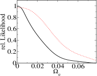
We propose a novel parameterization of the dark energy density. It is particularly well suited to describe a non-negligible contribution of dark energy at early times and contains only three parameters, which are all physically meaningful: the fractional dark energy density today, the equation of state today and the fractional dark energy density at early times. As we parameterize $\Omega_{\rm d}(a)$ directly instead of the equation of state, we can give analytic expressions for the Hubble parameter, the conformal horizon today and at last scattering, the sound horizon at last scattering, the acoustic scale as well as the luminosity distance. For an equation of state today $w_{0}<-1$, our model crosses the cosmological constant boundary. We perform numerical studies to constrain the parameters of our model by using Cosmic Microwave Background, Large Scale Structure and Supernovae Ia data. At $95\%$ confidence, we find that the fractional dark energy density at early times $\Omega_{\rm d}^{e}<0.06$. This bound tightens considerably to $\Omega_{\rm d}^{e}<0.04$ when the latest Boomerang data is included. We find that both the gold sample of Riess et. al. and the SNLS data of Astier et. al. when combined with CMB and LSS data mildly prefer $w_{0}<-1$, but are well compatible with a cosmological constant.

I Introduction

Current observations Astier:2005qq ; Riess:2004nr ; Spergel:2003cb ; Readhead:2004gy ; Dickinson:2004yr ; Tegmark:2003ud favor some form of dark energy that today comprises roughly 70% of the energy density of our Universe. One fundamental issue is whether dark energy is a true cosmological constant or time evolving Wetterich:fm ; Ratra:1987rm ; Caldwell:1997ii . In recent years, the notion of an evolving dark energy has been cast in various parameterizations Cooray:1999da ; Huterer:2000mj ; Corasaniti:2002vg ; Linder:2002et ; Chevallier:2000qy ; Upadhye:2004hh ; Wang:2004py of the equation of state $w(a)=p/\rho$ of dark energy. Yet such parameterizations are ill-suited to catch an intriguing possible feature of dark energy, namely that it could be present at an observable level even from as early as Big Bang Nucleosynthesis on. Such models would leave their imprints on the Cosmic Microwave Background Doran:2000jt , cosmic structure Doran:2001rw ; Bartelmann:2005fc and maybe even Big Bang Nucleosynthesis Wetterich:1994bg ; Bean:2001wt ; Muller:2004gu . There are some good points in favor of this scenario: if one links the presently small energy density of dark energy to the age of the Universe, one is led to attractor solutions Wetterich:fm ; Ratra:1987rm . Such scenarios occur in attempts to solve the cosmological constant problem from the point of view of dilatation symmetry Wetterich:fm and also in string theories.

Instead of parameterizing $w(a)$, we parameterize $\Omega_{\rm d}(a)$ directly. This will prove advantageous for two reasons: firstly, the amount of dark energy at early times is then a natural parameter and not inferred by integrating $w(a)$ over the entire evolution. Secondly, since the Hubble parameter is given by

$$\frac{H^{2}(a)}{H^{2}_{0}}=\frac{\Omega_{\rm m}^{0}a^{-3}+\Omega_{\rm rel.}^{0}a^{-4}}{1-\Omega_{\rm d}(a)},$$ (1)

a simple, analytic expression for $\Omega_{\rm d}(a)$ enables us to compute many astrophysical quantities analytically. In the above, $\Omega_{\rm rel.}^{0}$ is the fractional energy density of relativistic neutrinos and photons today, $\Omega_{\rm m}^{0}$ is the matter (dark and baryonic) fractional energy density and we assumed a flat Universe. For any parameterization of $\Omega_{\rm d}(a)$, the equation of state can of course be inferred from $\Omega_{\rm d}(a)$ via an analytic relation (see Equation (5)).

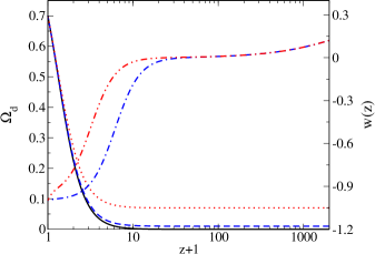
Figure 1: Evolution of the fractional dark energy density $\Omega_{\rm d}(z)$ and the equation of state $w(z)$ as a function of redshift. The solid (black) curve depicts the behavior for a $\Lambda$CDM cosmological constant model, in which $w_{0}=-1$ by definition and the amount of dark energy at early times tends to zero. In contrast, the dashed (blue) and dotted (red) curves are early dark energy models described by our parameterization (6). For the models depicted, we chose $w_{0}=-1$ and $\Omega_{\rm d}^{e}=0.01$ (blue, dashed), $\Omega_{\rm d}^{e}=0.07$ (red, dotted) respectively. In addition, we plot the equation of state $w$ for $\Omega_{\rm d}^{e}=0.01$ (blue, dashed-dotted) and $\Omega_{\rm d}^{e}=0.07$ (red, dashed-double-dotted)

II Parameterizing Dark Energy

As said, we would like to parameterize $\Omega_{\rm d}(a)$ to catch the important feature of early dark energy. In addition, the parameterization must involve only a restricted number of - physically meaningful - parameters (we will only require three: $\Omega_{\rm d}^{0}$, $w_{0}$ and $\Omega_{\rm d}^{e}$, see below). Equation (6) is our proposal which is derived from the following simple considerations: we start by observing that neglecting radiation, the fractional energy density of a cosmological constant evolves as

$$\Omega_{\Lambda}(a)=\frac{\Omega_{\rm d}^{0}}{\Omega_{\rm d}^{0}+\Omega_{\rm m}^{0}a^{-3}}.$$ (2)

Here, $a$ is the scale factor normalized to $a=1$ today, $\Omega_{\rm d}^{0}$ and $\Omega_{\rm m}^{0}$ are the fractional densities of dark energy and dark matter today and we assume a flat universe, i.e. $\Omega_{\rm m}^{0}+\Omega_{\rm d}^{0}=1$. The first generalization of this formula is to allow $w\neq-1$, which is achieved by Doran:2001rw

$$\Omega_{\rm d}(a)=\frac{\Omega_{\rm d}^{0}}{\Omega_{\rm d}^{0}+\Omega_{\rm m}^{0}a^{3w_{0}}}.$$ (3)

A straightforward attempt to include early dark energy is to simply add a term that is switched on at high redshifts and gives a basic contribution of the requested level

$$\Omega_{\rm d}(a)=\frac{\Omega_{\rm d}^{0}}{\Omega_{\rm d}^{0}+\Omega_{\rm m}^{0}a^{3w_{0}}}+\Omega_{\rm d}^{e}(1-a^{\alpha}).$$ (4)

where $\alpha>0$ is a parameter. It turns out, however, that this is insufficient, because the evolution of $\Omega_{\rm d}$ is connected to the equation of state $w$ by the relation Wetterich:2004pv

$$\left\{3w-\frac{a_{eq}}{a+a_{eq.}}\right\}\Omega_{\rm d}(1-\Omega_{\rm d})=-\textrm{d}\Omega_{\rm d}/\textrm{d}\ln a,$$ (5)

where $a_{eq}$ is the scale factor at matter-radiation equality. Demanding that $w(a=1)=w_{0}$, i.e. that the parameter $w_{0}$ should indeed have its usual meaning, one is led to conclude that an additional term is needed in the numerator and that $\alpha=-3w_{0}$. This yields the final form of our parameterization, namely

$$\Omega_{\rm d}(a)=\frac{\Omega_{\rm d}^{0}-\Omega_{\rm d}^{e}\left(1-a^{-3w_{0}}\right)}{\Omega_{\rm d}^{0}+\Omega_{\rm m}^{0}a^{3w_{0}}}+\Omega_{\rm d}^{e}\left(1-a^{-3w_{0}}\right).$$ (6)

In terms of the equation of state, going from today to the past, $w$ starts at $w_{0}$. It then crosses over to $w\approx 0$ during the matter dominated era. Defining the cross-over as $w=w_{0}/2$ and using Equations (5) and (6) and working to leading order in $\Omega_{\rm d}^{e}/\Omega_{\rm d}^{0}$, one obtains the cross-over scale factor

$$a_{c}\approx\left(\frac{\Omega_{\rm d}^{0}}{[1-\Omega_{\rm d}^{0}]\Omega_{\rm d}^{e}}\right)^{\frac{1}{3w_{0}}}.$$ (7)

We see from Equation (7), that increasing $\Omega_{\rm d}^{e}$ increases the cross-over scale factor, as expected. Likewise, a more negative $w_{0}$ also increases $a_{c}$, i.e. cross-over of $w$ occurs more recently. Finally, in the radiation dominated era, $w$ tends to $1/3$.

It is worth mentioning that our parameterization (6) is a monotonic function of $a$ for as long as

$$\Omega_{\rm d}^{e}\lesssim\frac{\Omega_{\rm d}^{0}}{2-\Omega_{\rm d}^{0}},$$ (8)

i.e. it stays monotonic even for rather large $\Omega_{\rm d}^{e}$. Hence, as $w=0$ during matter domination, we see that for $w_{0}<-1$, $w(a)$ will cross the cosmological constant boundary Feng:2004ad ; Vikman:2004dc ; Hu:2004kh ; Huey:2004jz ; Caldwell:2005ai . The evolution of $\Omega_{\rm d}$ and the corresponding $w$ are depicted in Figure 1.

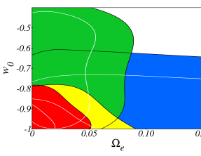
Figure 2: Constraints on the parameters $w_{0}$ and $\Omega_{\rm d}^{e}$ for different combinations of data sets. The blue region corresponds to the SNe Ia compilation of Riess et. al., the green region to WMAP + VSA + CBI + SDSS. The constraints obtained when combining all of these sets are shown in yellow. The result of adding the Boomerang data to this combined set is depicted in red. Black (white) lines enclose 95% (68%) confidence regions.

III Analytic results

A direct parameterization of $\Omega_{\rm d}(a)$ removes one integration otherwise necessary to compute the luminosity distance, sound horizon etc., because the Hubble parameter $H$ is given by Equation (1). Many cosmological quantities can then be computed analytically; the luminosity distance $d_{L}$, the horizon today and at last scattering $\tau_{0}$ and $\tau_{ls}$, the sound horizon $r_{s}$ and the acoustic scale $l_{A}$.

To derive an expression for the horizon today $\tau_{0}$, we neglect radiation in Equation (1), which leads to an error of less than $1\%$. Combining Friedmann’s Equation today and at arbitrary scale factor yields

$$\left(\frac{\textrm{d}a}{\textrm{d}\tau}\right)^{2}=H_{0}^{2}\left(\Omega_{\rm m}^{0}a+\Omega_{\rm d}(a)\right).$$ (9)

Inverting, drawing the root and separating the variables, one gets

$$\textrm{d}\tau=H_{0}^{-1}\int\textrm{d}a\,\sqrt{\frac{1-\Omega_{\rm d}(a)}{\Omega_{\rm m}^{0}\,a}}.$$ (10)

Using our parameterization Equation (6) and substituting $y=a^{-3w_{0}}$, one obtains

$$\tau_{0}=\frac{-1}{3w_{0}H_{0}\sqrt{\Omega_{\rm m}^{0}}}\int_{0}^{1}\frac{y^{-1-\frac{1}{6w_{0}}}\sqrt{1-\Omega_{\rm d}^{e}\left[1-y\right]^{2}}}{\sqrt{1+\frac{\Omega_{\rm d}^{0}}{\Omega_{\rm m}^{0}}y}}\textrm{d}y.$$ (11)

Expanding the root in the numerator yields

$$\tau_{0}=\frac{-1}{3w_{0}H_{0}\sqrt{\Omega_{\rm m}^{0}}}\int_{0}^{1}\frac{y^{-1-\frac{1}{6w_{0}}}\left(1-\frac{\Omega_{\rm d}^{e}}{2}\left[1-y\right]^{2}\right)}{\sqrt{1+\frac{\Omega_{\rm d}^{0}}{\Omega_{\rm m}^{0}}y}}\textrm{d}y.$$ (12)

We then split the integral in leading and next to leading order

$$\tau_{0}=\frac{-1}{3w_{0}H_{0}\sqrt{\Omega_{\rm m}^{0}}}\Biggl{\{}\int_{0}^{1}\frac{y^{-1-\frac{1}{6w_{0}}}}{\sqrt{1+\frac{\Omega_{\rm d}^{0}}{\Omega_{\rm m}^{0}}y}}\textrm{d}y\\ -\frac{\Omega_{\rm d}^{e}}{2}\int_{0}^{1}\frac{y^{-1-\frac{1}{6w_{0}}}[1-y]^{2}}{\sqrt{1+\frac{\Omega_{\rm d}^{0}}{\Omega_{\rm m}^{0}}y}}\textrm{d}y\Biggr{\}}.$$ (13)

Both integrals yield hypergeometric functions ${}_{2}F_{1}$ (up to $\Gamma$ functions). The final result may hence be expressed as

$$\tau_{0}=\frac{2}{H_{0}\sqrt{\Omega_{\rm m}^{0}}}\Biggl{\{}\,_{2}F_{1}\left(\frac{1}{2},\frac{-1}{6w_{0}},1-\frac{1}{6w_{0}},-\frac{\Omega_{\rm d}^{0}}{\Omega_{\rm m}^{0}}\right)\\ -\frac{\Omega_{\rm d}^{e}}{(2-\frac{1}{6w})(1-\frac{1}{6w})}\,_{2}F_{1}\left(\frac{1}{2},-\frac{1}{6w_{0}},3-\frac{1}{6w_{0}},-\frac{\Omega_{\rm d}^{0}}{\Omega_{\rm m}^{0}}\right)\Biggr{\}}.$$ (14)

In the limit that $\Omega_{\rm d}^{e}\to 0$, we recover the result for constant $w$ Doran:2001rw . The luminosity distance is computed in quite the same manner. Neglecting radiation, it is given by

$$d_{L}(z) = (1+z)\int_{0}^{z}\frac{\textrm{d}z^{\prime}}{H(z)}=(1+z)\int_{a(z)}^{1}\frac{a^{-2}\textrm{d}a}{H(a)}$$ (15)

$$= \int_{a(z)}^{1}\frac{a^{-1/2}\textrm{d}a}{H_{0}\sqrt{\Omega_{\rm m}^{0}}}\sqrt{\frac{1-\Omega_{\rm d}^{e}[1-a^{-3w_{0}}]^{2}}{1+\frac{\Omega_{\rm d}^{0}}{\Omega_{\rm m}^{0}}a^{-3w_{0}}}}.$$

The integral is in fact identical to the one in (11), but with $a(z)$ instead of $0$ as lower boundary. It seems feasible to derive an expression for $d_{L}(z)$ in terms of hypergeometric functions as well Gruppuso:2005xy . Yet such an expression would be rather lengthy. As the evaluation necessitates numerical methods in any case, we leave Equation (15) as it is.

At high redshift, $\Omega_{\rm d}^{e}$ simply scales the Hubble parameter by a constant factor. The Friedmann Equation (this time including radiation) then yields the horizon at last scattering Doran:2000jt

$$\tau_{ls}=\frac{2}{H_{0}}\left(\frac{1-\Omega_{\rm d}^{e}}{\Omega_{\rm m}^{0}}\right)^{1/2}\left[\sqrt{a_{ls}+\frac{\Omega_{\rm rel.}}{\Omega_{\rm m}^{0}}}-\sqrt{\frac{\Omega_{\rm rel.}}{\Omega_{\rm m}^{0}}}\right].$$ (16)

Here, $a_{ls}$ is the scale factor at recombination.

The sound horizon is given by

$$r_{s}(a)=\int_{0}^{a}\textrm{d}a\frac{\textrm{d}\tau}{\textrm{d}a}c_{s},$$ (17)

where the speed of sound is $c_{s}^{-2}=3(1+R^{-1})$. Here $R=\frac{4}{3}\frac{\rho_{\gamma}}{\rho_{b}}$ is the photon to baryon ratio. At redshifts where the speed of sound is appreciable and $r_{s}(a)$ receives contributions, $\Omega_{\rm d}(a)\approx\Omega_{\rm d}^{e}$ holds very well and we get again from the Friedmann Equation that

$$r_{s}=\frac{\sqrt{1-\Omega_{\rm d}^{e}}}{H_{0}}\int\frac{\textrm{d}a}{\sqrt{3\left(\Omega_{\rm m}^{0}a+\Omega_{\rm rel.}\right)\left(1+R^{-1}\right)}},$$ (18)

which can be integrated (similarly to Hu:1994uz ) to

$$r_{s}=\frac{4\sqrt{1-\Omega_{\rm d}^{e}}}{3H_{0}}\sqrt{\frac{\Omega_{\gamma}^{0}}{\Omega_{\rm b}^{0}\Omega_{\rm m}^{0}}}\\ \times\ln\frac{\sqrt{1+R^{-1}_{ls}}+\sqrt{R^{-1}_{ls}+R^{-1}_{equ.}}}{1+\sqrt{R^{-1}_{equ.}}}$$ (19)

Here, $R_{ls}$ and $R_{equ.}$ is the photon to baryon ratio as defined above at last scattering and matter-radiation equality respectively.

Finally, with $r_{s}$, $\tau_{0}$ and $\tau_{ls}$ given, the acoustic scale

$$l_{A}=\pi\frac{\tau_{0}-\tau_{ls}}{r_{s}},$$ (20)

can easily be computed.

IV Connection to Existing $w(a)$ Parameterizations

It may be worthwhile to relate our parameterization to the $w(a)$ parameterization of Corasaniti:2002vg

$$w^{Coras.}(a)=w_{0}+(w_{m}-w_{0})\times\frac{1+\exp(a_{c}/\Delta)}{1+\exp([a_{c}-a]/\Delta)}\\ \times\frac{1-\exp([1-a]/\Delta)}{1-\exp(1/\Delta)}.$$ (21)

This versatile parameterization is characterized by the equation of state of dark energy today $w_{0}$, the dark energy equation of state during earlier epochs $w_{m}$, a cross-over scale factor $a_{c}$ and a parameter $\Delta$ controlling the rapidity of this cross-over. In our case, $w_{0}$ has the same meaning, and $w_{m}=0$ always for our parameterization. We might roughly identify $a_{c}$ in (21) with (7). Using equations (5) and (6) and working to leading order in $\Omega_{\rm d}^{e}/\Omega_{\rm d}^{0}$, we also get an estimate of the width of the transition

$$\Delta_{c}\approx\left(1-3^{\frac{1}{3w_{0}}}\right)a_{c}.$$ (22)

We caution the reader that the accuracy of these expressions varies and hence the relation of our parameterization to that given in Equation (21) should be seen as a semi-quantitative statement.

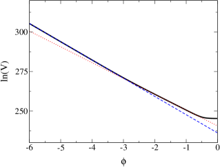
Figure 3: The logarithm of the potential, $\ln(V)$ as a function of $\varphi$ in units of $M_{\rm P}$ (solid line). The exponential potentials during radiation and matter domination are indicated by the dashed (blue) and dotted (red) line. The exponent in these cases is given by Equation (23). For this plot, we used $\Omega_{\rm d}^{e}=0.03$ and matter-radiation equality is at $\varphi_{equ.}=-2.66$. In the recent universe, the potential flattens, leading to $w\to-0.99$ which we picked for this plot.

V The Case of Scalar Dark Energy

If one uses our parameterization to describe the evolution of an (effective Doran:2002bc ) scalar dark energy field, then the constant $\Omega_{\rm d}\approx\Omega_{\rm d}^{e}$ at high redshifts implies an exponential potential for the scalar field. Indeed, the value of $\Omega_{\rm d}^{e}$ is that of an attractor solution for the potential Wetterich:fm

$$V(\varphi)=M_{\rm P}^{4}\exp\left(-\sqrt{3[1+w_{backg}]/{\Omega_{\rm d}^{e}}}\,\,\,\varphi\right),$$ (23)

where $M_{\rm P}$ is the reduced Planck mass and $w_{backg}$ is the equation of state of the components other than dark energy, i.e. $w_{backg}=1/3$ during radiation domination and $w_{backg}=0$ during matter domination. As $\Omega_{\rm d}^{e}=const.$ in our parameterization, we conclude that in terms of a scalar field potential, we have four “phases”. The potential (1) is an exponential potential during radiation domination, (2) moves over to a slightly less steep exponential potential during recombination, (3) stays with that exponential potential during matter domination and at late times (4) the potential flattens or – equivalently – the kinetic term Armendariz-Picon:2000dh ; Hebecker:2000zb changes. In Figure 3, we exemplify this behavior by plotting $\varphi$ in units of $M_{\rm P}$ vs. $\ln(V)$. For this plot, we have normalized $\varphi$ such that today $\varphi=0$.

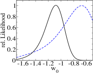
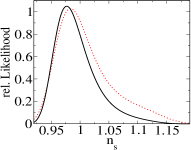
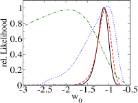
Figure 4: Upper left panel: Likelihood distribution for the equation of state $w_{0}$ today for a phantom model with $c_{s}^{2}=1$. The solid line is for WMAP + VSA + CBI + BOOMERANG + SDSS + SNe Ia, the dashed (blue) line is without Sne Ia data. At $1\sigma$ confidence, the full data gives $w_{0}=-1.08+0.14-0.17$. Upper right panel: Likelihood distribution for the scalar spectral index $n_{s}$ for a scalar field model. The solid line is for WMAP + VSA + CBI + BOOMERANG + SDSS + SNe Ia, the dotted (red) line is without Boomerang. At $1\sigma$ confidence, $n_{s}=0.98+0.04-0.03$. Lower left panel: Likelihood distribution for $\Omega_{\rm d}^{e}$ for a scalar field model. The solid line is for WMAP + VSA + CBI + BOOMERANG + SDSS+SNe Ia, the dotted (red) line is without Boomerang. At $2\sigma$ confidence, $\Omega_{\rm d}^{e}<0.04$ and $\Omega_{\rm d}^{e}<0.06$ respectively.  Lower right panel: Comparison of the likelihood distribution for the equation of state $w_{0}$ today for the gold set from Riess et. al. only (green, dot-dashed line) and the SNLS data only (blue, dotted line), and their combination with the CMB+LSS data: the dashed line (red) corresponds to CMB+LSS+Riess et. al., the solid (black) line to CMB+LSS+SNLS.

As said, our parameterization extends to phantom crossing models. For $w_{0}<-1$, there is a crossing from the phantom to the “canonical” dark energy regime. In this case, however, it seems impossible to describe the behavior using a single scalar field Vikman:2004dc ; Hu:2004kh ; Huey:2004jz ; Caldwell:2005ai ; Zhao:2005vj . For simulations of phantom crossing models, we chose to fix the rest frame speed of sound of dark energy to the speed of light $c_{s}^{2}=1$, which is compatible with the “microscopic” behavior of scalar dark energy models. Yet, from the point of view of fundamental physics, it seems ill-suited, because the entropy generation rate $\Gamma$ diverges. We nevertheless compute CMB and LSS constraints for phantom crossing models using $c_{s}^{2}=1$, because the detailed choice of $c_{s}^{2}$ seems to be of no significance for phenomenological studies using current data Caldwell:2005ai .

	$\Omega_{m}h^{2}$	$\Omega_{b}h^{2}$	$h$	$n_{s}$	$\tau$	$\ln(10^{10}A_{s})-2\tau$	$w_{0}$	$\Omega_{\rm d}^{e}$
BASE+SNE+B03	$0.143^{+0.007}_{-0.007}$	$0.023^{+0.001}_{-0.001}$	$0.69^{+0.02}_{-0.03}$	$0.98^{+0.04}_{-0.03}$	$0.13^{+0.08}_{-0.06}$	$2.90^{+0.03}_{-0.03}$	$\leq-0.82$	$\leq 0.04$
BASE+SNE	$0.143^{+0.008}_{-0.008}$	$0.024^{+0.002}_{-0.001}$	$0.68^{+0.03}_{-0.03}$	$0.98^{+0.05}_{-0.03}$	$0.15^{+0.10}_{-0.07}$	$2.89^{+0.04}_{-0.03}$	$\leq-0.82$	$\leq 0.06$
BASE+B03	$0.141^{+0.01}_{-0.01}$	$0.023^{+0.002}_{-0.001}$	$0.62^{+0.04}_{-0.05}$	$0.98^{+0.05}_{-0.03}$	$0.13^{+0.09}_{-0.07}$	$2.89^{+0.04}_{-0.03}$	$-0.65^{+0.18}_{-0.26}$	$\leq 0.04$
BASE	$0.142^{+0.01}_{-0.01}$	$0.024^{+0.002}_{-0.001}$	$0.61^{+0.04}_{-0.05}$	$0.98^{+0.06}_{-0.03}$	$0.14^{+0.10}_{-0.08}$	$2.88^{+0.04}_{-0.04}$	$-0.70^{+0.24}_{-0.28}$	$\leq 0.06$

Table 1: Parameter constraints for scalar dark energy models. BASE is WMAP+VSA+CBI+SDSS. All errors are $1\sigma$, upper bounds are $2\sigma$.

VI Simulation results

We added the parameterization (6) to Cmbeasy Doran:2003sy and computed constraints on cosmological parameters using a Markov Chain Monte Carlo approach Lewis:2002ah with the AnalyzeThis! package Doran:2003ua . The parameters we chose are the matter energy fraction $\Omega_{\rm m}^{0}h^{2}$, the baryon energy fraction $\Omega_{\rm b}^{0}h^{2}$, the hubble parameter $h$, optical depth $\tau$, scalar spectral index $n_{s}$, initial scalar amplitude $A_{s}$ using the observationally relevant combination $\ln(10^{10}A_{s})-2\tau$ as well as the dark energy parameters $w_{0}$ and $\Omega_{\rm d}^{e}$. We chose flat priors on all parameters and ran two kinds of models separately: scalar field dark energy models with $w_{0}>-1$ and phantom crossing models with $w_{0}\in[-5,0]$ and speed of sound $c_{s}^{2}=1$. We compare the predictions of the models with several combinations of data sets. The first set, CMB+LSS, consists of CMB data from WMAP Spergel:2003cb , VSA Dickinson:2004yr and CBI Readhead:2004gy , as well as LSS data from SDSS Tegmark:2003ud . For SNe Ia, we use the compilation by Riess et. al., Riess:2004nr . Motivated by recent comparisons of different SN Ia data sets Nesseris:2005ur ; Jassal:2006gf , we also take the first-year data from the SNLS Astier:2005qq into account when considering phantom crossing models.

	$\Omega_{m}h^{2}$	$\Omega_{b}h^{2}$	$h$	$n_{s}$	$\tau$	$\ln(10^{10}A_{s})-2\tau$	$w_{0}$	$\Omega_{\rm d}^{e}$
BASE+B03+SNLS	$0.15^{+0.01}_{-0.01}$	$0.023^{+0.001}_{-0.001}$	$0.70^{+0.02}_{-0.02}$	$0.96^{+0.03}_{-0.02}$	$0.10^{+0.07}_{-0.05}$	$2.94^{+0.04}_{-0.04}$	$-1.11^{+0.12}_{-0.14}$	$\leq 0.04$
BASE+SNLS	$0.15^{+0.01}_{-0.01}$	$0.023^{+0.001}_{-0.001}$	$0.70^{+0.03}_{-0.02}$	$0.96^{+0.03}_{-0.03}$	$0.11^{+0.08}_{-0.05}$	$2.95^{+0.04}_{-0.04}$	$-1.16^{+0.13}_{-0.17}$	$\leq 0.05$
BASE+SNE	$0.16^{+0.01}_{-0.01}$	$0.023^{+0.001}_{-0.001}$	$0.68^{+0.02}_{-0.02}$	$0.96^{+0.03}_{-0.02}$	$0.10^{+0.07}_{-0.05}$	$2.97^{+0.04}_{-0.05}$	$-1.16^{+0.19}_{-0.23}$	$\leq 0.06$
BASE+B03	$0.15^{+0.01}_{-0.01}$	$0.023^{+0.001}_{-0.001}$	$0.62^{+0.07}_{-0.06}$	$0.96^{+0.04}_{-0.02}$	$0.11^{+0.09}_{-0.06}$	$2.92^{+0.04}_{-0.04}$	$-0.68^{+0.24}_{-0.32}$	$\leq 0.04$
BASE+SNE+B03	$0.15^{+0.01}_{-0.01}$	$0.023^{+0.001}_{-0.001}$	$0.68^{+0.02}_{-0.02}$	$0.96^{+0.03}_{-0.02}$	$0.10^{+0.06}_{-0.05}$	$2.95^{+0.04}_{-0.04}$	$-1.08^{+0.13}_{-0.16}$	$\leq 0.04$

Table 2: Parameter constraints for phantom crossing models. BASE is WMAP+VSA+CBI+SDSS. All errors are $1\sigma$, upper bounds are $2\sigma$.

Turning first to the case of scalar field dark energy, our main results are shown in Figure 2 and Table 1. We see that the SNe Ia data and the CMB+LSS data give orthogonal information. While supernovae are insensitive to the amount of early dark energy $\Omega_{\rm d}^{e}$ but do constrain $w_{0}$, the opposite is true for the CMB+LSS set. Figure 2 also shows the likelihood contours obtained when adding the data from the 2003 flight of Boomerang Montroy:2005yx ; Piacentini:2005yq ; Jones:2005yb .

The stronger constraints on the amount of early dark energy from Boomerang are due to the particular suppression of power caused by $\Omega_{\rm d}^{e}$: the presence of dark energy suppresses the growth of linear fluctuations that are inside the horizon. The smaller the scale, the longer it suffered the suppression. This leads to a scale dependent red tilt of the spectra for all modes that enter after the scale of equality $k<k_{equ.}$. All modes $k>k_{equ.}$ were inside the horizon before equality and are suppressed by the same factor Caldwell:2003vp . An increase of $\Omega_{\rm d}^{e}$ is hence partially degenerate with a decrease of $n_{s}$. Now Boomerang alone prefers a rather red spectral index $n_{s}=0.86$ MacTavish:2005yk , whereas WMAP tends more towards $n_{s}\sim 1$ (see also the upper right panel of Figure 4). As far as early dark energy models with appreciable $\Omega_{\rm d}^{e}$ are concerned, WMAP forces them to have $n_{s}$ close to $1$, at least slightly larger than a comparable model with vanishing $\Omega_{\rm d}^{e}$. The relative lack of power of Boomerang at high multipoles does then disfavor those models with large $\Omega_{\rm d}^{e}$ and rather blue $n_{s}$.

Considering phantom crossing models, we use the CMB+LSS data, and the SNe Ia data from either Riess et. al. or the SNLS. In Table 2, we summarize the constraints. The comparison of the results for the equation of state parameter today, $w_{0}$, are shown in the upper left and lower right panels of Figure 4. We find that the SNLS data alone, in contrast to the set from Riess et. al., do not favor a value of $w_{0}<1$, which agrees with the findings in Nesseris:2005ur . This situation changes when combining the supernovae data with CMB+LSS, since the CMB essentially fixes $\Omega_{\rm m}^{0}h^{2}$. Without a free $\Omega_{m}^{0}$, both supernovae sets prefer a $w_{0}$ of slightly less than $-1$ Alam:2005pb ; Xia:2005ge ; Ichikawa:2005nb ; Cai:2005qm .

VII Conclusions

We introduced a new parameterization of dark energy. It is particularly well suited to describe models in which the dark energy density is non-negligible in the early Universe. Working with $\Omega_{\rm d}(a)$ instead of $w(a)$ facilitates the computation of quantities such as horizons, the luminosity distance and the acoustic scale. Using Markov Chain Monte Carlo simulations, we constrained the parameters of our model using the latest CMB, Sne Ia and LSS data. While the CMB is more sensitive to $\Omega_{\rm d}^{e}$, the opposite is true for Sne Ia, which are more sensitive to $w_{0}$. Adding the recent high multipole Boomerang data tightened the upper bound on $\Omega_{\rm d}^{e}$ considerably to $\Omega_{\rm d}^{e}<0.04$. However, our analysis only included linear fluctuations. As early dark energy models lead to more non-linear structure at higher redshifts compared to a cosmological constant Bartelmann:2005fc , it might well be that the upper bound turns into a detection in the future.

Acknowledgments We would like to thank Ben Gold for his helpful comments on the preprint.

VIII Appendix

The upper bound for $\Omega_{\rm d}^{e}$ with our parameterization in the scalar dark energy case is considerably higher than the one found in Doran:2005sn . This is a consequence of the longer period of time for which our parameterization mimics a cosmological constant, so that the influence of $\Omega_{\rm d}^{e}$ on the late-time evolution of the Universe induced by the choice of parameterization is minimized. It is then natural to ask if the bounds on $\Omega_{\rm d}^{e}$ in our model might relax if $\Omega_{\rm d}(a)$ behaved like a cosmological constant for higher redshifts. To answer this question, we generalize our parameterization Equation (6) by introducing an additional parameter $\gamma$ that controls the importance of the terms involving $\Omega_{\rm d}^{e}$ at late times,

$$\Omega_{\rm d}(a)=\frac{\Omega_{\rm d}^{0}-\Omega_{\rm d}^{e}\left(1-a^{-3w_{0}}\right)^{\gamma}}{\Omega_{\rm d}^{0}+\Omega_{\rm m}^{0}a^{3w_{0}}}+\Omega_{\rm d}^{e}\left(1-a^{-3w_{0}}\right)^{\gamma}.$$ (24)

When setting $\gamma=1$, this reduces to our parameterization (6), while increasing $\gamma$ shifts the departure from a cosmological constant-like behavior of $\Omega_{\rm d}(a)$ to higher redshifts. If we require $\Omega_{\rm d}(a)$ to stay monotonic, then $\gamma$ is bounded by

$$\gamma\lesssim\frac{\Omega_{\rm d}-\Omega_{\rm d}^{e}}{\Omega_{\rm d}^{e}(1-\Omega_{\rm d})}.$$ (25)

Repeating the Monte-Carlo analysis for the scalar dark energy case with this extended parameterization (24) at different values of $\gamma$ does not alter the constraints on the other parameters. It therefore suffices to use the simpler parameterization of Equation (6).

References

• (1) P. Astier et al., arXiv:astro-ph/0510447.
• (2) A. G. Riess et al. [Supernova Search Team Collaboration], Astrophys. J.  607, 665 (2004) [arXiv:astro-ph/0402512].
• (3) D. N. Spergel et al. [WMAP Collaboration], Astrophys. J. Suppl.  148, 175 (2003) [arXiv:astro-ph/0302209].
• (4) A. C. S. Readhead et al., Astrophys. J.  609 (2004) 498 [arXiv:astro-ph/0402359].
• (5) C. Dickinson et al., Mon. Not. Roy. Astron. Soc.  353 (2004) 732 [arXiv:astro-ph/0402498].
• (6) M. Tegmark et al. [SDSS Collaboration], Phys. Rev. D 69 (2004) 103501 [arXiv:astro-ph/0310723].
• (7) C. Wetterich, Nucl. Phys. B 302, 668 (1988)
• (8) B. Ratra and P. J. Peebles, Phys. Rev. D 37, 3406 (1988)
• (9) R. R. Caldwell, R. Dave and P. J. Steinhardt, Phys. Rev. Lett.  80, 1582 (1998)
• (10) A. R. Cooray and D. Huterer, Astrophys. J.  513, L95 (1999) [arXiv:astro-ph/9901097].
• (11) D. Huterer and M. S. Turner, Phys. Rev. D 64, 123527 (2001) [arXiv:astro-ph/0012510].
• (12) P. S. Corasaniti and E. J. Copeland, Phys. Rev. D 67, 063521 (2003) [arXiv:astro-ph/0205544].
• (13) E. V. Linder, Phys. Rev. Lett.  90, 091301 (2003).
• (14) M. Chevallier and D. Polarski, Int. J. Mod. Phys. D 10, 213 (2001) [arXiv:gr-qc/0009008].
• (15) A. Upadhye, M. Ishak and P. J. Steinhardt, arXiv:astro-ph/0411803.
• (16) Y. Wang and M. Tegmark, Phys. Rev. Lett.  92, 241302 (2004) [arXiv:astro-ph/0403292].
• (17) M. Doran, M. J. Lilley, J. Schwindt and C. Wetterich, Astrophys. J.  559, 501 (2001) [arXiv:astro-ph/0012139].
• (18) M. Doran, J. M. Schwindt and C. Wetterich, Phys. Rev. D 64, 123520 (2001) [arXiv:astro-ph/0107525].
• (19) M. Bartelmann, M. Doran and C. Wetterich, arXiv:astro-ph/0507257.
• (20) C. Wetterich, Astron. Astrophys.  301, 321 (1995) [arXiv:hep-th/9408025].
• (21) R. Bean, S. H. Hansen and A. Melchiorri, Phys. Rev. D 64, 103508 (2001) [arXiv:astro-ph/0104162].
• (22) C. M. Muller, G. Schafer and C. Wetterich, Phys. Rev. D 70, 083504 (2004) [arXiv:astro-ph/0405373].
• (23) C. Wetterich, Phys. Lett. B 594, 17 (2004) [arXiv:astro-ph/0403289].
• (24) B. Feng, X. L. Wang and X. M. Zhang, Phys. Lett. B 607, 35 (2005) [arXiv:astro-ph/0404224].
• (25) A. Vikman, Phys. Rev. D 71, 023515 (2005) [arXiv:astro-ph/0407107].
• (26) W. Hu, Phys. Rev. D 71 (2005) 047301 [arXiv:astro-ph/0410680].
• (27) G. Huey, arXiv:astro-ph/0411102.
• (28) R. R. Caldwell and M. Doran, Phys. Rev. D 72 (2005) 043527 [arXiv:astro-ph/0501104].
• (29) G. B. Zhao, J. Q. Xia, M. Li, B. Feng and X. Zhang, Phys. Rev. D 72, 123515 (2005) [arXiv:astro-ph/0507482].
• (30) A. Gruppuso and F. Finelli, arXiv:astro-ph/0512641.
• (31) W. Hu and N. Sugiyama, Astrophys. J.  444 (1995) 489 [arXiv:astro-ph/9407093].
• (32) M. Doran and J. Jaeckel, Phys. Rev. D 66, 043519 (2002) [arXiv:astro-ph/0203018].
• (33) C. Armendariz-Picon, V. Mukhanov and P. J. Steinhardt, Phys. Rev. Lett.  85, 4438 (2000) [arXiv:astro-ph/0004134].
• (34) A. Hebecker and C. Wetterich, Phys. Lett. B 497 (2001) 281 [arXiv:hep-ph/0008205].
• (35) M. Doran, JCAP 0510, 011 (2005) [arXiv:astro-ph/0302138].
• (36) A. Lewis and S. Bridle, Phys. Rev. D 66 (2002) 103511 [arXiv:astro-ph/0205436].
• (37) M. Doran and C. M. Mueller, JCAP 0409, 003 (2004) [arXiv:astro-ph/0311311].
• (38) S. Nesseris and L. Perivolaropoulos, arXiv:astro-ph/0511040.
• (39) H. K. Jassal, J. S. Bagla and T. Padmanabhan, arXiv:astro-ph/0601389.
• (40) T. E. Montroy et al., arXiv:astro-ph/0507514.
• (41) F. Piacentini et al., arXiv:astro-ph/0507507.
• (42) W. C. Jones et al., arXiv:astro-ph/0507494.
• (43) R. R. Caldwell, M. Doran, C. M. Mueller, G. Schaefer and C. Wetterich, Astrophys. J.  591 (2003) L75 [arXiv:astro-ph/0302505].
• (44) C. J. MacTavish et al., arXiv:astro-ph/0507503.
• (45) U. Alam and V. Sahni, arXiv:astro-ph/0511473.
• (46) J. Q. Xia, G. B. Zhao, B. Feng, H. Li and X. Zhang, arXiv:astro-ph/0511625.
• (47) K. Ichikawa and T. Takahashi, arXiv:astro-ph/0511821.
• (48) R. G. Cai, Y. Gong and B. Wang, arXiv:hep-th/0511301.
• (49) M. Doran, K. Karwan and C. Wetterich, JCAP 0511 (2005) 007 [arXiv:astro-ph/0508132].