A Modified Higher Order Godunov’s Scheme for Stiff Source Conservative Hydrodynamics

Abstract

We present an efficient second order accurate scheme to treat stiff source terms within the framework of higher order Godunov’s methods. We employ Duhamel’s formula to devise a modified predictor step which accounts for the effects of stiff source terms on the conservative fluxes and recovers the correct isothermal behavior in the limit of an infinite cooling/reaction rate. Source term effects on the conservative quantities are fully accounted for by means of a one-step, second order accurate semi-implicit corrector scheme based on the deferred correction method of Dutt et. al. We demonstrate the accurate, stable and convergent results of the proposed method through a set of benchmark problems for a variety of stiffness conditions and source types.

and

1 Introduction

We wish to solve the following system of partial differential equations describing a hydrodynamic flow with a stiff (energy) source term

$$\frac{\partial U}{\partial t}+\sum_{d=1}^{D}\frac{\partial F_{d}(U)}{\partial x_{d}}=S(U)$$ (1)

where $D$ is the dimensionality of the problem, $U,~{}F(U),~{}S(U)$ are the conservative variables, the conservative fluxes and the source term respectively, given by

$$U=\begin{pmatrix}\rho\\ \rho u_{1}\\ \vdots\\ \rho u_{D}\\ \rho E\end{pmatrix};\quad F_{d}(U)=\begin{pmatrix}\rho u_{d}\\ \rho u_{1}u_{d}+p\,\delta_{1d}\\ \vdots\\ \rho u_{D}u_{d}+p\,\delta_{Dd}\\ (\rho E+p)u_{d}\end{pmatrix};\quad S(U)=\begin{pmatrix}0\\ 0\\ \vdots\\ 0\\ \rho\Lambda(e,\rho)\end{pmatrix}.$$ (2)

In the above equations, $\rho$ is the density, $u_{d}$ the velocity in the $d$ direction, $E=e+\sum_{d=1}^{D}u_{d}^{2}/2$ is the total specific energy with, $e$, the specific internal energy. $\Lambda(e,\rho)$ is the term describing the source of specific internal energy.

In the following we consider the case of a stiff source term corresponding to an endothermic process, such as occurs in radiative losses. In addition, we restrict our analysis to source types that, at least near equilibrium, behave as a relaxation law. In the stiff case, the characteristic relaxation time scale for $S$ may be much smaller than the CFL time step for the hydrodynamic waves. For that reason, we would like to use a semi-implicit method, treating the stiff source term implicitly, while using an explicit method for the hyperbolic terms. However, the classical analysis of such fast endothermic processes shows that, in the limit as the relaxation time goes to zero, the gas can be described by the compressible flow equations with an isothermal equation of state [18]. Pember [14] showed that the use of formally second-order accurate semi-implicit methods such as Strang splitting, or a second-order Godunov predictor-corrector method could lead to a substantial loss of accuracy, due to inconsistencies between the the characteristic tracing step without sources and the effective limiting isothermal behavior. Such inconsistencies between the flux calculation with the limiting isothermal equation of state can lead to dramatic errors particularly at sonic points. Pember proposed various approaches to the problem based on classical relaxation theory. Roe and Hittinger [15] also addressed the issues raised here in relation to Godunov’s method with stiff relaxation. In their approach they split the equations based on a splitting of state space into stiff and non-stiff subspaces of the linearized source term to obtain in the stiff limit formulations similar to ours. However, neither Pember nor Roe and Hittinger did present a complete method that is second-order accurate in both the stiff and non-stiff limits, nor did they discuss the extension to more than one dimension.

The problem of hyperbolic system with stiff relaxation has also been considered by other authors in the past mostly for one-dimensional systems and within the framework of Runge-Kutta based methods of lines. In particular Jin [7] designed second order Runge-Kutta type splitting methods with the correct asymptotic limit. Jin and Levermore’s [8] developed a semidiscrete high resolution method which, in order to ensure the correct asymptotic behavior, employes a linear combination of the conservative fluxes for the homogeneous (i.e. without the relaxation term) and equilibrium system. The fluxes are computed with a higher order Godunov’s method and the scheme allows for a rapid transition between the stiff and nonstiff regimes. As the authors point out, however, the upwind property of the scheme is not strictly guaranteed for all stiffness conditions. Finally, Caflisch, Jin and Russo [2] developed a scheme for hyperbolic systems with relaxation that is uniformly accurate for various ranges of stiffness conditions (see also Ref. [9, 13]).

The aim of this paper is to build a higher order Godunov’s method that preserves the properties of robustness and accuracy across a variety of stiffness conditions thus avoiding the problems described in [14]. In particular, in order to preserve higher order accuracy, we aim for a semi-implicit method that corresponds to a standard second-order Godunov method of the appropriate hyperbolic problem for the stiff or non-stiff limits. To this end, we use second-order accurate deferred corrections method of a type presented in [5], to obtain a semi-implicit corrector that is a special case of the algorithms described in [12], although any implicit L-stable second-order one-step method would be acceptable. The main new idea in our work is contained in our treatment of the predictor step for computing the hyperbolic fluxes, based on the derivation of a local effective dynamics using Duhamel’s formula. This leads to an explicit predictor step that corresponds to that for a conventional second-order Godunov method for Eq. (1) in the limit where the relaxation time is comparable to or greater than the hydrodynamic CFL time step; and to a second-order Godunov method for the isothermal equations in the limit where the relaxation time is much smaller than the hydrodynamic time step. Our approach is similar to that used in [17] for obtaining a well-behaved numerical method for incompressible viscoelastic flows in both the viscous and elastic limits; however, the details there are quite different than those for the present setting.

The paper is organized as follows. In section 2 we describe a second order accurate, semi-implicit corrector method based on the deferred corrections ideas presented in [5, 12] to be used for the final source term update. In section 3, based on Duhamel’s formula, we work out a modified formulation of Godunov’s predictor step and flux calculation suitable for the case of stiff source terms. In section 4 we discuss stability issues for our approach, and Section 5 contains the extension of the method to the case in which the source term depends both on the gas density as well as the internal energy. In section 6 we test the performance of the code and demonstrate the accuracy of the method in various stiffness conditions. The paper concludes with section 7 where the main results of the paper are summarized.

2 Semi-Implicit Predictor-Corrector

Our time-discretization for the source terms is a single-step, second-order accurate scheme based on the deferred correction ideas in Dutt, Greengard & Rokhlin [5]. Given the system of equations (1)

$$\frac{\partial U}{\partial t}=-\nabla\cdot F+S(U)$$ (3)

we aim for a scheme in which an explicit approach is retained for the non-stiff conservative hydrodynamic term, $\nabla\cdot F$, and a implicit method is employed for the stiff part of the equation, $S$. The particular approach is a special case of a more general class of semi-implicit methods by Minion  [12]. Consider the first order system of ordinary differential equations (ODEs)

$$\frac{dY}{dt}=C(t,Y)$$ (4)

$$Y(t=0)=Y_{0}$$ (5)

with $Y\in\mathbb{R}^{n}$, $C:\mathbb{R}\times\mathbb{R}^{n}\rightarrow\mathbb{R}^{n}$. In [5], Eq. (4) is reformulated in terms of its equivalent Picard integral equation, to which a deferred corrections algorithm is iteratively applied. First an error is estimated according to

$$\tilde{\epsilon}(t)=Y_{0}+\int^{t}_{0}C\left[\tau,\tilde{Y}(\tau)\right]d\tau-\tilde{Y}(t)\hbox{ , }0\leq t\leq\Delta t$$ (6)

where, $\tilde{Y}(t)$, is an initial guess to the solution to be corrected iteratively. Then a correction is computed by solving the error equation for the correction $\delta(t)\equiv Y(t)-\tilde{Y}(t):$

$$\delta(t)=\int^{t}_{0}\left\{C\left[\tau,\tilde{Y}(\tau)+\delta(\tau)\right]-C\left[\tau,\tilde{Y}(\tau)\right]\right\}d\tau+\tilde{\epsilon}(t)$$ (7)

$${Y}(t)=\tilde{Y}(t)+\delta(t)\hbox{ , }0\leq t\leq\Delta t.$$

To complete the specification of the method, we need to choose a quadrature scheme to replace the integrals in time by sums over a finite number of points. The choice of quadrature method in the error calculation (6) and of the number of iterations determines the accuracy of the method. However, as noted in [5], the rate of convergence of the method is independent of the accuracy of the quadrature rule used in the correction calculation (7). In particular, for stiff systems, one uses a quadrature rule corresponding to backward Euler, replacing the integrand by its linear approximation. In the present case, we are only interested in second-order accuracy, so we can use the trapezoidal rule for the quadrature rule in the error calculation, and iterate only once.

Our semi-implicit method will correspond to solving a collection of ODEs, one at each grid point

$$\frac{dU}{dt}=S(U)-(\nabla\cdot\vec{F})^{n+\frac{1}{2}}$$ (8)

where we view the time-centered flux divergence as a constant source, whose computation using a modified Godunov method is decried below. Following [12], we solve the resulting collection of ODEs using the method described above. For our initial guess, we use

$$\tilde{U}=U_{0}+\left({\rm I}-\Delta t\nabla_{U}S|_{U_{0}}\right)^{-1}\left[S(U_{0})-(\nabla\cdot F)^{n+\frac{1}{2}}\right]\,\Delta t$$ (9)

where $U_{0}\equiv U(t_{0})$. In the above expression we have used backward Euler to estimate the effects of the source term and we have then Taylor expanded the implicit part of it into a linear form. This yields a second order accurate estimate in the sense that: $\tilde{U}-U(t_{0}+\Delta t)=O(\Delta t^{2})$. Based on Eq. (6) the error is then estimated as

$$\tilde{\epsilon}(\Delta t)=U_{0}+\frac{\Delta t}{2}\left[S(\tilde{U})+S(U_{0})\right]-\Delta t\,(\nabla\cdot F)^{n+\frac{1}{2}}-\tilde{U}$$ (10)

where we have used the trapezoidal rule to estimate the integral of the source term. The sought correction is obtained in implicit form by applying backward Euler to the integral in the correction equation (7)

$$\delta(\Delta t)=({\rm I}-\Delta t\nabla_{U}S|_{\tilde{U}})^{-1}\;\tilde{\epsilon}(\Delta t)$$ (11)

$$U(t_{0}+\Delta t)=\tilde{U}+\delta(\Delta t)$$ (12)

From Eq. (10)-(11) it is clear that the final solution will have a truncation error $O(\Delta t^{2})$ and global second order accuracy in time.

Clearly in the non-stiff limit, as the contribution from the term ‘$\Delta t\nabla_{U}S|_{U}$’ becomes negligible compared to those from ‘${\rm I}$’, the above scheme reduces to the usual second order accurate explicit formulation

$$U(t_{0}+\Delta t)=U_{0}-\Delta t\,(\nabla\cdot F)^{n+\frac{1}{2}}+\frac{\Delta t}{2}\left[S(\tilde{U})+S(U_{0})\right].$$ (13)

3 Effective Dynamics and a Modified Godunov’s Method

In order to compute the flux divergence $(\nabla\cdot\vec{F})^{n+\frac{1}{2}}$, we use the quasilinear form of the equations in primitive variables to extrapolate from cell centers to cell faces

$$\frac{\partial W}{\partial t}+\sum\limits_{d=1}^{D}A_{d}\frac{\partial W}{\partial x_{d}}=S^{(W)}(W)$$

$$S^{(W)}=\nabla_{U}W\,S(U).$$

In order to develop our formulation we will start using $W=(\rho,\boldsymbol{u},e)^{T}$, but will switch to the usual set of primitive variables later in Sec. 3.1.1. Hereafter, we will denote $S^{(W)}\equiv S$, dropping the superscript. We can also give the evolution along the Lagrangian trajectories

$$\frac{DW}{Dt}+\sum\limits_{d=1}^{D}A^{L}_{d}\frac{\partial W}{\partial x_{d}}=S(W)$$

$$A^{L}_{d}=A_{d}-u_{d}{\rm I}\hbox{ , }\frac{DW}{Dt}=\frac{\partial W}{\partial t}+(\boldsymbol{u}\cdot\nabla)W$$

We will derive from the quasilinear form of the equations a new system that includes, at least locally in time and state space, the effects of the stiff source terms on the hyperbolic structure, and use that quasilinear system to extrapolate from cell centers to faces in a Godunov method.

We first illustrate the approach for the case of a system of ODE. Consider the system of differential equations

$$\frac{dY}{dt}=BY+C(t),\quad Y(t_{0})=Y_{0}$$ (14)

$$Y:\mathbb{R}\rightarrow\mathbb{R}^{n},\quad B\in\mathbb{R}^{n\times n},\quad C:\mathbb{R}\rightarrow\mathbb{R}^{n}.$$ (15)

The evolution of the rate of change of $Y(t)$, namely $\delta Y\equiv Y(t)-Y_{0}$, is then described by $d\delta Y/dt=B\delta Y+BY_{0}+C(t)$ with $\delta Y(0)=0$. According to Duhamel’s formula,

$$\delta Y(t)=\int^{t}_{0}e^{(t-\tau)B}[BY_{0}+C(\tau)]\,d\tau.$$ (16)

When the properties of $B$ lead to a stiff numerical problem, the exponential term in the above integral is the one that changes most rapidly, motivating the approximation

$$\delta Y(t)\approx{\mathcal{I}}_{B}(\eta)\,[BY_{0}+C(0)]\,t$$ (17)

where

$${\mathcal{I}}_{B}(\eta)\equiv\eta^{-1}\,\int_{0}^{\eta}e^{\tau B}d\tau.$$ (18)

$$\frac{dY^{eff}}{dt}={\mathcal{I}}_{B}(\eta)\,[BY_{0}+C(0)].$$ (19)

In what follows, we will take $\eta=O(\Delta t)$. There are two distinguished limits to the effective equation. First, if $||B\eta||\ll 1$, then

$$\mathcal{I}_{B}(\eta)=I+O(\eta)$$ (20)

The second is when there is a single eigenmode of $B$ that is stiff relative to the time scale defined by $\eta$. Specifically, we assume that for some $v\in\mathbb{R}^{n}$

$$B=\tilde{B}-\lambda vv^{T}\quad\tilde{B}v=0,\thickspace v^{T}\tilde{B}=0$$ (21)

with

$$\lambda\eta\gg 1,\quad||\tilde{B}\eta||\ll 1.$$ (22)

Here $\lambda^{-1}$ is the fast time scale that is stiff relative to $\eta$. So we can write

$$\mathcal{I}_{B}(\eta)=(I-vv^{T})+O\left(\eta,\frac{1}{\lambda}\right)$$ (23)

and

$$\mathcal{I}_{B}(\eta)B=\tilde{B}+O\left(\eta,\frac{1}{\lambda}\right).$$ (24)

In this case, $\mathcal{I}_{B}(\eta)$ projects out the stiff dynamics, leaving only processes that are resolved on the $O(\eta)$ timescale.

We can use the effective equation (19) with $\eta=\Delta t$ to compute a first-order accurate predictor step in a second-order accurate predictor-corrector.

$$Y^{\rm eff}(\Delta t)=Y(0)+\mathcal{I}(\Delta t)(BY(0)+C(0))\Delta t$$ (25)

Then

$$\begin{split}Y^{\rm eff}(\Delta t)-Y(\Delta t)&=O(\Delta t^{2})~{}~{}~{}~{}~{}~{}~{}~{}~{}~{}\text{ if (\ref{ib1:eq}) holds}\\ &=\left(\Delta t^{2}+\frac{\Delta t}{\lambda}\right)~{}~{}~{}\text{ if (\ref{ib2:eq}) holds}\end{split}$$ (26)

We apply this idea to the dynamics along Lagrangian trajectories. We define

$$\delta W=W[\boldsymbol{x}(t),t]-W[\boldsymbol{x}(t_{0}),t_{0}]\equiv W-W_{0}$$ (27)

and

$$\frac{D\delta W}{Dt}+G=S_{0}+\dot{S}_{0}\delta W$$ (28)

$$G=\sum\limits^{D}_{d=1}A^{L}_{d}\frac{\partial W}{\partial x_{d}}$$ (29)

We have linearized the source term around the value of the state at the beginning of the Lagrangian trajectory, with $\dot{S}=\nabla_{W}\cdot S$. By applying Duhamel’s formula to Eq. (28) we obtain

$$\delta W(t)=\int_{t_{0}}^{t}e^{(t-\tau)\dot{S}_{0}}(-G+S_{0})d\tau.$$ (30)

Following similar reasoning to the ODE case, we obtain

$$\frac{DW^{\rm eff}}{Dt}+\left(\sum_{d=1}^{D}{\mathcal{I}}_{\dot{S}_{0}}(\eta)\,A_{d}^{L}\,\frac{\partial W}{\partial x_{d}}\right)={\mathcal{I}}_{\dot{S}_{0}}(\eta)\,S_{0}.$$ (31)

3.1 Characteristic Analysis

We will use the quasilinear system (31) with $(\eta)=\Delta t/2$ to compute the Godunov predictor step. In the non-stiff limit, this leads to an $O(\Delta t^{2})$ error in the predicted values at cell faces which is sufficient for second-order accuracy in the overall method. In order to do that, we need to analyze the hyperbolic structure of those equations. Without loss of generality in the following subsections we still consider the 1-dimensional case. Also, in this section we will focus on the case $\Lambda_{\rho}\equiv\partial\Lambda/\partial\rho=0,\Lambda_{e}\equiv\partial\Lambda/\partial e\neq 0$; we will discuss the more general case in Sec. 5. With this choice of $\dot{S}_{0}$, from Eq. (18) we obtain

$${\mathcal{I}}_{\dot{S}_{0}}(\Delta t/2)=\begin{pmatrix}1&0&0\\ 0&1&0\\ 0&0&\alpha\end{pmatrix}$$ (32)

where

$$\alpha=\frac{e^{\frac{1}{2}\Lambda_{e}\Delta t}-1}{\frac{1}{2}\Lambda_{e}\Delta t}~{}~{}~{}~{}~{}~{}~{}~{}~{}~{}0<\alpha<1.$$ (33)

Thus, the presence of a stiff source term leads us to the transformations:

$$A\equiv A^{L}+u{\rm I}\rightarrow A^{\rm eff}=\begin{pmatrix}0&\rho&0\\ \frac{1}{\rho}\left(\frac{\partial p}{\partial\rho}\right)_{e}&0&\frac{1}{\rho}\left(\frac{\partial p}{\partial e}\right)_{\rho}\\ 0&\alpha\frac{p}{\rho}&0\end{pmatrix}+u{\rm I}.$$ (34)

3.1.1 Modified eigenvalues

Characteristic analysis of the matrix $A^{\rm eff}$ leads to the characteristic equation

$$\det(A^{\rm eff}-\lambda{\rm I})=(\lambda-u)\left[(\lambda-u)^{2}-\alpha\frac{p}{\rho^{2}}\left(\frac{\partial p}{\partial e}\right)_{\rho}-\left(\frac{\partial p}{\partial\rho}\right)_{e}\right]=0$$ (35)

which admits the the familiar solutions

$$\lambda_{0}=u,\quad\lambda_{\pm}=u\pm\left[\alpha\frac{p}{\rho^{2}}\left(\frac{\partial p}{\partial e}\right)_{\rho}+\left(\frac{\partial p}{\partial\rho}\right)_{e}\right]^{\frac{1}{2}}.$$ (36)

It appears from the above equation that the presence of the source term alters the sound speed according to

$$c_{s}=\left(\frac{\partial p}{\partial\rho}\right)_{s}^{\frac{1}{2}}\rightarrow c_{\rm eff}=\left[\alpha\frac{p}{\rho^{2}}\left(\frac{\partial p}{\partial e}\right)_{\rho}+\left(\frac{\partial p}{\partial\rho}\right)_{e}\right]^{\frac{1}{2}}.$$ (37)

For a $\gamma$-law equation of state, we have

$$p=(\gamma-1)\rho e$$ (38)

$$c_{\rm eff}=\left\{\left[\alpha\left(\gamma-1\right)+1\right]\,\frac{p}{\rho}\right\}^{\frac{1}{2}}.$$ (39)

Thus, in the limit of a negligible source term, $\alpha\rightarrow 1$, $c_{\rm eff}\rightarrow(\gamma p/\rho)^{1/2}$ and the polytropic behavior is recovered. However, in the limit of a stiff source term, $\alpha\rightarrow 0$, $c_{\rm eff}\rightarrow(p/\rho)^{1/2}$ and the isothermal regime is approached. This is also apparent from the expression for the rate of change of the internal energy along Lagrangian trajectories

$$\frac{De}{Dt}=-\alpha\frac{p}{\rho}\frac{\partial u}{\partial x},$$ (40)

suggesting the limit, $de\rightarrow 0$ as $\alpha\rightarrow 0$. Notice that in our approach we retain the polytropic form of the equation of state $p=(\gamma-1)\rho e$, $\gamma\neq 1$, but we avoid differentiating it when the presence of source terms must be taken into account. Based on Eq. (40) the pressure change is found to be

$$\frac{Dp}{Dt}=c^{2}_{\rm eff}\,\frac{D\rho}{Dt}=-\rho\,c^{2}_{\rm eff}\,\frac{\partial u}{\partial x}.$$ (41)

Finally, we note that in general, in $D-$dimensions, the above analysis applies unaltered to the linear operator, $A^{\rm eff}_{d}$, for each direction, $d$, after properly transforming $u\rightarrow u_{d},~{}x\rightarrow x_{d}$. In addition, $D-1$ equations are added describing the passive transport of momentum components perpendicular to the $d$ direction, and the eigenvalue $\lambda_{0}$ acquires multiplicity $D$.

3.1.2 Modified Eigenvectors

Given Eq. (41) we can now replace internal energy with pressure and find out the expression for the eigenvectors for the usual set of primitive variables. This reads

$$W=(\rho,u,p,s)^{\bf T},$$ (42)

where in addition to density, velocity and pressure, we have also included the specific entropy, $s=p\rho^{-\gamma}$ (useful, e.g., for the case of hypersonic flows [11]). The change in specific entropy is given by

$$\frac{Ds}{Dt}=\rho^{-\gamma}\,\left(\frac{Dp}{Dt}-c^{2}\,\frac{D\rho}{Dt}\right)=-\rho^{1-\gamma}\,\left(c^{2}_{\rm eff}-c^{2}\right)\,\frac{\partial u}{\partial x}\equiv-\rho^{1-\gamma}\,\delta_{c^{2}}\,\frac{\partial u}{\partial x}$$ (43)

The linear operator is

$$A^{\rm eff}=\begin{pmatrix}0&\rho&0&0\\ 0&0&\rho^{-1}&0\\ 0&\rho c^{2}_{\rm eff}&0&0\\ 0&\delta_{c^{2}}\rho^{1-\gamma}&0&0\end{pmatrix}+u{\rm I}.$$ (44)

The extra variable ‘$s$’ results in an additional eigenvalue, $\lambda=u$, for the operator $A^{\rm eff}$. The set of left and right eigenvectors are given respectively by

$$l_{1}=\left(0,-\frac{\rho}{2c_{\rm eff}},\frac{1}{2c^{2}_{\rm eff}},0\right)$$ (45)

$$l_{2}=\left(1,0,-\frac{1}{c^{2}_{\rm eff}},0\right)$$ (46)

$$l_{3}=\left(0,0,-\frac{\delta_{c^{2}}}{\rho^{\gamma}c^{2}_{\rm eff}},1\right)$$ (47)

$$l_{4}=\left(0,\frac{\rho}{2c_{\rm eff}},\frac{1}{2c^{2}_{\rm eff}},0\right)$$ (48)

$$r_{1}=\begin{pmatrix}1\\ -\frac{c_{\rm eff}}{\rho}\\ c^{2}_{\rm eff}\\ \delta_{c^{2}}\rho^{-\gamma}\end{pmatrix};\quad r_{2}=\begin{pmatrix}1\\ 0\\ 0\\ 0\end{pmatrix};\quad r_{3}=\begin{pmatrix}0\\ 0\\ 0\\ 1\end{pmatrix};\quad r_{4}=\begin{pmatrix}1\\ \frac{c_{\rm eff}}{\rho}\\ c^{2}_{\rm eff}\\ \delta_{c^{2}}\rho^{-\gamma}\end{pmatrix}.$$ (49)

3.2 Godunov Predictor in One Dimension

With the operator $A^{\rm eff}$ and the sets of left and right eigenvectors that we have worked out in the previous section, the Godunov predictor step is carried out as usual as follows.

First the local slopes are defined. In particular at each point left and right one-sided slopes as well as cell centered slopes are evaluated and then a final choice on the local slope $\Delta W_{i}$ is defined by using van Leer limiter. The upwind, time averaged left $(-)$ and right $(+)$ states at cell interfaces due to fluxes in the normal direction, $d$, are then reconstructed as:

$$W_{i,\pm}=W^{n}_{i}+\frac{1}{2}\left(I-\frac{\Delta t}{\Delta x}A^{\rm eff}_{i}\right)P_{\pm}(\Delta W_{i})$$ (50)

where

$$P_{\pm}(W)=\sum_{\pm\lambda_{k}>0}(l_{k}\cdot W)\cdot r_{k}.$$ (51)

The source term component is likewise accounted for as

$$W_{i,\pm,d}=W_{i,\pm,d}+\frac{\Delta t}{2}{\mathcal{I}}_{\dot{S}_{0}}(\Delta t/2)S_{0}.$$ (52)

The fluxes at the cell faces $F_{i+\frac{1}{2}}$ are computed by solving the Riemann problem with left and right states given by $\left(W_{i,+},W_{i+1,-}\right)$ to obtain $W^{n+\frac{1}{2}}_{i+\frac{1}{2}}$ and computing $F_{i+\frac{1}{2}}=F\left(W^{n+\frac{1}{2}}_{i+\frac{1}{2}}\right)$.

To modify this procedure to account for the effective dynamics, we use the characteristic analysis of the effective dynamics to perform each of the three steps. The projection operator and any limiting in characteristic variables is done using the eigenvectors and eigenvalues for the effective dynamics derived in Sec. 3.1. Typical approximate Riemann solvers use weak-wave approximations to compute the jumps, which only require the linearized jump relations provided by the characteristic analysis for the effective dynamics. For the case of a polytropic gas, one can use more nonlinear approximate Riemann solvers, e.g. two shock approximations, to compute the jump relations, treating $1+\alpha(\gamma-1)$ as an effective polytropic $\gamma$. This is done for the results presented here. Finally, any entropy fixes required to eliminate rarefaction shocks require only the sound speed, for which we again use $c_{\rm eff}$.

3.3 Extension to More than One Dimension

For directionally unsplit schemes in $D$ dimensions an additional step is required in order to correct the time-averaged left/right states at cell interfaces, $W_{i,\pm,d}$ in Eq. (52), for the effects of $D-1$ fluxes perpendicular to the cell interface normal direction. Based on Eq. (31) the effect of the stiff source term would be accounted for by carrying out for each additional direction, $d$, a transformation

$$A_{d}\rightarrow{\mathcal{I}}_{\dot{S}_{0}}(\Delta t/2)A_{L,d}+u_{d}{\rm I}\equiv A^{\rm eff}_{d}$$ (53)

analogous to that described in Eq. (34). In the method proposed by [4, 16] the corrections due to transverse fluxes are computed according to a conservative scheme. For example in two dimensions

$$W_{{i,j},\pm,x}=W_{{i,j},\pm,x}-\frac{\Delta t}{2\Delta y}\nabla_{U}W\;\left(F^{y}_{{i,j+\frac{1}{2}}}-F^{y}_{{i,j-\frac{1}{2}}}\right)$$ (54)

where the input $W_{{i,j},\pm,x}$ is computed using a one-dimensional Godunov calculation as in the previous section, as are the fluxes $F^{y}_{{i,j+\frac{1}{2}}}$. The notation in Eq. (54) indicates that primitive variables are converted into conservative variables which are then updated through conservative fluxes and then converted back into primitive form. Thus, if we indicate with $\Delta F^{y}_{\rho E}$ the undivided flux difference in the $d$ direction for the total energy, the above transformations imply the following correction

$$\Delta F^{y}_{\rho E}\rightarrow\Delta F^{y}_{\rho E}+(\alpha-1)\,\frac{1}{2}\left(p_{i,j+\frac{1}{2}}+p_{i,j-\frac{1}{2}}\right)\,\left(u_{y,i,j+\frac{1}{2}}-u_{y,i,j-\frac{1}{2}}\right)$$

This modification leads to a pressure change in accord to Eq. (41). Similarly, the entropy flux difference is modified as

$$\Delta F^{y}_{\rho s}\rightarrow\Delta F^{y}_{\rho s}+(\alpha-1)\,(\gamma-1)\,\frac{1}{2}\left[\left(\rho s\right)_{i,j+\frac{1}{2}}+\left(\rho s\right)_{i,j-\frac{1}{2}}\right]\,\left(u_{y,i,j+\frac{1}{2}}-u_{y,i,j-\frac{1}{2}}\right).$$

4 Stability Considerations

The method outlined above satisfy a number of conditions required for numerical stability. It is easy to see from Eq. (40) that, as $d\Lambda/de\rightarrow-\infty$, the internal energy decays rapidly to its equilibrium value, and thereafter remains constant, at that value. Inspection of the characteristic analysis shows that, in this limit, no information is carried along the entropy wave corresponding to the eigenvalue $\lambda_{0}$. This means that the system of equations (1) effectively reduces to the equilibrium system in which the internal energy is fixed at its equilibrium value. In addition, Eq. ( 36) and (37) indicate that the so called subcharacteristic condition for the characteristic speeds at equilibrium is always satisfied. That is

$$\lambda_{-}<\lambda^{\rm eff}_{-}<\lambda_{0}<\lambda^{\rm eff}_{+}<\lambda_{+}$$ (55)

where $\lambda^{\rm eff}_{+,-}$ and $\lambda_{+,0,-}$ are the equilibrium and frozen eigenvalues, respectively. The above condition, while being necessary for the stability of our linearized system [19], also guarantees that the numerical solution tends to the solution of the equilibrium equation as the relaxation time tends to zero [3]. Since the structure of the equations and the numerical framework, including the Riemann solver, remain basically unaltered with respect to classic Godunov’s schemes except for the modification of the sound speed, one expects the usual stability analysis to apply. The latter implies the familiar CFL condition on the time step

$$\max(|\lambda_{*}|)\frac{\Delta t}{\Delta x}\leq 1\hskip 28.45274pt*=-,0,+.$$ (56)

As for the step involving the source update, stability analysis for deferred correction methods of the type adopted here was carried out through numerical experiments by Dutt et al. [5]. Minion [12] extends such considerations to the case of semi-implicit schemes as the one adopted here. While the stability and convergence properties of such schemes have not been fully elucidated analytically, the analysis of these authors suggest that they are in general very satisfactory and competitive with commonly employed modern integration schemes.

Here we show that, provided that the CFL condition in Eq. (56) is satisfied, our method is A-stable, in the sense further specified below. To demonstrate this we apply the method to the following model problem [2]

$$\frac{dY(t)}{dt}=AY+BY$$

$$Y(0)=1$$

where $Y:\mathbb{R}\rightarrow\mathbb{C}$ and $A,B\in\mathbb{C}$ and represent the non-stiff and stiff part of the equation, respectively. Using the notation

$$Y^{n+1}=P(z_{1},z_{2})\,Y^{n},$$

where $P(z_{1},z_{2})$ is the operator corresponding to the proposed method, $z_{1}=A\Delta t$, $z_{2}=B\Delta t$, the stability region of the method, $P$, is defined as the region $S_{P}=\{z_{1},z_{2}\in\mathbb{C}:\lvert P(z_{1},z_{2})\rvert<1\}$. A method, $P$, is A-stable if $S_{P}$ includes the plane $\mathbb{C}_{-}\equiv\{z\in\mathbb{C}:\mathbb{R}(z)<0\}$. Inspection of equations (9)-(12) and simple algebraic manipulation lead to the expression

$$P(z_{1},z_{2})=[1+P_{h}(z_{1})]\,\frac{1-\dfrac{3}{2}z_{2}}{(1-z_{2})^{2}}+\frac{\dfrac{z_{2}}{2}}{1-z_{2}}$$ (57)

where $P_{h}$ is the hydrodynamic operator given by Godunov’s method. Using the CFL conditions, which ensures $\lvert P(z_{1},0)\rvert=\lvert 1+P_{h}(z_{1})\rvert<1$, we find:

$$\lvert P(z_{1},z_{2})\rvert^{2}<\frac{\left\lvert 1-z_{2}-\dfrac{z_{2}^{2}}{2}\right\rvert}{(1-z_{2})^{4}}<1~{}~{}\forall z_{2}:\mathbb{R}(z_{2})<0.$$ (58)

5 Extension to the Case $\Lambda_{\rho}\neq 0$

When the source term depends on both the internal energy and the gas density, $\Lambda_{\rho}\neq 0$ and we obtain

$${\mathcal{I}}_{\dot{S}_{0}}(\Delta t)=\begin{pmatrix}1&0&0\\ 0&1&0\\ (\alpha-1)\,\frac{\Lambda_{\rho}}{\Lambda_{e}}&0&\alpha\end{pmatrix}$$ (59)

with $\alpha$ defined in Eq. (33). As a result

$$A^{\rm eff}=\begin{pmatrix}0&\rho&0\\ \frac{1}{\rho}\left(\frac{\partial p}{\partial\rho}\right)_{e}&0&\frac{1}{\rho}\left(\frac{\partial p}{\partial e}\right)_{\rho}\\ 0&(\alpha-1)\frac{\Lambda_{\rho}}{\Lambda_{e}}\rho+\alpha\frac{p}{\rho}&0\end{pmatrix}+u{\rm I}$$ (60)

and the sound speed is now given by

$$c_{\rm eff}=\left\{\left[(\alpha-1)\frac{\Lambda_{\rho}}{\Lambda_{e}}\rho+\alpha\frac{p}{\rho}\right]\frac{1}{\rho}\,\left(\frac{\partial p}{\partial e}\right)_{\rho}+\left(\frac{\partial p}{\partial\rho}\right)_{e}\right\}^{\frac{1}{2}}.$$ (61)

Since $\alpha<1$ the term in squared brackets can become negative and the sound speed imaginary. This behavior is related to the fact that when $\Lambda_{\rho}\neq 0$ the gas is prone to thermal instability so that the scheme cannot be simply generalized without taking into account the specific properties of the source term. In general one cannot expect an implicit method to work properly except in the case of a system with a stable solution. For a $\gamma-$law equation of state, Eq. (38), $c_{\rm eff}^{2}>0$ requires

$$\frac{e}{\rho}\,\frac{\Lambda_{e}}{\Lambda_{\rho}}>\frac{1-\alpha}{\alpha\,(\gamma-1)}$$ (62)

which is reminiscent of the thermal stability criterion [6], in which case the term on the right-hand-side is 1. In both the stiff limit and non-stiff limits the RHS in Eq. (62) is of order $-\Lambda_{e}\,\Delta t\gg 1$, indicating the potential for triggering thermal instability of ‘numerical nature’. For example, consider a source of the form $\Lambda(\rho,e)=\rho^{n}\,\tilde{\Lambda}(\rho,e)$, so that

$$\Lambda_{\rho}(\rho,e)=n\rho^{-1}\,\Lambda(\rho,e)+\rho^{n}\,\tilde{\Lambda}_{\rho}(\rho,e).$$ (63)

In general the former term can take both positive and negative values. So even though it vanishes at equilibrium, its effect is destabilizing and should be resolved in time. Depending on the definition of $\Lambda$, it is possible that $\tilde{\Lambda}_{\rho}\geq 0$. Only in this case is the latter term stabilizing and should contribute to the sound speed in Eq. (61).

So our approach is to decouple any destabilizing component of $\Lambda_{\rho}$, which we indicate with $\Lambda_{\rho,<}$, from the characteristic analysis and associate it explicitly with the source term so that its effect does not enter the sound speed. In this case one would have to add a term

$$\Delta p=\rho\Delta e=-(\alpha-1)\,\frac{\Lambda_{\rho,<}}{\Lambda_{e}}\,\rho^{2}\,\left(\nabla\cdot{\bf u}\right)\,\frac{\Delta t}{2}$$ (64)

to the pressure component of the right hand side of Eq. (52). In order to preserve second order accuracy, one would require that the above term is resolved in time, i.e. the time step is sufficiently small that $\Delta e<e$. The restriction placed by Eq. (52) depends on the shape of the source function. However, near equilibrium it does not play any role because by definition to zeroth order the source term is zero. In fact we find that in all test cases with a density dependent source explored below, including the one in section 6.3, the condition (52) never constrained the time step.

6 Tests

In this section we test the performance of the proposed method in terms of both accuracy and robustness. As for the accuracy we consider a set of one dimensional problems for which the analytic solution is known. In particular, we use the test problems in [14] for an isothermal rarefaction fan and an isothermal shock wave and consider a flow with a stiff relaxation term in the limit in which the relaxation time approaches zero. We then consider the case of a sinusoidal perturbation with wave-vector both parallel (1-D) and skew (2-D) with respect to the x-axis, and prove the second order accuracy of the scheme for a variety of stiffness conditions. This we show both for the case in which the source term does or does not depend on density. As for the robustness of the method, we turn to multidimensional problems involving strong shocks and large spatial gradients. In particular we consider the interaction of a strong shock with a spherical cloud, again assuming a variety of stiffness conditions. The aim of the tests is to prove the code performance in the case of complex and computationally more challenging calculations.

As for the source term, in the following we mostly present results based on a relaxation law of the form

$$\Lambda=-{\rm K}\,\rho^{\zeta}\,\left[e-e_{0}\,\left(\frac{\rho}{\rho_{0}}\right)^{\eta}\right]$$ (65)

where $K$ is the heat transfer coefficient and the internal energy, $e$, is related to pressure and density by the equation of state (38), and $\zeta$ and $\eta$ are parameters. When $\zeta=\eta=0$ the relaxation law expressed by Eq. (65) reduces to the case studied in [14] and in the limit $K\rightarrow\infty$ it enforces isothermality.

We test the case of a density dependent source term, by setting either $\zeta$ or $\eta$, or both parameters, to a non zero value. Only the latter case is reported here although in all cases we obtain consistent results in terms of convergence and accuracy. When $\eta\neq 0$, Eq. (65) forces the system towards an equilibrium configuration described by polytropic-like equation of state in which $e=e_{0}\,(\rho/\rho_{0})^{\eta}$. Thus, when $\eta>0$, Eq. (61) implies an effective adiabatic index that, as it should be, tends to $(1+\eta)$, as $\alpha\rightarrow 0$.

6.1 Riemann Problems

We first consider one-dimensional Riemann problems described by the following initial conditions

$$(\rho,u,p)[x,t=0]=\left\{\begin{array}[]{lll}(\rho_{l},u_{l},p_{l})&\mbox{if}&x\leq 0.5\\ (\rho_{r},u_{r},p_{r})&\mbox{if}&x>0.5\end{array}\right.$$ (66)

and with a source term described by Eq. (65). Following [14] we adopt

$$K=10^{8}$$ (67)

$$e_{0}=\frac{p_{l,r}}{\rho_{l,r}\,(\gamma-1)}=1$$ (68)

$$\gamma=1.4$$ (69)

$$\Delta x=2.5\times 10^{-3}.$$ (70)

The stiff nature of the problem is apparent as K${}^{-1}\ll\Delta x/c_{\rm eff}$, i.e. the relaxation time is much shorter than the hydrodynamic time scale.

6.1.1 Isothermal Rarefaction

Figure 1: Isothermal rarefaction wave. From top to bottom: density, velocity and pressure solutions, respectively. Open dots and solid line indicate the numerical and analytic solution, respectively. The initial conditions are given in Eq. (71) with $u_{l}=-0.8$. A mesh size $\Delta x=2.5\times 10^{-3}$ was employed.

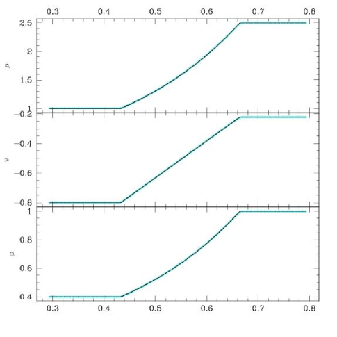
We begin by setting the state variables to the values

$$\begin{array}[]{lll}\rho_{l}=1.0,&p_{l}=0.4,&u_{l}=-0.8\\ \rho_{r}=2.5,&p_{r}=1.0,&u_{r}=u_{l}+0.5795\end{array}$$ (71)

representing an isothermal rarefaction in the $\lambda_{+}$ characteristic family. For the calculation we employ a grid with $N_{cell}=400$ grid cells [14]. The results from the code (open dots) are illustrated together with the analytic solution (solid line) in Fig. 1. From top to bottom the plot shows the density, velocity and pressure solutions at time $t=0.4$, respectively (the same time as in [14]). The solutions are free of numerical artifact and well reproduce the analytic solution. In particular both the foot and the front edge of the rarefaction wave are accurately reproduced as sharp features. In addition, there is no numerical ‘kink’ along the wave in correspondence of the sonic point, that is the the eigenvalues $\lambda_{+}=u+c_{\rm eff}$ changes sign as it was noticed in the ‘non-stiff’ schemes presented for comparison in [14]. If we estimate the error in the numerical solution as in [14]

$$\varepsilon=\frac{1}{N_{cell}}\sum_{i=1}^{N}\left|q_{i}^{n}-q_{iso}\left(x_{i+\frac{1}{2}},t^{n}\right)\right|$$ (72)

that is the average of the absolute value of the difference between the numerical and analytic result, we find that the error is $\varepsilon_{\rho}=4.2\times 10^{-4}$ for the density and $\varepsilon_{u}=1.5\times 10^{-4}$ for the velocity. The latter is a factor almost 20 smaller than obtained with the ‘frozen method’ proposed in [14], most likely owing to the sharper resolution of our method at the rarefaction front and foot. This is visible from comparing the analytic and numerical solutions in Fig. 1. It is also consistent with the $L_{\infty}$ norm of the errors (see Eq. (79) in Sec. 6.2), which gives $\|\varepsilon_{u}\|_{\infty}=7.3\times 10^{-3}$ and $\|\varepsilon_{\rho}\|_{\infty}=1.6\times 10^{-2}$, indicating a localized error as opposed to one that is uniformly distributed.

6.1.2 Shocks

Figure 2: Top panels: slow left-moving (left panel) and right-moving (right panel) isothermal shock waves. In each panel, from top to bottom: density, velocity and pressure solutions, respectively. Filled dots and solid line indicate the numerical and analytic solution, respectively. The initial conditions are given in Eq. (73) with $u_{r}=-1.2$ (top left), and $u_{r}=-0.3$ (top right). Bottom: slow right-moving quasi-isothermal shocks. In both cases we set $u_{r}=-0.3$ and use a heat transfer coefficient $K=500$ (bottom left) and $K=50$ (bottom right) respectively. The solid line in the bottom right panel corresponds to a solution obtained with a much higher resolution run using $\Delta x=8.3\times 10^{-5}$ so that the reaction time is resolved. In all other cases a mesh size $\Delta x=2.5\times 10^{-3}$ was employed.

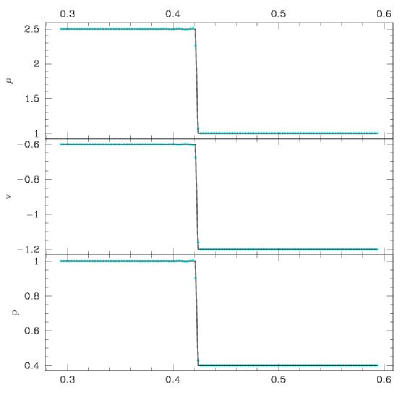
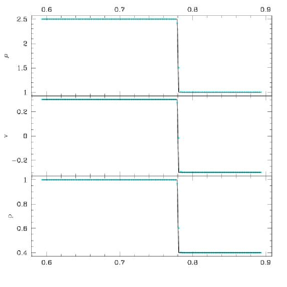
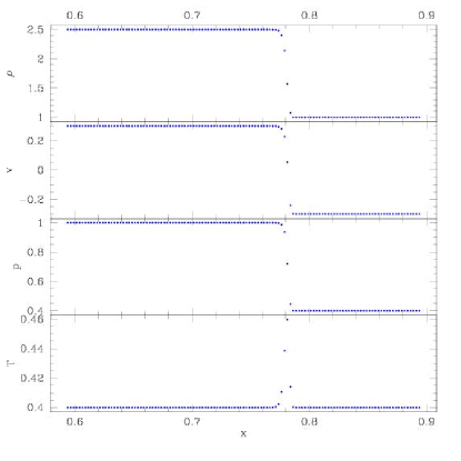
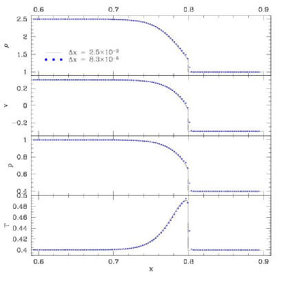
Next we study the case of an isothermal shock with initial conditions

$$\begin{array}[]{lll}\rho_{r}=1.0,&p_{r}=0.4,&u_{r}=u_{r}\\ \rho_{l}=2.5,&p_{l}=1.0,&u_{l}=u_{r}+0.6.\end{array}$$ (73)

The numerical results (solid dots) are shown together with the analytic solution (solid line) in Fig. 2 for two different values of $u_{r}$, namely $-1.2$ (top left) $-0.3$ (top right) producing isothermal shock fronts slowly moving to the left and the right, respectively. Neither artificial viscosity nor flattening was employed and a van Leer’s limiter was used. Overall the algorithm performs very well. The shock positions accord with the analytic value. The shocks are well captured within a couple of zones, indicating that the properties of the scheme have not degraded with respect to the non-stiff case. We notice that minor oscillations appear in a few zones downstream the left moving shock front. These have not been introduced by our method for treating the stiff source, but rather, are due to the fact that the dissipation in a Godunov method vanishes for slowly-left-moving shocks, such as the one being computed here. A thorough discussion on this is found in [20]. In particular, we find that the same oscillations appear in the purely hydrodynamic version of the algorithm with the relaxation term turned off, if we use an adiabatic index $0<\gamma-1\ll 1$ in order to mimic isothermality.

Finally, in the bottom right panel the same initial conditions as in the top right panel are used but in combination with a much smaller heat transfer coefficient, $K=500$ (bottom left) and $K=50$ (bottom right). In these cases $K^{-1}\leq\Delta x/c_{\rm eff}$ and $K^{-1}\geq\Delta x/c_{\rm eff}$, respectively, so that while the gas behavior is not strictly isothermal, the relaxation time is still relatively short. Assessing the algorithm performance for this situation is of relevance as well, as in general stiffness of the conditions will vary across a flow. The bottom panels of Fig. 2, in addition to density, velocity and pressure also present results for the temperature. As it appears from this plot, the numerical solution is very satisfactory, without numerical artifacts or oscillations. For the case $K=50$, we take the test one step further and compare the result obtained using the current grid settings (solid dots), that is $N_{cell}=400,~{}\Delta x=2.5\times 10^{-3}$, with those from a much higher resolution run (solid line) in which $N_{cell}=12000,~{}\Delta x=8.33\times 10^{-5}$ so that the reaction time is fully resolved. This comparison nicely shows that our modified scheme is able to capture the correct behavior of the flow even at intermediate stiffness conditions away from a purely isothermal behavior.

6.2 Convergence Rates in Smooth Flows

In this section we test the convergence of the method by studying the case of a smooth flow with the following initial conditions

$$\rho=\rho_{0}+\frac{{A}}{2}\left[\cos(2\pi\,{\bf k\cdot r})+1\right]$$ (74)

$$p=p_{0}=0.5$$ (75)

$$u_{x}=u_{x0}=0.3$$ (76)

$$u_{y}=u_{y0}=0.5$$ (77)

where ${\bf r}$ is the position vector and we use $\rho_{0}=\gamma=1.4$. The above initial conditions produce a sinusoidal wave with amplitude ${A}$ propagating in the domain along the direction defined by the vector ${\bf k}$. While we have experimented with various values for the parameters ${A}$, ${\bf k}$ and $K$, below we present results for a few cases only, summarized in Table 1.

Table 1: Run Set for Convergence Study with Relaxation Law Eq. (65)

run	${A}$	${\bf k}$	$K$	$\zeta$	$\eta$	Note
A	$10^{-2}$	$(1,0)$	$K=1$	0	0
B	$10^{-2}$	$(1,0)$	$K=50$	0	0
C	$10^{-2}$	$(1,0)$	$K=10^{8}$	0	0
D	$10^{-2}$	$(2/\sqrt{5},1/\sqrt{5})$	$K=1$	0	0
E	$10^{-2}$	$(2/\sqrt{5},1/\sqrt{5})$	$K=50$	0	0
F	$10^{-2}$	$(2/\sqrt{5},1/\sqrt{5})$	$K=10^{8}$	0	0
G	$10^{-2}$	$(1,0)$	$K=10^{8}$	0	0	$\delta e/e_{0}=0.4$
H	$10^{-2}$	$(2/\sqrt{5},1/\sqrt{5})$	$K=10^{8}$	0	0	$\delta e/e_{0}=0.4$
I	$10^{-2}$	$(1,0)$	$K=10^{8}$	1	0.1	$\delta e/e_{0}=0.4$
L	$10^{-2}$	$(2/\sqrt{5},1/\sqrt{5})$	$K=10^{8}$	1	0.1	$\delta e/e_{0}=0.4$

Table 2: Convergence Rates: 1-D Case: ${A}=10^{-2},~{}{\bf k}=(1,0)$

	density					momentum
$N_{\rm cell}$	$L_{1}$	$L_{2}$	$L_{\infty}$	$R_{1}^{\dagger}$		$L_{1}$	$L_{2}$	$L_{\infty}$	$R_{1}^{\dagger}$
	$K=1$
32	4.3E-7	9.5E-7	2.8E-6	–		6.3E-7	1.4E-7	4.0E-6	–
64	1.1E-7	2.4E-7	7.0E-7	2.0		1.3E-7	2.8E-7	8.0E-7	2.3
128	2.7E-8	6.0E-8	1.8E-7	2.0		2.8E-8	6.3E-8	1.8E-7	2.2
256	6.8E-9	1.5E-8	4.4E-8	2.0		6.7E-9	1.5E-8	4.2E-8	2.1
	$K=50$
32	4.0E-7	8.8E-7	2.6E-6	–		7.8E-7	1.7E-6	4.9E-6	–
64	1.1E-7	2.5E-7	7.2E-7	1.9		1.5E-7	3.2E-7	9.2E-7	2.4
128	3.1E-8	6.9E-8	2.0E-7	1.8		2.9E-8	6.5E-8	1.8E-8	2.4
256	8.5E-9	1.9E-8	5.4E-8	1.9		6.2E-9	1.4E-8	3.9E-8	2.2
	$K=10^{8}$
32	4.1E-7	9.2E-7	2.7E-6	–		8.2E-7	1.8E-6	5.91-6	–
64	9.7E-8	2.1E-7	6.4E-7	2.1		1.6E-7	3.6E-7	1.0E-6	2.4
128	2.3E-8	5.2E-8	1.5E-7	2.1		3.6E-8	8.0E-8	2.3E-7	2.1
256	5.7E-9	1.3E-8	3.8E-8	2.0		8.5E-9	1.9E-8	5.4E-8	2.1

^† $R_{1}$ is the convergence rate based on the $L_{1}$ errors.

In particular we consider a perturbation amplitude ${A}=10^{-2}$ and both a wave-vector aligned with the grid ${\bf k}=(1,0)$ and skew with respect to it, ${\bf k}=(2/\sqrt{5},1/\sqrt{5})$. We adopt a source term as given in Eq. (65) with values of the transfer coefficient $K=1,50,10^{8}$ to explore different regimes in which the relaxation is resolved in time, is stiff as well as the intermediate regime (cases A-F). We then repeat case C and F but with the initial value of the internal energy offset from the equilibrium value by $\delta e/e_{0}=40\%$ (cases G-H). Finally, we consider the case in which the source term depends both on density and internal energy, as described by Eq. (65). In particular, we show results concerning the case in which $K=10^{8}$, $\zeta=1$, $\eta=0.1$, $\delta e/e_{0}=40\%$ (cases I-L). Consistent test results were also found by setting $\zeta=1$, $\eta=0$ as well as $\zeta=0$, $\eta=0.1$.

In order to measure the rate at which the numerical solution converges, for each problem we carry out a set of 5 simulation runs employing $N_{cell}=32,64,128,256,512$ for a total range of 32. Note that the stiffness conditions do not change significantly as the grid is refined within the range of resolutions considered here. Also, the smallness of the perturbations is such that the term given by Eq. (64), to be added to the energy in the predictor step, is resolved in time

Table 3: Convergence Rates: 2-D Case: ${A}=10^{-2},~{}{\bf k}=(2/\sqrt{5},1/\sqrt{5})$

	density					momentum
$N_{\rm cell}$	$L_{1}$	$L_{2}$	$L_{\infty}$	$R_{1}^{\dagger}$		$L_{1}$	$L_{2}$	$L_{\infty}$	$R_{1}^{\dagger}$
	$K=1$
32	3.2E-5	3.5E-5	5.3E-5	–		4.3E-5	4.8E-5	7.0E-5	–
64	8.6E-6	9.5E-6	1.4E-5	1.9		9.8E-6	1.1E-5	1.6E-5	2.1
128	2.2E-6	2.5E-6	3.6E-6	2.0		2.3E-6	2.6E-6	3.8E-6	2.1
256	5.7E-7	6.4E-7	9.2E-7	2.0		5.7E-7	6.3E-7	9.1E-7	2.0
	$K=50$
32	6.2E-5	7.0E-5	1.0E-5	–		3.6E-5	4.0E-5	5.9E-5	–
64	1.2E-5	1.4E-5	2.0E-5	2.4		7.9E-6	8.8E-6	1.3E-5	2.4
128	2.7E-6	3.0E-6	4.3E-6	2.2		1.8E-6	1.9E-6	2.8E-6	2.1
256	6.2E-7	6.9E-7	1.0E-6	2.1		4.0E-7	4.5E-7	6.5E-6	2.2
	$K=10^{8}$
32	7.4E-5	8.2E-5	1.2E-4	–		4.5E-5	5.0E-5	7.3E-5	–
64	1.6E-5	1.8E-5	2.6E-5	2.2		1.0E-5	1.1E-5	1.7E-5	2.2
128	3.8E-6	4.2E-6	6.1E-6	2.1		2.5E-6	2.8E-6	4.1E-6	2.0
256	9.4E-7	1.0E-6	1.5E-6	2.0		6.2E-7	6.9E-7	9.9E-6	2.0

^† $R_{1}$ is the convergence rate based on the $L_{1}$ errors.

Table 4: Convergence Rates: Off Equilibrium Case: $\delta e/e_{0}=0.4$, ${A}=10^{-2}$, $K=10^{8}$

	density					momentum
$N_{\rm cell}$	$L_{1}$	$L_{2}$	$L_{\infty}$	$R_{1}^{\dagger}$		$L_{1}$	$L_{2}$	$L_{\infty}$	$R_{1}^{\dagger}$
	${\bf k}=(1,0)$
32	4.8E-7	1.1E-6	3.1E-6	–		7.6E-6	1.7E-6	4.8E-6	–
64	1.0E-7	2.3E-7	6.9E-7	2.2		1.5E-7	3.3E-7	9.5E-6	2.3
128	2.4E-8	5.4E-8	1.6E-7	2.1		3.3E-8	7.3E-7	2.1E-7	2.2
256	5.9E-8	1.3E-8	3.9E-7	2.0		7.7E-9	1.7E-8	5.9E-8	2.1
	${\bf k}=(2/\sqrt{5},1/\sqrt{5})$
32	7.4E-5	8.2E-5	1.2E-4	–		4.4E-5	4.9E-5	7.2E-5	–
64	1.6E-5	1.8E-6	1.7E-5	2.2		1.0E-5	1.1E-5	1.7E-5	2.1
128	3.8E-6	4.2E-6	6.2E-6	2.1		2.5E-6	2.8E-6	4.0E-6	2.0
256	9.4E-7	1.0E-6	1.5E-6	2.0		6.1E-7	6.8E-7	9.9E-7	2.0

^† $R_{1}$ is the convergence rate based on the $L_{1}$ errors.

Table 5: Convergence Rates: Off Equilibrium, $\rho$-dependent Source Case: $\delta e/e_{0}=0.4$, $\zeta=1$, $\eta=0.1$, ${A}=10^{-2}$, $K=10^{8}$

	density					momentum
$N_{\rm cell}$	$L_{1}$	$L_{2}$	$L_{\infty}$	$R_{1}^{\dagger}$		$L_{1}$	$L_{2}$	$L_{\infty}$	$R_{1}^{\dagger}$
	${\bf k}=(1,0)$
32	2.6E-7	5.7E-7	1.8E-6	–		9.0E-7	2.0E-6	5.7E-6	–
64	6.1E-8	1.4E-7	4.2E-7	2.1		1.9E-7	4.1E-7	1.2E-6	2.2
128	1.5E-8	3.3E-8	1.0E-7	2.0		4.2E-8	9.3E-8	2.7E-7	2.2
256	3.5E-9	7.7E-9	2.4E-8	2.1		1.0E-8	2.2E-8	6.5E-8	2.1
	${\bf k}=(2/\sqrt{5},1/\sqrt{5})$
32	6.6E-5	7.4E-5	1.1E-4	–		5.1E-5	5.7E-5	8.3E-5	–
64	1.5E-5	1.7E-5	2.5E-5	2.1		1.2E-5	1.3E-5	1.9E-5	2.1
128	3.7E-6	4.1E-6	5.9E-6	2.0		2.8E-6	3.1E-6	4.6E-6	2.1
256	9.1E-7	1.0E-6	1.5E-6	2.0		7.0E-7	7.7E-7	1.1E-6	2.0

^† $R_{1}$ is the convergence rate based on the $L_{1}$ errors.

The convergence rate is measured using Richardson extrapolation. Given the numerical result $q_{r}$ at a given resolution $r$ we first estimate the error at a given point $(i,j)$, as

$$\varepsilon_{r;i,j}=q_{r}(i,j)-\bar{q}_{r+1}(i,j)$$ (78)

where $\bar{q}_{r+1}$ is the solution at the next finer resolution, properly spatially averaged onto the coarser grid. We then take the n-norm of the error

$$L_{n}=\|\varepsilon_{r}\|_{n}=\left(\sum|\varepsilon_{r;i,j}v_{i,j}|^{n}\right)^{1/n}$$ (79)

where, $v_{i,j}=\Delta x^{2}$ is the cell volume, and estimate the convergence rate as

$$R_{n}=\frac{\ln(L_{n}(\varepsilon_{r})/L_{n}(\varepsilon_{s}))}{\ln(\Delta x_{r}/\Delta x_{s})}.$$ (80)

For each studied case listed Table 1, we produce a corresponding table (2-5) reporting the $L_{1},~{}L_{2}$ and $L_{\infty}$ norms of the error as defined above. Inspection of their values shows that the error drops with second order accuracy, supporting our analysis in Sec. 2..

A final experiment is designed to further prove that in the stiff limit ($K=10^{8}$) the proposed scheme converges to the correct asymptotic (isothermal) behavior. To do that we employ a Godunov method for the isothermal fluid equations and run again case C in Table 1. A comparison of the solutions obtained with the isothermal code and our proposed method is reported in Table 6. It shows that the difference between the two is always negligible with respect to the estimated truncation error, thus validating our convergence study.

Table 6: Comparison with a Purely Isothermal Solution: ${A}=10^{-2},~{}{\bf k}=(1,0)$

	density				momentum
$N_{\rm cell}$	$L_{1}$	$L_{2}$	$L_{\infty}$		$L_{1}$	$L_{2}$	$L_{\infty}$
32	2.7E-11	6.0E-11	1.7E-10		1.8E-10	4.0E-11	1.1E-10
128	2.7E-11	6.1E-11	1.7E-10		1.8E-10	4.0E-11	1.1E-10
256	2.7E-11	6.1E-11	1.7E-10		1.8E-10	4.0E-11	1.1E-10
512	2.7E-11	6.1E-11	1.7E-10		1.8E-10	4.0E-11	1.1E-10

6.3 Adaptive Mesh Refinement and Strong Shock Problems

In applications involving the interaction of strong shocks, it is useful to use the dissipation mechanisms described in [4], which generalize without modification to the present case. In addition, it is also desirable to couple this method to a block-structured adaptive mesh refinement (AMR) [1, 10]. In AMR calculations, the conservative variables are updated for the conservative fluxes in two steps. The first step constitutes the main flux update and it simply consists in modifying the state variables $U$ for the total fluxes across the cell boundaries. In addition, as part of the operations of synchronization among different levels, the conservative variables at the coarse-fine grid interfaces are further updated for the flux difference between the level on which they are defined and the next finer level. This operation is referred to as refluxing and it is aimed at preserving the conservative character of the numerical scheme when applied to a hierarchy of nested grids.

For the purpose of the current discussion, the effect of this operation can be expressed as

$$U\rightarrow U-\frac{\Delta t}{\Delta x}\delta F$$ (81)

where $\delta F$ is the difference between the fluxes at the coarse-fine interface computed on a given level and the next finer level. In AMR calculations refluxing on a given level is enforced as a separate operation, after the source update and the main flux update have been carried out on that level and also on all finer levels. Therefore, an additional measure must be taken to ensure that the effects of refluxing are also subjected to the action of the deferred corrections (just like the flux update does). Thus, inspection of Eq. (9)-(11) indicates that the flux correction must be modified according to

$$\delta F\rightarrow\left\{\left({\rm I}-\Delta t\nabla_{U}S|_{U_{0}}\right)^{-1}+\left({\rm I}-\Delta t\nabla_{U}S|_{\tilde{U}}\right)^{-1}\left[{\rm I}-\left({\rm I}-\Delta t\nabla_{U}S|_{U_{0}}\right)^{-1}\right]\right\}\,\delta F.$$ (82)

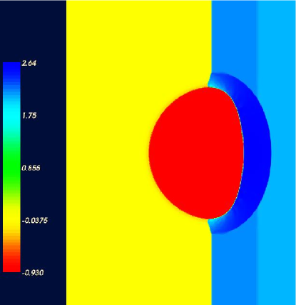
In the following we employ an AMR code and carry out a calculation involving the interaction of a spherical overdense region with a strong hydrodynamic shock to assess the robustness of our proposed numerical method. We assume a cloud overdensity with respect to the ambient medium $\chi=10$ and a shock Mach number ${\mathcal{M}}=10$.

Figure 3: Logarithmic pressure maps from the shock-cloud interaction run. The shock Mach number is 10 and the cloud overdensity is 10. The left panel shows the ‘isothermal’ case with $K=10^{8}$ and the right panel shows the case in which $K^{-1}\simeq\Delta x/v_{shock}$, i.e. the relaxation time is comparable to the shock cell crossing time. These calculations were performed with an AMR code which employed a base grid of 256$\times$256 zones and two additional levels of refinement with refinement ratio 2.

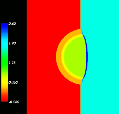
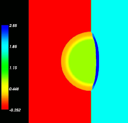
We use a base grid of 256$\times$256 zones and allow for two additional levels of refinement with refinement ratio 2 in regions where the undivided, relative density gradients, $\Delta\rho/\rho$, exceed 20%.

We begin assuming that a stiff relaxation term of the form in Eq. (65) acts on the flow internal energy and we consider both the case of a exceedingly large transfer coefficient, $K=10^{8}$, as well as the case in which the relaxation time is comparable to the shock cell crossing time. This requires, roughly, that

$$K^{-1}\simeq\Delta x/u_{shock}$$ (83)

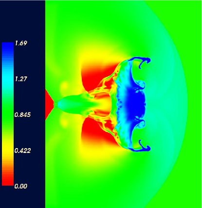
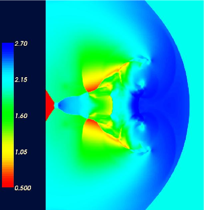
where $\Delta x$ is the mesh size and $u_{shock}$ is the shock speed. Note that the stiffness is sufficiently large that refining by a factor of 2 or 4 does not make the problem significantly less stiff. At simulation start the temperature is constant throughout the domain, so that the cloud is in thermal equilibrium but it has higher pressure than its surroundings. As a result, it expands sonically into the background. The shock propagates from the right to the left along the x-axis and as it runs into the cloud it crushes it. In Fig. 3 we plot the logarithmic pressure map as the shock is roughly half-way through the cloud. The high pressure postshock region is clearly thinner in the case of the larger value of $K$ and the shock has also propagated slightly further down the axis. In both cases, however, the result is sound and shows no sign of numerical artifact both in the presence of strong shock and large gradients, and independently of the magnitude of the transfer coefficient.

Figure 4: Logarithmic density (left) and pressure (right) maps from the shock-cloud interaction run for a density dependent source term at $t=0.018$ (top) and $t=0.07$ (bottom) time units. As before, the shock Mach number is 10, the cloud overdensity is 10 and the calculation was performed with an AMR code employing a base grid of 256$\times$256 zones and two additional levels of refinement with refinement ratio 2.

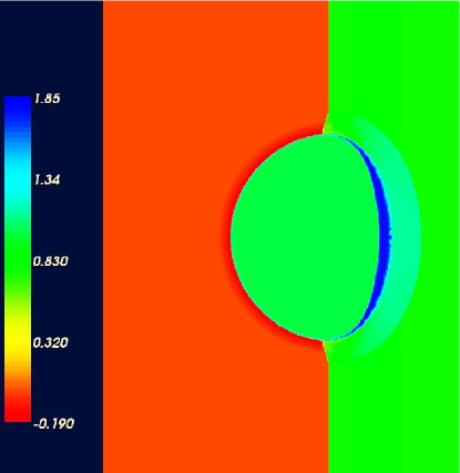
As a final test, we consider the same shock cloud interaction problem as described above but with a source function appropriate for a mixture of hydrogen (76 %) and helium (24 %) illuminated by a uniform ionizing background radiation field. The cooling part of the source function is proportional to the density and the equilibrium temperature, of order $10^{4}$ K, depends slightly on the density. This function has a very strong temperature gradient about the equilibrium value, behaving analogously to the stiff source terms used in the previous sections were accuracy and convergence studies were carried out.

We set the background gas temperature to $10^{6}$ K and its number density to 0.1 cm^-3. The gas is collisionally ionized, its sound speed is of order $1.2\times 10^{7}$ cm s^-1 and it has a cooling time $\tau_{cool}=P/(\gamma-1)\rho\Lambda\simeq 1.4\times 10^{7}$ yr. With a box size $L=1.7$ kpc = $5.2\times 10^{21}$ cm, the latter is much longer than the CFL time, $\tau_{CFL}\leq\Delta x/u_{shock}\simeq 5.4\times 10^{3}$ yr. The cloud of overdense gas is in pressure equilibrium with a density contrast $\chi=10$ so that its temperature is $10^{5}$ K. When unperturbed, the cloud’s gas cooling time is about $1.4\times 10^{4}$ yr $\simeq 2.6\times\tau_{CFL}$. A background radiation field, producing about $\Gamma\sim 2.4\times 10^{-12}$ s^-1 ionizations of neutral atoms of hydrogen and helium keeps the cloud’s temperature at the equilibrium value of $\sim 1.510^{4}$ K. However, the cloud’s pressure quickly falls below the background value and, as a minor effect, the cloud slowly contracts.

Fig. 4, shows a snapshot of the density (left) and the pressure (right) during the initial (top) and final stages (bottom) of the simulation. The reverse shock is non-radiative, thus extending further ahead of the cloud than in the previous cases in Fig. 3. Inside the cloud strong radiative losses prevent the full temperature rise in the postshock region and produce a density jump substantially larger than in the corresponding adiabatic case. The bottom panel shows the later stages of the cloud evolution, when Rayleigh-Taylor instability with scales comparable to the cloud size have developed and are shredding the cloud. As in the previous case, in which the source term is described by a relaxation law, the code appears to produce reliable numerical results, without numerical artifact despite the presence of strong shock and large gradients.

7 Conclusions

We have presented a second order accurate semi-implicit predictor-corrector scheme to treat stiff source terms within the framework of higher order Godunov’s methods. Our treatment of the predictor step for computing the hyperbolic fluxes, is based on the derivation of a local effective dynamics using Duhamel’s formula. This leads to a conventional second-order Godunov method when the system relaxation time is larger than the time step and to a second-order Godunov method for the isothermal equations in the limit of a stiff source term. Finally, we obtain a semi implicit corrector using a one-step second-order accurate deferred corrections method as suggested in [5, 12].

Our tests indicate that the proposed method is stable, robust and its second order accuracy preserved across a variety of stiffness conditions. We have also discussed the case of a general source term which depends both on $e$ and $\rho$ and shown that the method is applicable provided that the flow is thermally stable or the non-stiff part of the source term is resolved in time.

The additional cost involved in the formulation of our scheme is minimal; all it requires is an estimate of the term $\Lambda_{e}$ which in a purely relaxation case is trivial and for a more complicated source term (such as the case of radiative losses) is still minor compared to the estimate of the source term itself. In our implementation the factor $\alpha(\gamma-1)+1$ is stored as an additional primitive variable and used as polytropic index in the characteristic analysis in stead of $\gamma$.

Acknowledgment

FM is grateful to the Lawrence Berkeley National Laboratory for its hospitality and acknowledges support by the Swiss Institute of Technology through a Zwicky Prize Fellowship. PC was supported by the Mathematical, Information, and Computing Sciences Division of the United States Department of Energy Office of Science under contract number DE-AC02-05CH11231.

References

- [1] M. J. Berger and P. Colella. Local adaptive mesh refinement for shock hydrodynamics. Journal of Computational Physics, 82:64–84, 1989.
- [2] R. E. Caflisch, S. Jin, and G. Russo. Uniformly accurate schemes for hyperbolic systems with relaxation. SIAM J. Sci. Comput., 34(1):246–281, 1997.
- [3] G. Q. Chen, C. Levermore, and T. Liu. Hyperbolic conservation laws with stiff relaxation terms and entropy. Comm. Pure Appl. Math., 47:787–830, 1994.
- [4] P. Colella. Multidimensional upwind methods for hyperbolic conservation laws. Journal of Computational Physics, 82:64–84, 1989.
- [5] A. Dutt, L. Greengard, and V. Rokhlin. Spectral deferred correction methods for ordinary differential equations. BIT, 40:241–266, 2000.
- [6] G. B. Field. Thermal instability. Astrophys. Journal, 142:531, 1965.
- [7] S. Jin. Runge-kutta methods for hyperbolic conservation laws with stiff relaxation terms. J. Comput. Phys., 122:51–67, 1995.
- [8] S. Jin and D. Levermore. Numerical schemes for hyperbolic conservation laws with stiff relaxation terms. J. Comput. Phys., 126:449–467, 1996.
- [9] S. Jin, L. Pareschi, and G. Toscani. Diffusive relaxation schemes for multiscale discrete-velocity kinetic equations. SIAM J. Sci. Comput., 35(6):2406–2439, 1998.
- [10] F. Miniati and P. Colella. Block structured adaptive mesh and time refinement for hybrid, hyperbolic + n-body systems. Journal of Computational Physics, 2006. submitted.
- [11] F. Miniati, D. Ryu, H. Kang, T. W. Jones, R. Cen, and J. Ostriker. Properties of cosmic shock waves in large-scale structure formation. Astrophys. Journal, 542:608–621, 2000.
- [12] M. Minion. Semi-implicit spectral deferred correction methods for ordinary differential equations. Comm. Math. Sci., 1:471–500, 2003.
- [13] L. Pareschi and G. Russo. Implicit—explicit runge—kutta schemes and applications to hyperbolic systems with relaxation. SIAM J. Sci. Comput., 25(1):129–155, 2005.
- [14] R. B. Pember. Numerical methods for hyperbolic conservation laws with stiff relaxation ii: higher-order godunov methods. SIAM J. Sci. Comput., 14(4):824–859, 1993.
- [15] P. L. Roe and A. F. Hittinger. Toward Godunov-type methods for hyperbolic conservation laws with stiff relaxation. In E. F. Toro, editor, Godunov Methods: Theory and Applications, pages 725–744, New York, 2001. Kluwer Academic/Plenum Publishers.
- [16] J. Saltzman. An Unsplit 3D Upwind Method for Hyperbolic Conservation Laws. Journal of Computational Physics, 115:153–168, November 1994.
- [17] D. Trebotich, P. Colella, and G. H. Miller. A stable and convergent scheme for viscoelastic flow in contraction channels. Journal of Computational Physics, 205:315–342, May 2005.
- [18] W. G. Vincenti and C. H. Kruger. Introduction to Physical Gas Dynamics. John Wiley, New York, 1965.
- [19] G. B. Withman. Linear and Non-Linear Waves. Wiley-Interscience, New York, 1974.
- [20] P. R. Woodward and P. Colella. Numerical simulations of two-dimensional fluid flow with strong shocks. Journal of Computational Physics, 54:115–173, 1984.