Smear fitting: a new image deconvolution method for interferometric data

Abstract

A new technique is presented for producing images from interferometric data. The method, “smear fitting”, makes the constraints necessary for interferometric imaging double as a model, with uncertainties, of the sky brightness distribution. It does this by modelling the sky with a set of functions and then convolving each component with its own elliptical gaussian to account for the uncertainty in its shape and location that arises from noise. This yields much sharper resolution than CLEAN for significantly detected features, without sacrificing any sensitivity. Using appropriate functional forms for the components provides both a scientifically interesting model and imaging constraints that tend to be better than those used by traditional deconvolution methods. This allows it to avoid the most serious problems that limit the imaging quality of those methods. Comparisons of smear fitting to CLEAN and maximum entropy are given, using both real and simulated observations. It is also shown that the famous Rayleigh criterion (resolution = wavelength / baseline) is inappropriate for interferometers as it does not consider the reliability of the measurements.

1 Introduction

Interferometers give us a much sharper view than filled aperture telescopes of the same area, by sampling the sky’s spatial frequencies with a set of baselines given by the separations between each receiver. Unfortunately the distribution of samples (“visibilities”) is incomplete, so the Fourier transform of the measured visibilities is not the sky brightness distribution. The Fourier transform of the visibilities instead yields the “dirty map”, which is the sky brightness distribution plus noise, convolved with the dirty beam (the Fourier transform of the sampling pattern). In other terms, a simple Fourier transform produces an image with absolutely no power at unsampled spatial frequencies. As a result the dirty beam exhibits sidelobes causing the fainter structure in the image to be buried under the diffraction patterns of the brightest objects in the field.

Unfortunately the most straightforward way of deconvolving away the effect of the dirty beam would divide by zero in the $uv$ plane (the Fourier transform of the image plane) wherever no measurement was made, and practical methods must instead attempt to fill unmeasured regions of the $uv$ plane with a more reasonable estimate than zero. Simply interpolating between the visibilities does not work in general because aliasing of oscillations in the $uv$ plane can erroneously move the emission toward the center of the image plane, and distort its appearance. Thus there is no unique prescription for extracting the optimum estimate of the true sky brightness, and many methods, most notably CLEAN (Högbom, 1974) and maximum entropy deconvolution (Gull & Skilling 1983, Cornwell et al. 1999), that vary in their properties have been devised. They are usually, if not strictly correctly, called deconvolution methods. They rely on expected or desired properties of the images such as positivity, locality, or smoothness to constrain the images they produce. This paper presents a new method, called smear fitting, which uses as simple a model as it can as its main constraint, and can optionally use additional constraints such as positivity and/or confinement of the source to a certain region. It renders the measurements into images with better fidelity and resolution, and fewer image artifacts, than traditional deconvolution methods.

A great benefit of smear fitting is considerably improved resolution for objects with peak brightness greater than 4.20 times the root mean square (rms) noise (it does not change the resolution of fainter features) without a loss of sensitivity from reweighting the data. This feature is extremely important since better resolution cannot be achieved by simply adding data, and the noise that comes with it, from longer baselines or decreasing the weight of short baselines, without increasing the root mean square (rms) errors in surface brightness over the whole image. The objects of interest in typical radio astronomical observations span wide ranges of both brightness and size, and smear fitting offers a way to optimally handle both. Smear fitting also produces a set of components modelling the source, and calculates the uncertainties of the distribution of those components on the sky. The components often correspond to distinct physical features of the source(s), making their parameters and associated uncertainties of immediate scientific interest.

Smear fitting has been implemented as a modification (patch) to difmap (Shepherd, 1997). The patch, known as smerf, is freely available at http:$/\!$/www.drao-ofr.hia-iha.nrc-cnrc.gc.ca/$\!\sim$rreid/smerf/.

2 Smear Fitting

2.1 Procedure

Smear fitting is a two step process. In the first step a set of components, usually elliptical gaussians, with total visibility function ${\sf V}_{\mbox{\it\scriptsize model}}(u,v;\vec{p})$ is fitted to the visibilities ${\sf V}_{i}$ by varying the parameters $\vec{p}$ to minimize $\chi^{2}$:

$$\mbox{$\chi^{2}$}=\sum_{i}\left|\frac{{\sf V}_{i}-{\sf V}_{\mbox{\it\scriptsize model}}(u_{i},v_{i};\vec{p})}{\sigma_{i}}\right|^{2}$$ (1)

where $\sigma_{i}$ is the uncertainty of measurement ${\sf V}_{i}$. In the second step each component is broadened, or “smeared”, until $\chi^{2}$ is raised by the number of degrees of freedom of the component’s distribution on the sky. The visibility model and residuals are then Fourier transformed and summed together to form an image. An example of the effect of smearing is shown in Figure 1.

The goal of this process is a final map that shows what viewers intuitively expect when looking at an image with resolution known to be imperfect: the true image convolved by the probability distribution of where the radiation originates from. The smeared map is ideally equivalent to the average of an ensemble of maps produced from all possible realizations of the noise added to the measured visibilities. The first implementation of smear fitting used the Monte Carlo method, but the current technique of broadening the components until $\chi^{2}$ is raised by a certain amount is far more efficient.

In the first step, producing an unsmeared model, it is usually impossible to specify a model in its entirety and then simultaneously fit all of its parameters. This is because typical initial dirty maps are dominated by a small number of bright objects that must be modeled and removed before the underlying structure becomes apparent, exactly as with CLEAN. Fortunately components that do not appreciably overlap can be independently fitted, as can neighboring features with proper downweighting of the short baselines (Reid, 2003). Therefore the model is built incrementally (either manually or by running a script) with cycles of:

1. Adding to the model one or more elliptical gaussian(s) for the brightest peak(s),

2. specifying the set of parameters that should be fitted (which includes parameters from previously fitted components that will be affected by the new component(s)), then

3. fitting them to the visibilities by minimizing $\chi^{2}$.

A gaussian component fit to an unresolved source can approach a $\delta$ function, naïvely extrapolating power to spatial frequencies far beyond those sampled by the measurements. This makes it necessary to somehow smooth the model so that it does not claim a higher resolution than the measurements warrant. Smear fitting accomplishes that with its second step, “smearing”. During smearing, each component of the model is broadened by minimizing the sharpness function while constraining $\chi^{2}$ to rise to $\chi^{2}_{\textit{{\scriptsize unsmeared}}}+\Delta$ using a Lagrange multiplier. The sharpness function is

$$B=\frac{2\pi}{u_{\textit{\scriptsize max}}^{2}}\frac{\sum_{c}f_{c}^{2}/A_{c}}{\sum_{c}f_{c}^{2}}$$ (2)

where $f_{c}$ and $A_{c}$ respectively are the flux and effective area of a component $c$. The effective area of a gaussian is $2\pi r\sigma^{2}=\pi ra^{2}/(4\ln 2)$, where $r$ is its (minor/major) axial ratio and $\sigma$ and $a$ are its standard deviation and full width at half maximum (FWHM) along its major axis. Only relative changes in $B$ matter, so it is convienient to scale it using $u_{\textit{\scriptsize max}}$, the maximum baseline length in wavelengths. That makes the contribution to $B>1$ for components sharper than the spatial frequency corresponding to the longest baseline. Squaring the fluxes allows $B$ to be used with negative components as well as positive ones.

The form of $B$ came from devising a function to measure the squared amplitude of the model visibilities integrated over the entire $uv$ plane relative to the squared total flux, with a modification to ignore component overlaps. The larger $B$ is, the more of the model is in the part of the $uv$ plane unsupported by measurements, so it is a quantity that should be minimized by reliable models. Each component’s flux is held fixed during smearing to prevent the sharpness decreasing by transferring flux between unrelated components.

$\Delta$ is a positive number limiting the amount of smearing that is allowed. The larger it is, the more smearing there will be, corresponding to a larger confidence region of the model parameters. Although model parameters are often reported with confidence intervals of $\pm 2$, 3, or more standard deviations, in the presentation of an image it is most natural to plot the image “smeared by one standard deviation” in order to recreate the probability distribution of the emission on the sky. Another reason to only use one standard deviation is that it is customary in radio interferometry to publish images with whatever is not accounted for by the deconvolution (the residuals) added to the result of the deconvolution. Since smearing reduces the amplitude of the long baseline model visibilities (broadening the image plane distribution makes the $uv$ plane distribution more compact), it effectively returns information from the model to the residuals. The residual map is of course dirty, so the final map will appear “dirtier” wherever the effective smearing beam is comparable to or larger than the dirty beam. This is most likely not the desired effect, so it is important to distinguish performing a reliable deconvolution of a set of data from displaying only the information in that data that meets a certain level of reliability. The former is what smear fitting tries to do, but it can be adapted to the latter task by displaying only the model in the final image, setting $\Delta$ appropriately, and making it clear that the resulting image is almost certainly missing some real structure that did not “make the cut”.

Finding $\Delta$ for a given confidence level is accomplished by considering the Monte Carlo view of the process and requiring that the fraction of models with $\chi^{2}$ no greater than $\chi_{\textit{\scriptsize orig}}^{2}+\Delta$, after being perturbed by noise and refit, matches the confidence level. Assuming gaussian errors in the data, the model parameters will lie within $\pm 1$ standard deviation of the best fit 68.3% of the time. Typically each component is an elliptical gaussian smeared on its own, so the relevant degrees of freedom in its distribution on the sky are its location (2 degrees), major axis, axial ratio, and position angle, for a total of 5 degrees of freedom. Solving

$$0.683=\int_{0}^{\Delta}P_{5}(\mbox{$\chi^{2}$})d\mbox{$\chi^{2}$}$$ (3)

with $P_{5}(\mbox{$\chi^{2}$})$ being the probability distribution for $\chi^{2}$, yields $\Delta=5.89$. $\Delta$ for a 2 $\sigma$ confidence interval with 5 degrees of freedom comes from solving

$$0.954=\int_{0}^{\Delta}P_{5}(\mbox{$\chi^{2}$})d\mbox{$\chi^{2}$}$$ (4)

and is 11.3.

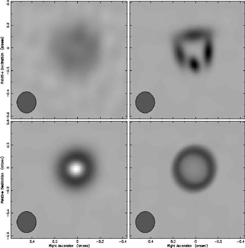
To maintain the relation between convolving each feature with its uncertainty and minimizing the sharpness while raising $\chi^{2}$ by $\Delta$, it is usually necessary to smear each component separately. Otherwise a bright sharp component would steal the portion of $\Delta$ that would normally go to a fainter, broader, component, even if they were unrelated. The only justification for simultaneously smearing more than one component is when the components are inseparable parts of a single feature. In such (rare) cases some customization is needed, either a modification of the sharpness function to fairly distribute the smearing, or preferably replacement of the generic elliptical gaussian components with a single component of a different type. Currently implemented alternatives to elliptical gaussian components are uniformly bright (i.e. optically thick) elliptical disks, optically thin ellipsoids (Figure 2), and Sunyaev-Zel’dovich clusters (Pearson, 1999, p. 351).

Figure 1: Before and after smearing compared to CLEAN for a naturally weighted VLA snapshot observation of J0354–052 (Reid et al., 1999). Top left: unsmeared image. Top right: smeared image. Note that smearing fattens the knife-edges, and that less significant components (shown as ellipses with FWHM major and minor axes) are smeared more. Bottom left: unsmeared image convolved with the CLEAN beam. Bottom right: CLEAN image. The contours start at 0.125 mJy/arcsec² and are each separated by a factor of 2. The solid gray ellipse in the lower left corner of each image is the FWHM CLEAN beam.

Figure 2: A young planetary nebula, Vy2-2, as it appeared at 15 GHz in February 1982. Top left: uniformly weighted CLEAN. Top right: The result of automatic smear fitting with the modcons script. Bottom left: the result of fitting and then simultaneously smearing a positive and a negative gaussian. Note the negative intensity in the center of the shell. Bottom right: the result of fitting and then simultaneously smearing a positive and a negative optically thin ellipsoid (OTE). Vy2-2 is expected to be an optically thin shell, and it appears to be well modeled by the nested OTEs. The grayscale is a linear ramp from $-1.725$ (white) to 3.510 (black) Jy/arcsec², and the flat gray ellipses are the FWHM beam extents.

2.2 The expected amount of smearing

A rule of thumb for the amount of smearing an isolated component will receive can be generated using the following approximations:

1. The $uv$ sampling density is taken to be an elliptical gaussian, specifically the Fourier transform of the CLEAN beam.

2. Smearing is restricted to convolving the unsmeared component with a scaled version of the CLEAN beam with major axis $k$ times as large as the CLEAN beam’s major axis, $a_{b}$.

3. The component’s unsmeared shape is assumed to have the same axial ratio and position angle as the CLEAN beam, so that it can be specified by the single parameter $\zeta\equiv a_{c}/a_{b}$, where $a_{c}$ is the component’s major axis.

Then the expected rise in $\chi^{2}$ due to smearing is

$$\left<\Delta\mbox{$\chi^{2}$}\right> = \frac{2f_{c}^{2}W}{1+2\zeta^{2}}\frac{\xi^{2}}{1+3\xi+2\xi^{2}},$$ (5)

$$\mathrm{with}\ \xi \equiv \frac{k^{2}}{1+2\zeta^{2}}$$ (6)

and $W$ being the sum of the visibility weights.

According to Equation 5, $\left<\Delta\mbox{$\chi^{2}$}\right>$ asymptotically approaches a maximum of $f_{c}^{2}W/(1+2\zeta^{2})^{2}$ for large smearing beams. This means that sufficiently diffuse components do not possess enough signal to reach the target $\left<\Delta\mbox{$\chi^{2}$}\right>$ of $\Delta$, due to a combination of insufficient flux and the fact that as components are broadened they affect fewer visibilities. Using the above approximations, the limit at which smearing to a level of $\Delta$ cannot be done is

$$f_{c}^{2}W\simeq(1+2\zeta^{2})\Delta$$ (7)

For a component that is unresolved in the unsmeared map, this corresponds to a surface brightness of $\sqrt{\Delta}$ times the theoretical r.m.s. noise of the image. If the component is significantly resolved, the surface brightness threshold approaches $\sqrt{2\Delta}$ times the rms level. In other words, there is, unsurprisingly, a minimum surface brightness required for the location and shape of a component to be determinable with any significance. This holds true even when the above approximations are relaxed.

Thus a low surface brightness component can be completely smeared away without sufficiently raising $\chi^{2}$. In effect, it is completely returned to the residual map, and should be removed to simplify the model. If it contains a significant amount of flux it should be CLEANed, since the dirty beam has no total flux unless single dish measurements have been included.

2.3 Instabilities in model construction and techniques to overcome them

Most radio observations have objects in their field that are too compact to be resolved with the given data, and as $\chi^{2}$ is minimized, there is little to stop the major and minor axes of the model components corresponding to those objects from collapsing to zero. Presumably all true sources have a nonzero size, but the noise, since most of it originates in the $uv$ plane instead of on the sky, does not necessarily obey the same rules as physical sources. The noise amplitude does not decrease with increasing baseline length (worse, it gains weight since the visibilities become more isolated), so it is quite easy for noise to collapse a compact component’s shape (see the appendix). When that happens the best thing to do is to fix the minor (and major, if necessary) axes at tiny but nonzero values and to move on to other components. This has no effect on the final image since the width of the smeared component will be dominated by its smearing “beam”.

The “knife-edge” case of a component with an extended major axis but collapsed minor axis is particularly common since it does not require a conspiracy of noise on both axes, and there are additional ways to produce it. The original version of difmap featured an interesting shape parameterization that unfortunately allowed the fit to enter a domain where the minor axis was imaginary. Once that happened the minor had to be clamped at zero and it became very difficult for the fit to return to physical plausibility. The smerf patch to difmap features a better shape parameterization (Equations 8 and 9) that allows the model fitting routine to try any real value for the internal parameters $\alpha$ and $\gamma$ while keeping the full width half maximum of the major axis, $a_{\mbox{{\it\scriptsize{maj}}}}$, and axial ratio $r$ (ratio of the minor axis to the major axis), within their physically allowable domains:

$$a_{\mbox{{\it\scriptsize{maj}}}} = \frac{e^{\alpha}}{\pi u_{\mbox{{\it\scriptsize{max}}}}}$$ (8)

$$r = (\gamma^{2}+1)^{-1}$$ (9)

$u_{\mbox{{\it\scriptsize{max}}}}$ is the longest baseline length.

Also, knife-edges can appear where one model component has been used to fit two unresolved features on the sky, so that $\chi^{2}$ minimization joined the features with a line. smerf can automatically detect and remove such knife-edge components, replace them with pairs of smaller components (if they are sufficiently far apart), and reminimize $\chi^{2}$.

All of the above issues occur in the venerable model fitting stage of smear fitting, and have fostered an impression in the community that fitting large sets of elliptical gaussians to interferometer data is not feasible. smerf includes several features to improve the robustness of model fitting, but truly unresolved sources are ubiquitous, and smerf’s main method of dealing with them is smearing. Smearing broadens each component as much as possible given the constraints of the data, smoothing $\delta$ functions and knife-edges as in Figure 1, and at the same time adds to the image a probability distribution for the locus of each component. The smeared map provides a very intuitive way to judge whether different components correspond to significantly distinct features on the sky.

3 Comparison To Established Methods

3.1 CLEAN

The CLEAN process (Högbom 1974 and Cornwell et al. 1999) is similar to smear fitting except that it uses $\delta$ functions for the components and a fixed gaussian for “smearing”, which is called restoration in the CLEAN nomenclature. Most of the difference between the two methods in the final image arises from the choice of smearing beam, but the philosophical difference between the methods is in the way they interpolate between visibilities in the $uv$ plane. Smear fitting tries to make a gaussian go through the error bars of each visibility, but CLEAN fits the flux in the central visibilities and tapers off its gaussian according to the sampling density (Figure 4), even though the sky distribution is unaffected by the sampling density. In other words, CLEAN fails to fit the measurements and tends to underestimate the achievable resolution.

Smearing convolves faint components with a (potentially much) larger beam than CLEAN. Using Equation 5 and its accompanying approximations, the threshold at which the smearing beam becomes larger than the CLEAN beam (Figure 3) is

$$\frac{I}{I_{\textit{\scriptsize rms}}}\simeq\left[(1+2\zeta^{2})(3+5\zeta^{2}+2\zeta^{4})\Delta\right]^{1/2}/(1+\zeta^{2})$$ (10)

For a component that is unresolved in the unsmeared map, this corresponds to a surface brightness of $\sqrt{3\Delta}$ times the theoretical root mean square noise of the dirty image. For unresolved elliptical gaussians smeared by one standard deviation, smearing is effectively equivalent to CLEAN at approximately $\sqrt{3\Delta}\ (\simeq 4.20)$ times the rms surface brightness. If the component is significantly resolved ($\zeta\rightarrow\infty$), the threshold surface brightness ratio quickly approaches $2\zeta\sqrt{\Delta}\ (\simeq 4.85\zeta)$. The smearing beam continues to enlarge below that threshhold, becoming infinitely large as the surface brightness of the unsmeared feature approaches zero.

Figure 3: The surface brightness limit (relative to the theoretical root mean square noise) in the dirty map at which the smearing beam (one standard deviation) would be same size as the CLEAN beam for an elliptical gaussian, as a function of $\zeta$, the ratio of the unsmeared component major axis $a_{c}$ relative to the CLEAN beam major axis $a_{b}$.

Technically, this means that CLEAN is placing too much faith in the sharpness and/or positional accuracy of the measurements for components below the surface brightness limit in Equation 10, but in imaging terms smear fitting’s behavior is very similar in the normal case, where the residuals are added to the model for the final image. When a component is severely smeared, its model only accounts for the innermost visibilities, and leaves the outer baselines in their original form. In other words, the more a component is smeared, the more the dirty beam shows through in the final image, and the appearance of a radically smeared component in the final image is not really broadened any more than it would be by CLEAN. The size of the smearing beam for each component can still be seen however, in a textual listing of the smeared model.

3.1.1 Total Flux Density and Source Counts

Although there is little cosmetic benefit to adding features below the limit of Equation 10 to the model, it can be useful for both CLEAN and smear fitting when the total flux density in the field is of interest, but no zero baseline (i.e. single antenna) measurement is readily available. In that common case, the theoretical total flux density in the dirty beam, and thus the residual map, is zero. Practically, the positive part of the dirty beam is concentrated in the central lobe and the negative part is spread over the rest of the Fourier transformed region, so a sum of the residuals over a small area will have nonzero flux density. A more accurate estimate of the total flux density can be obtained by modelling the trend of the short baseline visibilities using a deconvolution method and including diffuse structure that would not otherwise require deconvolution. Both CLEAN and smear fitting can include arbitrarily faint components in their models although systematic effects can make those components unreliable.

As with CLEAN, a source count will of course be incomplete if model construction is stopped early and only the component list (instead of the image) is used for the count. Similarly to flux estimation, either the model construction stage of smear fitting can be continued to the required depth, or a different deconvolution method may be used for the fainter emission. More interestingly, a single smear fitted component can correspond to many CLEAN components, so a list of smear fitted components should provide a more accurate raw count than a list of CLEAN components to the same depth. More accuracy, however, does not imply absolute accuracy. Typically, but not always, smear fitting allocates one component for each resolved feature, and the counter still needs to decide which components should be coalesced into “sources”.

3.1.2 Visibility weighting

Since CLEAN depends so heavily on the sampling pattern, it is customary to weight the outer visibilities more heavily than the inner ones, sacrificing some sensitivity (especially to diffuse objects) for an improvement in resolution (Briggs, 1995). The basic idea of a common procedure, called uniform weighting, is to weight each visibility by the reciprocal of the number of visibilities within a certain distance of it. Since long baselines tend to be more isolated than short ones, uniform weighting – or anything more extreme, called superuniform weighting – produces more compact central lobes in the dirty beam, but the rms noise in the surface brightness is degraded by the partial removal of short baseline data and the decrease in beam area (the rms noise in the surface brightness is inversely proportional to the product of the beam area and the square root of the number of measurements).

Smear fitting does not require any reweighting in its final images, and dynamically allocates the outer visibilities as much control as they deserve based on their signal to noise ratios, so it achieves optimum sensitivity without sacrificing any resolving power.

3.1.3 Fixed vs. variable resolution

Smear fitting can, unlike CLEAN, adapt to scales smaller than the dirty beam without losing sensitivity to diffuse structure (Figures 6, 10, and 11). In fact the most striking difference between smear fitted images and CLEAN images is that smear fitted images usually include one or more peaks that are much sharper than the dirty beam. It has been a long held precept that the smallest resolvable angle, $\theta_{\textit{\scriptsize min}}$, is given by $\theta_{\textit{\scriptsize min}}=1.2\lambda/D$, where $D$ is the effective diameter of the telescope. That equation comes from the Rayleigh criterion for a circular aperture (Born & Wolf, 1999), which states that two equally bright point sources are indistinguishable from a single source if their separation is less than the distance between the diffraction pattern’s central peak and its first minimum, since at that distance most diffraction pattern convolved features appear to meld together. Deconvolution methods that reveal details finer than the diffraction pattern are thus often called “superresolving”, but since the purpose of deconvolution is to remove the effect of the diffraction pattern, the Rayleigh criterion is not the right one to use as a standard for resolution.

In general the achievable resolving power of deconvolution is limited by how well the effect of the diffraction pattern can be removed, which is determined by both the size of the diffraction pattern’s main lobe and the signal to noise ratios of the features to be resolved. The blended beams of very close features are difficult to disentangle unless the data have a high signal to noise ratio, and conversely distant features are not reliably separated if one or both are so faint that the probability distributions of their locations significantly overlap.

Figure 4: The response in the $uv$ plane of smear fitting, CLEAN, and maximum entropy to a simulated snapshot observation (error bars) of a 10 mJy point source (horizontal gray line) by a 7 antenna VLA subarray. Maximum entropy did not perform well with this extremely sparse set of data, and unlike the other deconvolutions did not have the beneficial constraint of fitting a very simple model to this very simple source. Also, its prior (a flat image) was completely inappropriate for a point source, so this should not be considered to be a typical case for maximum entropy deconvolution.

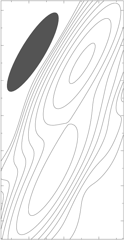
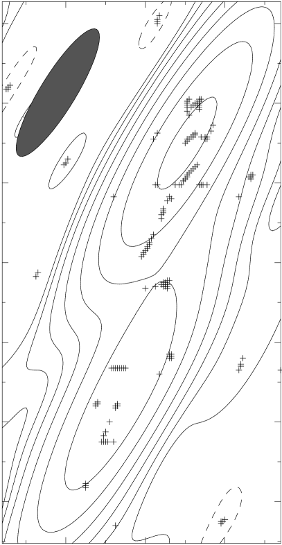
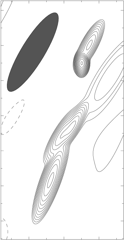
As illustrated in Figure 4, the resolution of the CLEAN beam (and the Rayleigh criterion) is set by the average spatial frequency of the measurements regardless of their values. That is exactly what is needed to emulate a nondeconvolved image from a filled aperture telescope of the same size, since with filled aperture instruments there is one detector per direction (for example, a pixel in a CCD) that simply receives the sum of all the spatial frequencies sampled by the dish. Interferometers have separate measurements of the visibility function at the sampled spatial frequencies, which the model fitting step of smear fitting uses to discern the trend of the data. The smearing step biases the model within the framework of its parameters to be as broad as possible without deviating too far from the data. Figure 5 demonstrates that CLEAN is able to detect sub-beamwidth structure which is obliterated by the restoring beam in the final image. Smear fitting is able to display the sub-beamwidth structure, but without the often erroneous discreteness of the CLEAN component distribution.

Figure 5: Top left: naturally weighted CLEAN image of a B configuration VLA snapshot (Reid et al., 1999). The lowest contour is at 31.25 $\mu$Jy/arcsec². Top right: uniformly weighted CLEAN image of the same snapshot. The CLEAN components are shown as crosses, and hint that there are two jets and a core hidden by the CLEAN beams of the lobes. Bottom left: smear fitted image of the same data. The contours start at 31.25 $\mu$Jy/arcsec². Bottom right: CLEAN image made with the addition of VLA A configuration data, confirming the reality of the structure suggested by the B configuration CLEAN components and made visible by the smear fitted map. Note that some of the apparent discrepancy between the bottom images comes from the B array emphasizing emission from larger spatial scales than the A array. The lowest contour is at 1 mJy/arcsec². In all of the images each contour is separated by a factor of 2 from its neighbor(s), and the gray disks show the FWHM of the dirty beams.

3.1.4 Multiple scale CLEAN

Figure 6: Deconvolved images of a simulated VLA snapshot of a 0.1 Jy, 0.1″ FWHM, spike (central dot) on a 0.4 Jy, 5″ FWHM, circular gaussian. Top: CLEAN. The residuals are excessively large and reflect the structure of the dirty beam convolved with the broad feature. Bottom: smear fitting. The residuals are essentially uniformly distributed noise. The model components for both images were automatically placed by a script without knowledge of the true source’s structure. The solid gray ellipse is the FWHM extent of the CLEAN beam. The contours start at 0.25 mJy/arcsec² and are each separated by a factor of 2. Both methods used natural weighting.

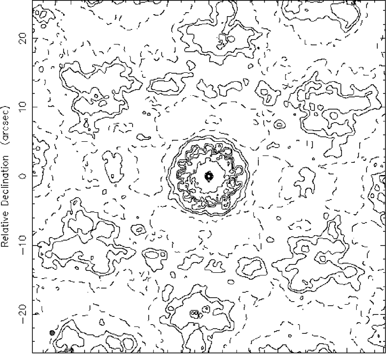
“Multiresolution Cleaning” (Wakker & Schwarz, 1991) is an extension to CLEAN that aims to improve upon CLEAN’s handling of extended emission (e.g. Figure 6) by using not just one CLEAN beam, but a set of CLEAN beams of different scales. In practice two variations, multi-scale CLEAN (Cornwell & Holdaway, 2006) and adaptive scale pixel (ASP) decomposition (Bhatnagar & Cornwell, 2004) work better and differ in how they use and set the variously scaled beams. For structures larger than the standard CLEAN beam their behavior should fall somewhere between smear fitting and standard CLEAN if natural weighting is used, with somewhat reduced flexibility because of the finite number of choices. Practitioners can however in principle preload the algorithms with elongated gaussians if needed, and ASP dynamically updates its set of scales. Structures smaller than the standard CLEAN beam can be resolved if sharp enough beams are used but such resolution (as in the bottom of Figure 7) is not reliable since CLEAN and its derivatives do not have a signal to noise based mechanism for testing resolution. Much more effort has been put into their ability to recover structures the size of the standard CLEAN beam and larger.

Figure 7: Deconvolutions of a section of the Canadian Galactic Plane Survey (Taylor et al., 2003) including many AGN and the less sharp galactic HII region Sharpless 155. Top: smear fitted. Middle: multiscale CLEANed and restored with a gaussian fit to the uniformly weighted dirty beam. Bottom: multiscale CLEANed without convolution by a CLEAN beam. Convolution by the standard CLEAN beam obscures too much detail, but doing without it leaves the compact sources as $\delta$ functions embedded in the next larger gaussian used by multiscale CLEAN. A square root function has been used for the grayscale intensity mapping.

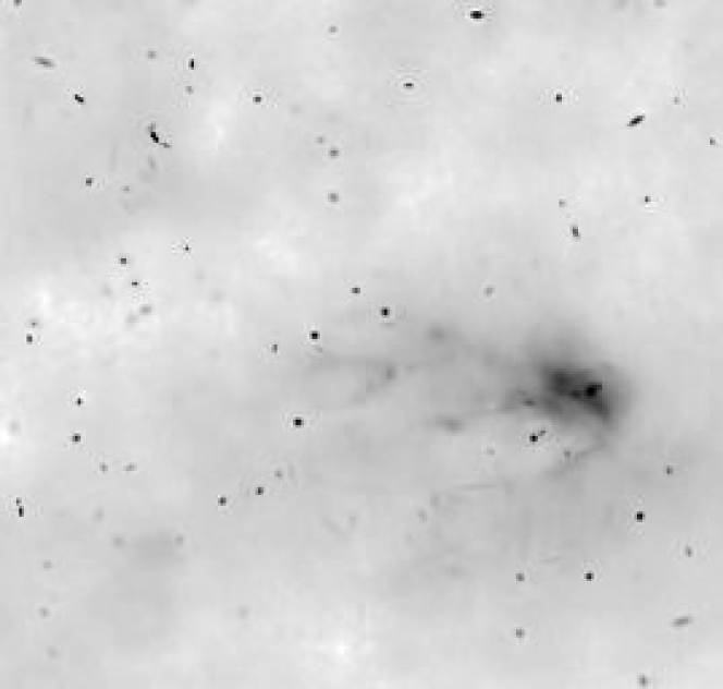
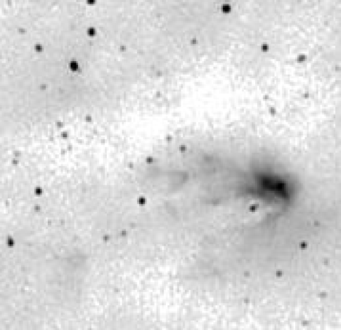
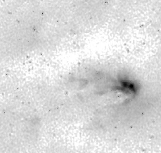
3.1.5 Self-calibration

Smearing assumes that the measurement errors are normally distributed noise, but the quality of many data sets is limited by calibration errors, which must be corrected by selfcalibration Cornwell & Wilkinson (1981). Selfcalibration assumes (but is constrained in its action when the number of receivers is greater than four) that the model includes most of the source and that the residuals are mostly due to calibration errors. Amplitude selfcalibration in particular can be dangerous with classical CLEAN since traditional CLEAN picks the brightest peaks first, and leaves behind any real structure that is fainter than the calibration error induced artifacts around bright peaks. This results in a tendency of amplitude selfcalibration to distort the gains of central antennas if applied carelessly. Smear fitting and multiresolution CLEAN are both able to fit broad features at an early stage, making it possible in most cases to apply selfcalibration before calibration errors threaten to contaminate their models and prevent convergence on the correct solution.

3.1.6 Comparisons using known brightness distributions

Figure 8: The reference image “observed” by the simulations, based on a smear fitted model of a 4.7 GHz VLA A and B array observation of the northern two–thirds of J012435-040105, with some faint (restored) CLEAN components, both positive and negative, included. The contours start at 20 $\mu$Jy/arcsec² and each is separated by a factor of 2 from its neighbor(s).

Figure 9: Image, using the true model, of a simulated 4.7 GHz VLA B array observation of Figure 8 placed at a declination of $+30^{\circ}$. The contours start at 50 $\mu$Jy/arcsec² and each is separated by a factor of 2 from its neighbor(s). The solid gray ellipse in the lower left corner shows the FWHM extent of the dirty beam.

Figure 10: A smear fitted image made using the same data, contours, and beam as Figure 9.

Figure 11: CLEAN deconvolutions of the same simulated observation used in Figure 9. Top: naturally weighted image with the same contours as Figure 9. Bottom: uniformly weighted image with contours starting at 0.2 mJy/arcsec², each separated from its neighbor(s) by a factor of 2. The solid gray ellipses in the lower left corners shows the FWHM extent of the dirty beam.

Figure 12: Deconvolutions made from a simulated 8 hour VLA B array observation of Figure 8 placed at a declination of $+30^{\circ}$. Top: smear fitted image with contours starting at 10 $\mu$Jy/arcsec². Bottom: uniformly weighted CLEAN image with contours starting at 50 $\mu$Jy/arcsec². Each contour is separated by a factor of 2 from its neighbor(s), and the solid gray ellipses in the lower left corner shows the FWHM extent of the dirty beams.

Figure 13: Deconvolutions made from a simulated VLA A array snapshot of Figure 8 placed at a declination of $+30^{\circ}$. Top: smear fitted image with contours starting at 0.5 mJy/arcsec². Bottom: naturally weighted CLEAN image with contours starting at 0.8 mJy/arcsec². Each contour is separated by a factor of 2 from its neighbor(s), and the solid gray ellipses in the lower left corner shows the FWHM extent of the dirty beams.

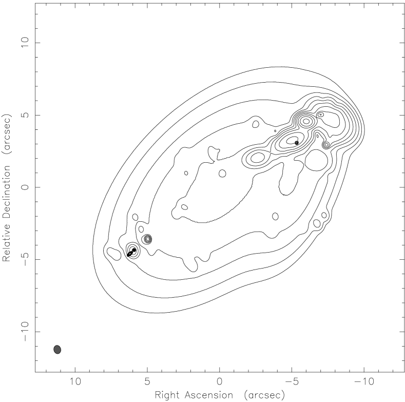
Figures 8 to 13 present the responses of CLEAN and smear fitting to a fairly complex source under a variety of conditions. In order that the true image could be known, and to dispense with the effects of calibration errors, Miriad’s (Sault et al., 1995) uvgen command was used to simulate VLA observations (with noise) of a given model. To make the input model representative of a real observation, it includes the northwest jet and core of a smear fitted model made with the combination of several VLA A and B array snapshots of J012435–040105 (Reid et al., 1999). A smear fitted model was used because it was the best source of both very sharp and broad realistic structure available. The morphology of this source is also very challenging since it contains a sharp feature of moderate flux density embedded in a broader stream, and the jet bends over on itself into a crook. The overall envelope of the jet was enhanced by the addition of a broad elliptical gaussian. To prevent the model from being completely composed of smear fitting’s stock in trade, several dozen CLEAN components (restored with the A array beam), both positive and negative, were randomly scattered around the jet. Note that the CLEAN component positions are completely random and not centered on pixels.

In the simulated B array observations (Figures 9 to 12) the challenge was to resolve the three sharp peaks near the core and as much of the jet morphology as possible. Smear fitting did much better, even when uniform weighting was used for CLEAN. Neither of the algorithms managed to resolve the two peaks closest to the core. The smear fitted image of the extended observation (Figure 12) did very well otherwise, while the CLEAN image was only able to improve its sensitivity, not its resolution. In theory the resolution of a smear fitted image can improve without bound as data of the same average baseline length is added, but in practice the improvement would eventually be limited by calibration errors.

With the simulated VLA A array observation, Figure 13, of Figure 8, smear fitting leaves the diffuse emission mainly to the imagination of the viewer, although it could be argued that there is a statistically significant enhancement of the density of small peaks in the region of the diffuse emission. Away from the emission region the residuals are satisfyingly noise-like, but ironically the broad negative artifacts to the north and south of the jet in the CLEAN image announce to the connoisseur the possible existence of badly imaged diffuse emission.

3.2 Maximum Entropy

Smear fitting and CLEAN look for structure in the image plane and then impose smoothness based on $uv$ plane considerations, but maximum entropy deconvolution (Cornwell et al. 1999, Cornwell & Evans 1985), or ME, takes a different approach by starting with a (usually) smooth default image (the prior) and trying to maintain smoothness in the image plane as structure is imposed by the visibilities. Otherwise it has the same goal as smear fitting: to produce the smoothest image possible within the constraints of the data. In ME deconvolution each pixel is considered to be a variable, but smear fitting can be considered as a type of ME where the variables are a set of model parameters. This is not to say that smear fitting with an elliptical gaussian for each pixel would be equivalent to traditional ME. First, each gaussian has 6 degrees of freedom, while a pixel only has one. More importantly, in traditional ME it is the distribution of pixel intensities that is compared to the measurements, while smear fitting calculates $\chi^{2}$ for the set of model parameters.

The choice of definition for the entropy function, ${\cal H}$, to be maximized, is controversial (Narayan & Nityananda, 1984) but the most popular one is

$${\cal H}=-\sum_{k}I_{k}\ln\frac{I_{k}}{M_{k}e}$$ (11)

where $I_{k}$ and $M_{k}$ respectively are the intensities of the $k$th image and prior pixels. Equation 11 can only be used for positive images, but other functions which are between linear and quadratic, like

$${\cal H}=-\sum_{k}\ln\left(\cosh\frac{I_{k}-M_{k}}{\sigma}\right)$$ (12)

where here $\sigma$ is the noise level in the image, also provide smoothing, and have been used for polarization images. All of these functions, however, only consider the sum of functions of individual pixels. This is hazardous since the data, being in the $uv$ plane, are more directly connected with the relationships between neighboring pixels than the values of individual pixels. In particular, if the source has a sharp peak on top of a diffuse background, the background dilutes the smoothing power that $\cal{H}$ would get from its steepness at very low intensities, and the peak is left partly dirty (Figure 14).

Figure 14: Ringing in a maximum entropy image, made using the AIPS task VTESS, of the simulated data used in Figure 6. The contours start at 40 mJy/arcsec² and are each separated by a factor of 2.

Another criticism of traditional ME is that the default prior image, a flat distribution, is actually a very unlikely state for an interferometric image (unless nothing has been observed!). ME is thus biased toward putting flux in pixels that should not have any, as in Figure 4. Smear fitting, like CLEAN, is more accepting of negative pixels, although both often use positivity as a constraint when constructing their models.

Smear fitting and ME both produce final results that are biased away from the best fit to the measurements, but they have their justifications. ME has two, the first being the importance of not claiming anything that is not absolutely necessary, or in other words maximizing the entropy. The second justification is simply that ME produces better images with the bias than without it (simulatable by making the uncertainties approach zero). Smear fitting adds the goal of trying to estimate the probability distribution of where the measured light may have originated from. Seen this way, it is not biased at all, if the uncertainty determination is correct.

Figure 15: Comparison of maximum entropy and CLEAN to smear fitting, for a low elevation observation of J125720–333450 (Reid et al., 1999). The contours start at $\pm$ 0.032 mJy per square arcsecond, and increase by a factor of two between successive contours. Each map used the same dataset, self–calibrated using smear fitting. The bottom left graph plots the intensity of each pixel in the smear fitted (vertical axis) image against that of the same pixel in the maximum entropy (horizontal axis) image.

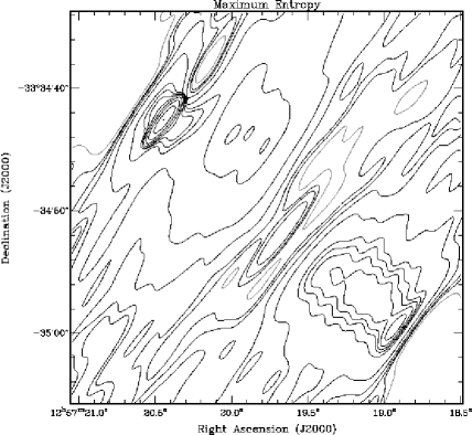
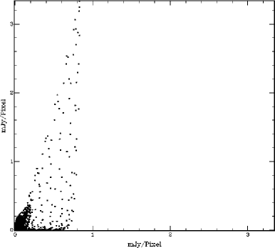
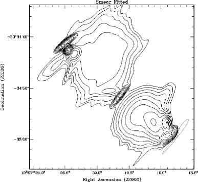
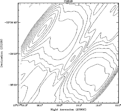
Figure 15 illustrates the similarity of maximum entropy to smear fitting, although it may not look like it at first glance since the largest and most distracting contours are the faintest and least reliable. It was not feasible to deconvolve down to the noise, or even the rms level of the smear fitting residuals, with maximum entropy, with any of the large sample of VLA snapshots of jets in Reid et al. (1999). That is partly due to the hot spots that all jets have. Normally they would be CLEANed away before applying maximum entropy, but as the CLEAN image shows, convolving the three brightest points with the CLEAN beam would have hidden much of the structure. Also, it could be that pixel–by–pixel flexibility of maximum entropy leaves it more vulnerable to the sampling sparseness of the snapshot survey, which could effectively act as an additional apparent noise source.

Nevertheless, when the lowest contours are ignored, the ME and smear fitted maps are quite similar, and both show an effective beam for bright emission that is much smaller and less elongated than CLEAN’s. The lower left corner of Figure 15 quantitatively compares them by graphing the intensity of each smear fitted pixel against the intensity of the corresponding pixel in the ME map. If the images were identical, the locus of points would be a straight line with slope 1. Obviously the range of maximum entropy pixel values is only about a quarter of that in the smear fitted image. This cannot be fully accounted for by the maximum entropy image being “dirtier”, since that mainly affects the faintest pixels. This may be due to maximum entropy treating entropy as a global property of the image, while smear fitting treats entropy (smearing, roughly) as a local property of each component. Smear fitting thus prevented from wrongly transferring flux between separated features in order to lower the overall sharpness of the image. Indeed, the sharpest components tend to have the most signal and are smeared least.

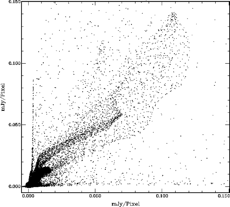
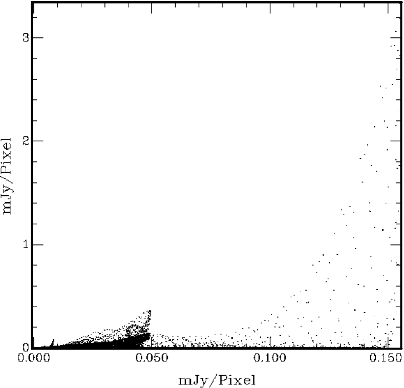
Smear fitting and ME match more closely at medium intensities, as shown by Figure 16. CLEAN (Figure 17), however, does not approach a one-for-one match with smear fitting except at very low intensities, where ME also has a short dense locus of points with overall slope 1 (the inner 15 $\mu$Jy of Figure 16). Those pixels are in the northwest lobe, where because it is broad and flat the pixel values are not strongly affected by convolution with any beam the size of the CLEAN beam or smaller.

Figure 16: The fainter pixel intensities of the smear fitted (vertical axis) and ME (horizontal axis) images of Figure 15.

Figure 17: The pixel intensities of the smear fitted (vertical axis) and CLEAN (horizontal axis) images of Figure 15. Note that the dynamic range of the CLEAN axis is much smaller than that of the smear fitted axis.

3.3 Pixel Based Models

All existing deconvolution methods produce a rectangular array of pixel values as their final image, but there is no fundamental reason why their internal representation of the source should also be a rectangular array of pixel values. Although the desired output, an image capable of being displayed on common computer hardware, is a set of pixels, the input measurements are an irregular array of visibilities, and operations which need to consider measurement uncertainty tend to be more practical when performed in the same basis as the measurements. One of the motivations of smear fitting was to bring imaging conceptually closer to the measurements, and as a result the models used in smear fitting have no explicit dependence on pixel size or shape.

More prosaically, the locations of the component centers in smear fitting are not quantized to land on pixel centers. In many algorithms, including ME and non-negative least squares (NNLS, Briggs (1995)) deconvolution, the model is a set of pixels, and in commonly available implementations of CLEAN the model components are only placed on pixel centers (although in principle they do not need to be). Pixels poorly represent features that are centered on pixel edges, which can degrade the usefulness of pixel based models for selfcalibration. Perley (1999) has also shown that a sharp feature centered on a pixel edge cannot be represented by pixel centered CLEAN components without violating the positivity constraint.

The Pixon deconvolution method (Puetter & Yahil, 1999) shares with smear fitting the concept that the model (a preliminary image in Pixon’s case) should be smoothed as much as possible within the constraints of the data, and that the amount of smoothing should be determined locally, not from a global prior as with ME. Instead of smear fitting’s procedure of fitting a model to the measurements by minimizing $\chi^{2}$ and then smoothing that model, the Pixon method convolves each pixel in a model image with the largest acceptable kernel in a list of typically a dozen gaussians. The Pixon technique thus uses a pair of variables (flux and kernel size) for each pixel, while smear fitting eschews pixels and attempts to model the source with the minimum number of parameters, typically several dozen, required by the visibilities.

$\chi^{2}$ minimization adjusts the model to maximize the probability of the data given the model, so smear fitting could be broadly classified as a smoothed maximum a posteriori probability (MAP) algorithm, while the Pixon method results in a similarly smoothed NNLS image. As a NNLS variant, the Pixon method cannot represent sources with both positive and negative emission. Bhatnagar & Cornwell (2004) also note that the Pixon method is not suited to interferometry, since the algorithm relies on a compact point source response function (i.e. a dirty beam which is zero outside a finite region), and noise that is independent and additive in the image plane.

3.4 Processing speed

Smear fitting tends to be somewhat slower than CLEAN, but not prohibitively so, and most observations can be smear fitted using standard hardware in a reasonable length of time. Quantifying the speed of smear fitting relative to CLEAN or Maximum Entropy can be done for a few examples, but extrapolating from those examples to all observations is nearly impossible, because the speed of smear fitting depends most strongly on the observation’s “complexity”, which is itself difficult to measure. The complexity increases with the number of components, but also depends on how much coupling there is between the components and how well the observation can be modeled with the given set of basis functions. To give some scale to “not prohibitively”, using a 1.6 GHz Athlon CPU, CLEAN took one minute to produce the naturally weighted image of Figure 11 while smear fitting took twenty minutes to deconvolve the same simulated VLA snapshot (Figure 10). Neither algorithm was hampered by a lack of RAM or the need to self-calibrate.

To some extent the speed of other deconvolution methods is also affected by source complexity, but to first order the processing time required by ME is set by the number of pixels, while CLEAN’s depends on the number of pixels with significant brightness, being faster than Maximum Entropy for typical VLA images with up to $10^{6}$ active pixels (Cornwell et al., 1999).

Fitting a gaussian is more time consuming than placing a CLEAN component, but one gaussian, or even better a specially selected function, in smear fitting corresponds to many CLEAN components. Typically CLEAN images have thousands of components, while smear fitting only uses a few dozen, and the flux of each CLEAN component is typically built up with 5 to 100 steps (a gain of 0.2 to 0.01). Smear fitting can be the fastest method for simple but extended sources and/or a small number ($\lesssim 50000$) of visibilities. Note however, that although the runtime of a single iteration of $\chi^{2}$ minimization is proportional to the number of visibilities, improving the dirty beam with more $uv$ samples can make component specification more efficient and reduce the number of $\chi^{2}$ minimization iterations needed.

The number of visibilities can be effectively lowered without drastically degrading the dirty beam by binning them. Normally binning the visibilities should be avoided since it can create problems (Briggs, 1995) and is not required when smear fitting. Fortunately large data sets that are enough to make smear fitting annoyingly slow also tend to have dense $uv$ coverage, eliminating many of the ambiguities that can impede model construction, and making them good candidates for binning. More importantly, smear fitting does not use uniform weighting, which is responsible for most of the imaging problems with binning.

4 Discussion

Deconvolution by fitting simple models to the visibilities using $\chi^{2}$ minimization is by no means new. In fact it predates CLEAN (Högbom, 2003) but garnered a reputation of being difficult and unreliable. The most serious problem with traditional model fitting, at least for imaging, is that components corresponding to unresolved features can, and probably will, collapse into Dirac $\delta$ distributions or knife-edges. Smearing explicitly does away with that problem by convolving each component with an elliptical gaussian set by the uncertainty of the component’s shape and location. The other commonly heard complaint traditional model fitting is that a model must be supplied before its parameters can be fit to the data, and in the typical case of incomplete data it is impossible to be sure that the model both has the right variables and started in the correct (i.e. global) local minimum of $\chi^{2}$. In other words, different astronomers can derive different results from the same data because they started with different initial models based on their subjective choices. Of course, that situation is not unique to imaging, but objectivity is still worth striving for. Smear fitting removes some of the subjectivity in the final image by smearing the statistically insignificant details, but more pertinently its implementation as a patch to difmap promotes automatic model construction. Practitioners of smear fitting should only rarely need to intervene in the model construction process, for example by choosing to model a feature with an alternative functional form to an elliptical gaussian, and in such cases should be able to support their choice based on an improvement in $\chi^{2}$ or positivity, or data from other wavebands.

Smear fitting may appear to smear more than CLEAN for low surface brightness objects, but it must be remembered that whatever is smeared out of the model is returned to the dirty residuals. Usually the CLEAN beam size is matched to the dirty beam, so smear fitting does not produce worse resolution than CLEAN. Unfortunately the image is not the definitive place to determine whether sub–beam features are extended. To properly answer that question the reverse of smear fitting should be done; collapse the component(s) down to a single Dirac $\delta$ distribution and check whether $\chi^{2}$ is raised above the minimum by at least twice the number of parameters specifying the original shape. The smerf patch does not provide a command to automatically perform this check, but it is easy enough to do on a case-by-case basis. These properties of variable resolution also apply to ME if it is not convolved with a CLEAN beam at the end(Cornwell et al., 1999), although the test for resolution, by minimizing the entropy, would in general not be as useful since ME works on an entire image at a time instead of specific features.

4.1 Sensitivity and weighting

Although smear fitting cannot deconvolve low surface brightness features any better than the other methods, its use is beneficial to being able to detect them. Smear fitting uses the most sensitive weighting scheme, natural weighting, while the other methods often downweight the inner visibilities to produce a sharper and more gaussian dirty beam. Robust weighting (Briggs, 1995) is a considerable improvement over uniform weighting, but natural weighting still gives the greatest surface brightness sensitivity. All deconvolution methods can use natural weighting, but it produces a large beam, and no fixed resolution method can distinguish faint emission from bright peaks when they are within a beamwidth of each other.

Uniform or superuniform weighting hurts the sensitivity to sharp as well as diffuse objects by effectively ignoring central visibilities even though they measure the flux of sharp features just as well as the long baseline visibilities (ignoring possible differences in antenna sensitivities). Smear fitting uses all visibilities for detection of flux, so that the position of a visibility simply affects its leverage on the resolution.

More subtly, smear fitting avoids the most common errors in fitting the bright features that typically limit the dynamic range of images deconvolved using other methods. The first two of these errors are due to premature pixelization in order to use the Fast Fourier Transform (FFT). The FFT requires the visibilities to be placed in rectangular bins, and outputs the result in rectangular pixels. This introduces firstly a quantization error to the positions of the visibilities. Secondly, if anything but natural weighting is used, it can have disastrous effects if a visibility is placed in a bin by itself when most visibilities share their bin with several others. Uniform weighting would give the lone visibility as much weight as a large batch of visibilities in a nearby bin, thereby amplifying the error of the lone visibility (Briggs, 1995). Smear fitting avoids binning by using analytical Fourier transforms for its model components. The final image is displayed using pixels, but there is no error generated in the Fourier transformation of the model. The residuals still use the FFT, but typically in the final image their dynamic range is so low that the introduced error is negligable.

4.2 Beam elongation

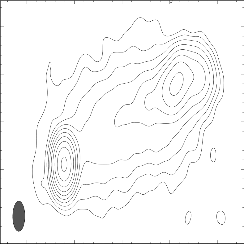
A notable advantage of smear fitting is that it is less affected by the source elevation angle than CLEAN (Figure 18). The axial ratio of an east–west interferometer’s dirty beam is the absolute sine of the source’s declination, meaning that the major axis approaches infinity for objects near the celestial equator. Similarly, an array with both east–west and north–south baselines has foreshortened $uv$ coverage for low elevation sources, so many observations have strongly elliptical dirty beams that distort the appearance of their features. CLEAN can mask that distortion by using a round restoring beam with the same radius as the semimajor axis of the dirty beam, but at the cost of losing resolution along the minor axis. Smear fitting copes better, since the density of baselines goes up when they are compressed along one axis. Thus a component that is resolved along that axis will have more visibilities brought in to where it needs them, so its signal to noise ratio will improve and it will not be smeared as much (see Table 1). Less resolved features benefit less, since for them the effect on $\chi^{2}$ (i.e. resistance to smearing) of a visibility is proportional to the fourth power of the baseline length, so the outer baselines dominate (Appendix A). If the unresolved features are bright their major axes will be strongly affected by the baseline foreshortening, but if they are faint enough for the Fourier transform of their smearing beams to be enclosed by the envelope of where there are visibilities, they also experience the rounding effect.

xD..4 yD..5

	Feature		Smearing beam
$\delta$ (°)	FWHM (″)	$I_{\textit{\scriptsize peak}}/I_{\textit{\scriptsize rms}}$	FWHM (″)	Axial ratio
		423.4	0.067	0.480
	0.20	43.23	0.235	0.523
		39.00	0.416	0.970
	2.00	3.90	1.57	0.949
-30	CLEAN beam		0.964	0.404
		384.2	0.039	0.829
	0.20	38.36	0.131	0.850
		46.16	0.431	0.903
	2.00	4.08	1.21	0.961
0	CLEAN beam		0.509	0.766
		373.5	0.036	0.962
	0.20	37.09	0.126	0.975
		40.88	0.454	0.863
	2.00	4.13	1.367	0.921
30	CLEAN beam		0.423	0.922

Table 1: Smearing beam dependence on source declination for simulated VLA A Array snapshots on the meridian. Note that $I_{\textit{\scriptsize peak}}$ is the surface brightness in the dirty map.

Figure 18: Deconvolved images of a simulated VLA B array snapshot of Figure 8 at a declination of $-30^{\circ}$. Top: CLEAN. Bottom: smear fitted. The solid gray ellipses are the half maximum extent of the CLEAN beam (same in both) and the contours start at 25 $\mu$Jy/arcsec², with each separated by a factor of 2 in brightness.

4.3 Customized component types

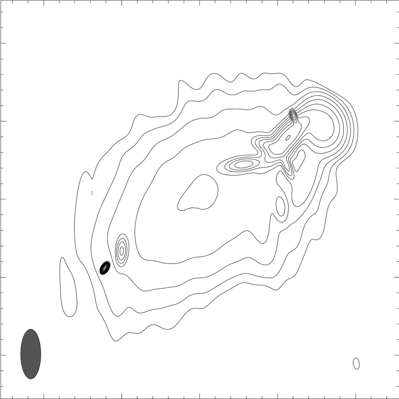
Elliptical gaussians are convenient basis functions for modelling most sources, but some objects, especially ones that have steep edges and known physical forms, are better fit if different functions are introduced. Figure 2 shows four deconvolutions of a VLA snapshot of a planetary nebula, Vy2-2 (Christianto & Seaquist, 1998). Vy2-2 is young and well described at 15 GHz by an optically thin shell. The shell was only moderately resolved by CLEAN, and smear fitting with elliptical gaussians either broke the symmetry of the source or produced a unphysically negative center for the shell. The ring could be better approximated by using more gaussians, but splitting the the flux into smaller portions would enlarge the smearing beam for each component. Ideally smear fitting should use as few parameters as necessary, and the right framework (or model type) for those parameters. The difmap and the smerf patch do not explicitly have optically thin shells as a component type (although optically thick ones are available as flat disks), but one can be easily constructed by placing a negative optically thin ellipsoid (OTE) inside a positive one. Since the pair correspond to a single feature, and especially since it is the difference of their flux densities, not their individual flux densities, that is physically meaningful, smearing gaussians were calculated for them simultaneously instead of serially. The result was a much better fit, and the possibility of measuring the geometrical thickness of the shell.

4.4 Future possibilities

Model fitting by minimizing $\chi^{2}$ is extremely flexible, and could be extended beyond providing a choice of component types. One avenue for future work would be to combine data from multiple polarizations and/or frequencies while applying constraints (for example $Q^{2}+U^{2}+V^{2}\leq I^{2}$ and/or a spectral index) on how the components should appear in each subset of the data. Although such dynamic constraints have not yet been used with smear fitting, it is already possible to construct a model using one set of data and use it as the initial model with related data sets. For example, the positions of a set of isolated unresolved objects are the same for all polarizations and frequencies, so a model of the set can be produced and smeared in Stokes I, and then the Q and U models can be obtained by simply refitting the fluxes without needing to change the smears.

5 Conclusion

Smear fitting is an image deconvolution method that fits a near maximally simple model to interferometer visibilities and then broadens the model to account for the uncertainty of those visibilities. The model construction method avoids several problems that can limit the quality of CLEAN and maximum entropy deconvolutions, and smearing generally yields sharper and fairer images than CLEAN.

As mentioned above, smear fitting has been implemented as a modification (patch) to difmap, a well known program for imaging and selfcalibrating data from radio interferometers. The patch, known as smerf, is freely available under the GNU license (Stallman, 1991) at http:$/\!$/www.drao-ofr.hia-iha.nrc-cnrc.gc.ca/$\!\sim$rreid/smerf/, and includes a manual on its use.

Appendix A Baseline leverage

Consider a feature modeled by a circular gaussian with flux $f$ and FWHM $a$. We can without loss of generality place the phase tracking center at its location, so that the model visibilities $V_{m,i}$ are $f\exp\left(-0.36a^{2}u_{i}^{2}\right)$, where $u_{i}$ is the length of baseline $i$. Writing the differences between the measured and model visibilities as ${\sf\epsilon}_{i}$,

$$\chi^{2}_{\textit{\scriptsize unsmeared}}=\sum_{i}\left|{\sf\epsilon}_{i}/\sigma_{i}\right|^{2}$$ (13)

Smearing the component with a round gaussian with FWHM $a_{s}$ multiplies the model visibilities by $\beta(a_{s}^{2}u_{i}^{2})\equiv\exp\left(-0.36a_{s}^{2}u_{i}^{2}\right)$. (This discussion can easily be extended to an elliptical smearing beams, but it is not warranted here.) The expected rise in $\chi^{2}$ due to smearing is

$$\Delta\mbox{$\chi^{2}$} \equiv \chi^{2}_{\textit{\scriptsize smeared}}-\chi^{2}_{\textit{\scriptsize unsmeared}}$$ (14)

$$= \sum_{i}\frac{1}{\sigma_{i}^{2}}(1-\beta)V_{m,i}\left[(1-\beta)V_{m,i}+2{\sf\epsilon}_{i}\right]$$ (15)

The leading term in a Maclaurin expansion of $1-\beta$ is $0.36a_{s}^{2}u_{i}^{2}$, so if the component is sharp (nearly flat in the $uv$ plane), the ${\sf\epsilon}_{i}$ are small, and there is little smearing, the effect of a visibility on $\Delta\mbox{$\chi^{2}$}$ is proportional to the fourth power of its baseline length. If the component is resolved $V_{m,i}$ attenuates the importance of the outer baselines. Their special status can also be removed by a large smearing beam, since $1-\beta$ saturates at 1.

Note that this leverage is simply the relative importance of the visibility. Since $\beta$ is a function of the product of $a_{s}$ and $u_{i}$, $a_{s}$ is inversely proportional to an average baseline length, as one would expect, but the average is weighted towards the outer regions of where there is significant measured amplitude in the $uv$ plane.

References

- Bhatnagar & Cornwell (2004) Bhatnagar S., Cornwell T. J., 2004, Astronomy & Astrophysics, 426, 747
- Born & Wolf (1999) Born M., Wolf E., 1999, Principles of Optics, 7 edn. Cambridge University Press, pp 370–372
- Briggs (1995) Briggs D. S., 1995, PhD thesis, New Mexico Institute of Mining and Technology
- Christianto & Seaquist (1998) Christianto H., Seaquist E. R., 1998, AJ, 115, 2466
- Cornwell & Holdaway (2006) Cornwell T., Holdaway M., 2006, submitted to Astronomy & Astrophysics
- Cornwell et al. (1999) Cornwell T. J., Braun R., Briggs D. S., 1999, in Taylor G. B., Carilli C. L., Perley R. A., eds, Synthesis Imaging in Radio Astronomy II Vol. 180 of ASP Conference Series, Deconvolution. pp 151–170
- Cornwell & Evans (1985) Cornwell T. J., Evans K. F., 1985, Astronomy & Astrophysics, 143, 77
- Cornwell & Wilkinson (1981) Cornwell T. J., Wilkinson P. N., 1981, MNRAS, 196, 1067
- Gull & Skilling (1983) Gull S. F., Skilling J., 1983, in Indirect Imaging. Measurement and Processing for Indirect Imaging. Proceedings of an International Symposium held in Sydney, Australia, August 30-September 2, 1983. Editor, J.A. Roberts; Publisher, Cambridge University Press, Cambridge, England, New York, NY, 1984. LC # QB51.3.E43 I53 1984. ISBN # 0-521-26282-8. P.267, 1983 The Maximum Entropy Method. pp 267–+
- Högbom (1974) Högbom J. A., 1974, Astronomy & Astrophysics Supplement, 15, 417
- Högbom (2003) Högbom J. A., 2003, in ASP Conf. Ser. 300: Radio Astronomy at the Fringe Early Work in Imaging. pp 17–20
- Narayan & Nityananda (1984) Narayan R., Nityananda R., 1984, in Roberts J. A., ed., Indirect Imaging Maximum entropy – flexibility versus fundamentalism. Cambridge University Press, Cambridge, England, pp 281–290
- Pearson (1999) Pearson T. J., 1999, in Taylor G. B., Carilli C. L., Perley R. A., eds, Synthesis Imaging in Radio Astronomy II Vol. 180 of ASP Conference Series, Non–imaging data analysis. pp 335–354
- Perley (1999) Perley R. A., 1999, in Taylor G. B., Carilli C. L., Perley R. A., eds, Synthesis Imaging in Radio Astronomy II Vol. 180 of ASP Conference Series, High dynamic range imaging. pp 275–299
- Puetter & Yahil (1999) Puetter R. C., Yahil A., 1999, in ASP Conf. Ser. 172: Astronomical Data Analysis Software and Systems VIII The Pixon Method of Image Reconstruction. pp 307–+
- Reid (2003) Reid R. I., 2003, PhD thesis, University of Toronto
- Reid et al. (1999) Reid R. I., Kronberg P. P., Perley R. A., 1999, ApJS, 124, 285
- Sault et al. (1995) Sault R. J., Teuben P. J., Wright M. C. H., 1995, in ASP Conf. Ser. 77: Astronomical Data Analysis Software and Systems IV A Retrospective View of MIRIAD. pp 433–+
- Shepherd (1997) Shepherd M. C., 1997, in A.S.P. Conf. Ser. 125: Astronomical Data Analysis Software and Systems VI Vol. 6, Difmap: an Interactive Program for Synthesis Imaging. pp 77+
- Stallman (1991) Stallman R. M., , 1991, GNU General Public License
- Taylor et al. (2003) Taylor A. R., Gibson S. J., Peracaula M., Martin P. G., Landecker T. L., Brunt C. M., Dewdney P. E., Dougherty S. M., Gray A. D., Higgs L. A., Kerton C. R., Knee L. B. G., Kothes R., Purton C. R., Uyanıker B., Wallace B. J., Willis A. G., Durand D., 2003, AJ, 125, 1350
- Wakker & Schwarz (1991) Wakker B. P., Schwarz U. J., 1991, in ASP Conf. Ser. 19: IAU Colloq. 131: Radio Interferometry. Theory, Techniques, and Applications The multi-resolution clean. pp 268–271