Sérsic Properties of Disc Galaxy Mergers

Abstract

Sérsic parameters characterising the density profiles of remnants formed in collision-less disc galaxy mergers are obtained; no bulge is included in our simulations. For the luminous component we find that the Sérsic index is $n\!\in\!(1.5,5.3)$ with $\langle n\rangle\approx 3\pm 1$ and an effective radius of $R_{\rm e}\!\in\!(1.6,12.9)\,$kpc with $\langle R_{\rm e}\rangle\approx 5\pm 3\,$kpc. The mean values of these quantities increases as the radial interval of fitting is reduced. A strong correlation of $n$ with the central projected density $I_{0}$ is found ($n\propto I_{0}^{-0.14}$) which is consistent with observations. No positive linear correlation between the size ($R_{\rm e}$) and structure ($n$) of our remnants is found; we do not advocate the existence of this. The photometric plane (PHP) of the luminous component ($n\propto R_{\rm e}^{0.05}I_{0}^{0.15}$) agrees well, within the uncertainties and the assumption of a constant mass-to-light ratio, with those observationally determined for ellipticals in the $B$-band ($n\propto R_{\rm e}^{0.09}I_{0}^{0.15}$) and for $K$-band remnants ($n\propto R_{\rm e}^{0.11}I_{0}^{0.14}$). We found that the surface defined by Sérsic parameters $\{n,R_{\rm e},\mu_{0}\}$ in log-space is not a true plane, but a pseudo-plane with a small curvature at low values of $n$ owed to intrinsic properties of the Sérsic model. The dark haloes of the remnants have a 3-dimensional Sérsic index of $\langle n\rangle\approx 4\pm 0.5$ that are smaller than the ones obtained for dark haloes in $\Lambda$CDM cosmologies $n\approx 6\pm 1$. A tight dark Sérsic “plane” (DSP) is also defined by the parameters of the remnants haloes with $n\propto r_{\rm e}^{0.07}\rho_{0}^{0.10}$. We conclude that collision-less merger remnants of pure disc galaxies have Sérsic properties and correlations consistent with those of observed in early-type galaxies and local remnants. It seems that a “primordial” bulge in spirals is not a necessary condition to form bona fide ellipticals on grounds of the Sérsic properties of remnants.

1 Introduction

Hierarchical galaxy formation theory (e.g. Cole et al. 2000, De Lucia et al. 2005, Bower et al. 2005) considers that early-type galaxies have an accretion/merger origin, as was originally suggested by Toomre (1977). Observational (e.g. Schweizer 1998, Struck 2005, Rothberg & Joseph 2006, Kaviraj et al. 2006) and theoretical (e.g. Naab & Burkert 2003, Meza et al. 2005, Naab et al. 2005) evidence supports this picture although several topics remain unsolved (e.g. Peebles 2002, Tantalo & Chiosi 2004).

Early-type galaxies show several correlations among their colours, luminosities, velocity dispersions, effective radii and surface brightness (e.g. Baum 1990, Faber & Jackson 1976, Kormendy 1977, Djorgovski & Davis 1987, Dressler et al. 1987, Bernardi et al. 2003). These correlations provide constraints to any theory of formation and evolution of these galaxies. Furthermore, their properties are linked with the distribution of luminous and dark matter, that would be important when comparing with models of formation of elliptical galaxies.

Observational studies [e.g. Caon, Capaccioli & D’Onofrio 1993 (CCD93), Graham & Colles 1997, Binggeli & Jerjen 1998, D’Onofrio 2001 (D01), Trujillo et al. 2004] have found that the surface brightness density profiles of early-type galaxies are better described by a Sérsic (1968) $R^{1/n}$–profile than the classical de Vaucouleurs (1948) $R^{1/4}$–profile. The index $n$ is directly related with the curvature and “concentration” of the light profile (Trujillo, Graham & Caon 2001).

Several observational relationships have been found between the index $n$ and, for example, the total luminosity ($L$), effective radius ($R_{\rm e}$) and central velocity dispersion (e.g. CCD93, Prugniel & Simien 1997, Graham & Guzmán 2003). Also, it has been found a linear relation among $\log n$, $\log R_{\rm e}$ and $\mu_{0}$ (central brightness) termed the Photometric Plane (PHP) for early-type galaxies [e.g. Khosroshahi et al. 2000 (K00), Graham 2002], analogous to the Fundamental Plane (Djorgovski & Davis 1987, Dressler et al. 1987). Recently, Rothberg & Joseph (2004, RJ04) have found that nearby merger remnants have a peak in the $n$-distribution at $n\approx 2$ with most values in the range of $1<n<6$, and in some cases it is found that $n>8$.

On other hand, theoretical studies of Sérsic properties of merger remnants have appeared recently. For example, Gónzalez-García & Balcells (2005, GGB) and Naab & Trujillo (2005, NT) find in collision-less simulations that bulge-less progenitors lead to ranges of $n\!\in\!(2.4,3.2)$ and $(1.2,3.1)$, respectively; when a single Sérsic function is used to fit the entire remnant. For progenitors with a bulge component they obtain about the same range of Sérsic index, $n\!\in\!(3,8)$. Since “bona fide” ellipticals have values $n\mathrel{\hbox to0.0pt{\lower 3.0pt\hbox{$\mathchar 536\relax$}\hss}\raise 2.0pt\hbox{$\mathchar 318\relax$}}4$, they reach the conclusion that collision-less merger remnants of pure disc galaxies do not lead to concentrations, indicated by $n$, similar to those found in intermediate or giant elliptical galaxies (e.g. Graham et al. 1996).

The above findings suggest that a primordial bulge in spirals is a necessary condition to form bona fide ellipticals in the hierarchical merging scenario. However, we show below, collision-less mergers of pure discs can cover the range of observed values of the shape parameter $n$, and can reproduce adequately other observational correlations.

Sérsic model in a de-projected form has been recently used to represent the dark matter distribution in $\Lambda$CDM haloes (Navarro et al. 2004, Merritt et al. 2005, Graham et al. 2005, Prada et al. 2005), in order to have a better estimation of the inner asymptotic logarithmic derivative. A mean value of a 3D Sérsic index $\approx 6$, with a scatter of $\approx 1$, has been found in these works. So it is of interest to determine the three-dimensional Sérsic parameters that characterise our remnants.

In this work, we study the structural properties of remnants as provided by fitting a Sérsic profile to their luminous and dark mass distribution. The paper has been organised as follows: in $\S$2 we present a summary of the properties of our progenitors, some details of the simulations performed, as well as some basic characteristics of Sérsic profile; both projected and deprojected. In $\S$3 we present distributions and correlations, in two and three-dimensions, found among the different Sérsic parameters for our remnants, and compare them with observations. Sérsic properties of the dark haloes of the remnants are determined, some correlations presented, and compared with those obtained in cosmological simulations. Some final comments are given in $\S$4 and a summary of our conclusions.

2 Simulations and Sérsic Functions

2.1 Galaxy models

The galaxy models used in this work have been already described in Aceves & Velázquez (2005) and follow the method outlined by Shen, Mo & Shu (2002) to obtain the global properties of the discs, once the haloes properties are known. Our numerical galaxies do not include a bulge-like component. The dark haloes follow a modified NFW (Navarro, Frenk & White 1997) model with an exponential cutoff. The discs have a typical exponential density profile, and satisfy the Tully-Fisher relation at redshift $z\!=\!1$; roughly a look-back time of $8\,$Gyr in a $\Lambda$CDM cosmology with Hubble parameter $h=0.7$. Only discs satisfying the Efstathiou, Lake & Negroponte (1982) stability criterion were used.

In this work, an additional simulation to those reported in Table 1 of Aceves & Velázquez (2005) has been done. This is a merger from the resulting remnants of $M01$ and $M05$, label $MM$. All simulations were carried out using a parallel version of gadget-1.1 code, a tree base code (Springel, Yoshida & White 2001), and evolved for $\approx\!8\,$Gyr with conservation of energy better than $0.25$ percent.

2.2 Density Profiles

We fit only Sérsic profiles to our merger remnants; no bulge-disc decomposition is attempted since progenitors lack any bulge component. The Sérsic surface luminous-mass density profile is given by

$$\Sigma(R)=\Sigma_{0}\,{\rm e}^{-b(R/R_{\rm e})^{1/n}}\;,$$ (1)

where $R$ is the projected spherical radius, $R_{\rm e}$ is the effective radius, $n$ the index of the profile, $b=b(n)\approx 2n-0.324$ (Ciotti & Bertin 1999) and $\Sigma_{0}$ the central surface density. Index $n$ is associated with the curvature and the concentration of the profile (Trujillo, Graham & Caon 2001); $n\!=\!1$ corresponds to an exponential profile while the classical de Vaucouleurs (1948) profile is obtained for $n=4$.

The accumulated projected luminous mass, $M_{\rm L}(R)$, is given by

$$M_{\rm L}(R)=\int_{0}^{R}\Sigma(R){\rm d}(\pi R^{2})=\frac{2\pi n\gamma(\alpha,x)}{b^{2n}}\,\Sigma_{0}R^{2}_{\rm e}\,,$$ (2)

where $\alpha\equiv 2n$, $x\equiv b(R/R_{\rm e})^{1/n}$, and $\gamma(\alpha,x)$ is the incomplete gamma function. The total projected luminosity mass is given by

$$M_{\rm L}=\frac{2\pi n}{b^{2n}}\Gamma(2n)\,\Sigma_{\rm 0}R^{2}_{\rm e}\,,$$ (3)

being $\Gamma(\alpha)$ the complete gamma function. A summary of Sérsic projected profile properties is given by Graham & Driver (2005). When comparing our simulations with observations we assume a constant mass-to-light ratio, so that $\Sigma\!\propto\!I$; where $I$ refers to the surface brightness.

The three-dimensional (3D) Sérsic profile is

$$\rho(r)=\rho_{\rm 0}\,{\rm e}^{-d(r/r_{\rm e})^{1/n}}\;,$$ (4)

where $r$ is the spatial radius, $d\approx 3n-1/3+0.005/n^{2}$ (Graham et al. 2005) such that $r_{\rm e}$ is the half-mass spatial radius. The total mass is determined from

$$M_{\rm t}=\frac{4\pi n}{d^{3n}}\Gamma(3n)\,\rho_{0}r^{3}_{\rm e}\,.$$ (5)

Sérsic parameters for the luminous component were computed along 400 different random line-of-sights. To each projection a circularly averaged density profile $\Sigma(R)$ was determined, and a Sérsic profile (1) fitted by $\chi^{2}$–minimisation using the Levenberg-Marquardt method (Press et al. 1992) to obtain $\{n,R_{\rm e},\Sigma_{0}\}$. Sérsic parameters for dark haloes are obtained by a similar procedure, but using equation (4).

2.2.1 Fitting Range

The fitting set of parameters depend on the methodology used to obtain them. In particular, there have been indications that these parameters depend on both the covered range of surface brightness range (e.g. Capaccioli, Caon & D’Onofrio 1992) and the spatial radial interval for fitting (e.g. Kelson et al. 2000).

Also, the determination of fitted parameters degrades when the inner parts of a galaxy are not well considered. For example, the index $n$ tends more to be a representation of the outer slope of the profile than of the curvature of the luminosity distribution (Graham et al. 1996). The treatment and quality of data has also an effect on the fitted parameters. For example, CCD93 obtain higher values of $n$ for NGC 4406, NGC 4552 and NGC 1399 (14.9, 13.9, 16.8) in comparison with D01 ($6.5$, $7.2$, $6.1$).

We have considered two radial intervals for our fits in order to asses their effect on the Sérsic parameters. The first radial interval, $I_{1}$, is taken from our numerical resolution value $\xi_{\rm i}=100\,$pc to the outer radius $\eta_{95}$, which encloses 95 percent of the projected luminous mass and is determined directly from the simulations; thus, $I_{1}=[\xi_{\rm i},\eta_{95}]$. The second one, $I_{2}$, uses another inner point at $\xi_{\rm f}=10\xi_{\rm i}$, and outer point at $\eta_{70}$; this enclosing 70 percent of the luminous mass. For each line-of-sight used, two uniform random numbers $\xi\in[\xi_{\rm i},\xi_{\rm f}]$ and $\eta\in[\eta_{70},\eta_{95}]$ are generated that in turn define $I_{2}=[\xi,\eta]$. In the Appendix we discuss some effects the radial range of a fit has on the parameters estimated using synthetic models.

3 Results

In this section we present the results of the fittings done, both “luminous” and dark, to the merger remnants, as well as several relationships among them based in observational studies.

Table 1 lists different global physical properties of our remnants obtained directly from the $N$-body simulations. Column (2) is the total half-mass radius $R_{\rm h}$, (3) the virial radius $R_{\rm v}$, (4) the virial velocity $V_{\rm v}$, (5) the total luminous mass ${\rm M}_{\rm lum}$ and (6) the total bounded mass ${\rm M}_{\rm tot}$, and column (7) is the virial ratio at the end of the simulation. The last column (8) provides the ratio of the total mass of the secondary to the primary galaxy in the simulations. The merger labelled as $MM$ corresponds to the simulation where the resulting remnants of $M01$ and $M05$ were merged together in a parabolic encounter.

Table 1: Physical properties of remnants

id	$R_{\rm h}$	$R_{\rm v}$	$V_{\rm v}$	$\frac{{\rm M}_{\rm lum}}{10^{10}}$	$\frac{{\rm M}_{\rm tot}}{10^{11}}$	$\frac{2T}{|W|}$	$\frac{2}{1}$
	[kpc]	[kpc]	[km/s]	[M⊙]	[M⊙]
$M01$	66.9	156.1	213.0	10.00	16.60	0.99	0.32
$M02$	29.8	71.4	108.5	0.60	1.95	0.99	0.46
$M03$	24.6	56.4	99.0	0.54	1.29	0.99	0.53
$M04$	41.6	96.2	132.8	1.55	3.98	0.99	0.74
$M05$	22.2	48.6	100.3	0.83	1.15	1.00	0.93
$M06$	27.3	63.4	96.9	0.81	1.41	0.99	0.87
$M07$	24.0	55.3	105.8	1.02	1.45	0.99	0.51
$M08$	33.8	80.5	92.5	0.37	1.62	0.98	0.97
$M09$	28.7	66.1	103.5	1.41	1.66	0.99	0.98
$M10$	33.3	74.9	110.8	1.66	2.19	0.99	0.70
$M11$	32.4	76.6	178.2	4.47	5.62	1.00	0.14
$M12$	32.1	74.9	147.0	2.39	3.72	1.01	0.18
$MM$	68.2	163.1	216.7	10.72	17.78	1.02	0.07

Table 2: Mean parameters using radial range $I_{1}$

id	$n$	$R_{\rm e}$	$-\mu_{0}$	$-M_{T}$	rms
		[kpc]	[${\rm M}_{\odot}/{\rm kpc}^{2}$]	[M⊙]
$M01$	$4.3\pm 0.4$	$9.2\pm 1.9$	$28.5\pm 0.5$	$27.6$	$0.10$
$M02$	$2.1\pm 0.1$	$2.7\pm 0.2$	$23.3\pm 0.3$	$24.4$	$0.10$
$M03$	$1.9\pm 0.1$	$2.5\pm 0.0$	$23.0\pm 0.1$	$24.3$	$0.12$
$M04$	$2.8\pm 0.1$	$3.9\pm 0.2$	$25.1\pm 0.2$	$25.5$	$0.14$
$M05$	$3.9\pm 0.2$	$1.7\pm 0.1$	$28.4\pm 0.4$	$24.8$	$0.10$
$M06$	$2.5\pm 0.1$	$4.2\pm 0.3$	$23.6\pm 0.4$	$24.7$	$0.12$
$M07$	$3.1\pm 0.2$	$2.6\pm 0.3$	$26.1\pm 0.5$	$25.0$	$0.10$
$M08$	$2.6\pm 0.1$	$2.1\pm 0.2$	$24.5\pm 0.3$	$23.9$	$0.12$
$M09$	$2.7\pm 0.2$	$8.1\pm 0.8$	$23.2\pm 0.6$	$25.3$	$0.20$
$M10$	$3.2\pm 0.2$	$6.4\pm 0.7$	$24.8\pm 0.6$	$25.5$	$0.14$
$M11$	$1.6\pm 0.1$	$9.3\pm 1.4$	$22.0\pm 0.5$	$26.6$	$0.08$
$M12$	$3.2\pm 0.2$	$4.3\pm 0.6$	$26.0\pm 0.6$	$25.9$	$0.19$
$MM$	$2.4\pm 0.1$	$9.1\pm 0.7$	$24.5\pm 0.1$	$27.6$	$0.19$

Table 3: Mean parameters using random radial range $I_{2}$

id	$n$	$R_{\rm e}$	$-\mu_{0}$	$-M_{T}$	rms
		[kpc]	[${\rm M}_{\odot}/{\rm kpc}^{2}$]	[M⊙]
$M01$	$5.8\pm 1.3$	$13.2\pm 5.5$	$30.9\pm 2.0$	$27.8$	$0.05$
$M02$	$2.1\pm 0.3$	$2.4\pm 0.3$	$23.7\pm 0.8$	$24.4$	$0.05$
$M03$	$2.2\pm 0.4$	$2.3\pm 0.2$	$23.9\pm 0.8$	$24.3$	$0.05$
$M04$	$3.3\pm 1.0$	$3.1\pm 0.5$	$26.5\pm 2.1$	$25.4$	$0.07$
$M05$	$3.2\pm 1.1$	$2.1\pm 0.6$	$26.6\pm 2.1$	$24.8$	$0.04$
$M06$	$2.7\pm 0.4$	$3.7\pm 0.3$	$24.3\pm 0.9$	$24.7$	$0.06$
$M07$	$2.6\pm 0.7$	$3.0\pm 1.0$	$24.8\pm 1.4$	$25.0$	$0.06$
$M08$	$2.1\pm 0.3$	$2.3\pm 0.5$	$23.3\pm 0.8$	$23.9$	$0.04$
$M09$	$2.9\pm 0.5$	$6.9\pm 0.9$	$23.8\pm 1.2$	$25.3$	$0.10$
$M10$	$3.5\pm 0.6$	$5.8\pm 0.7$	$25.7\pm 1.4$	$25.5$	$0.06$
$M11$	$1.6\pm 0.3$	$9.6\pm 1.9$	$22.0\pm 0.8$	$26.6$	$0.06$
$M12$	$3.2\pm 1.4$	$6.3\pm 4.0$	$25.5\pm 2.4$	$26.0$	$0.16$
$MM$	$3.2\pm 0.6$	$9.2\pm 1.5$	$26.3\pm 1.0$	$27.6$	$0.07$

Tables 2 and 3 summarise the mean values of the fitted Sérsic parameters $\{n,R_{\rm e},\mu_{0}\}$ ($\mu_{0}\!=\!-2.5\log\Sigma_{0}$), the total “magnitude” ($M_{T}\!\equiv\!-2.5\log M_{\rm L}$) and the rms of the fit, for the different projections for both radial intervals $I_{1}$ and $I_{2}$; respectively. Here $M_{\rm L}$ is determined from the fitted values using equation (3). Standard deviations are listed for the Sérsic parameters. The values of $M_{\rm L}$ determined from the fits agree very well with $M_{\rm lum}$.

3.1 Luminous Distributions

3.1.1 Shape parameter

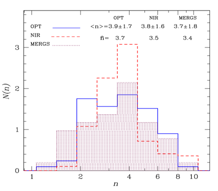
Figure 1 (top) shows the frequency distribution of $n$ for a set of observational data in optical wave bands (D01, La Barbera et al. 2005) and in the near-infrared ($K$) band [La Barbera et al 2005, Ravikumar et al. 2005 (R05)]. A total of 169 galaxies in the optical and 156 in the $K$ band were used here. The frequency distribution of 41 merger remnants observed in the $K$-band by Rothberg & Joseph (2004) are also indicated as a shaded histogram. The mean and standard deviations of these data sets are indicated, as well as their median.

Figure 1: (Top) Frequency distributions $N(n)$ for Sérsic index $n$ of a sample of early-type galaxies in the optical (opt, solid line) and near-infrared bands (nir, dashed line). (Bottom) Frequency distribution of our $N$-body remnants using both fitting intervals $I_{1}$ and $I_{2}$. The mean values and their standard deviations are indicated; below these, the median is indicated. $K$-band merger remnants (mergs) of Rothberg & Joseph (2004) correspond to the shaded histogram in both panels.

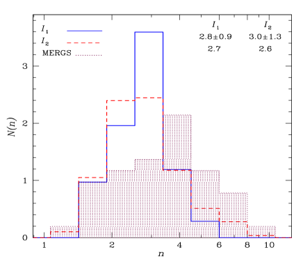
In Figure 1 (bottom) we show the distribution of $n$ for our merger remnants using the radial fitting intervals $I_{1}$ and $I_{2}$. The frequency distribution for our $N$-body remnants peak at a value $n\approx 3$ in both cases; although using $I_{2}$ it shows a somewhat broader distribution. For $I_{1}$ it is found that $n\in(1.5,5.3)$ and for $I_{2}$ that $n\!\in\!(1.4,9.5)$. These values are in good agreement with those found in intermediate mass ellipticals (e.g. Graham & Guzmán 2003, de Jong et al. 2004, Trujillo, Burkert & Bell 2004, Ellis et al. 2005), some brightest cluster galaxies (e.g. Graham et al. 1996), dwarf ellipticals (e.g. Binggeli & Jerjen 1998, Young & Currie 2001), and the local merger remnants of RJ04.

Our results using $I_{1}$, and no bulge, are consistent with the values found by NT and GGB for their models with a bulge in the progenitors. Furthermore, using interval $I_{2}$ lead to some values $n\!\approx\!9$. This does not seem to be due to the methodology in the computation of the surface density profiles. NT construct artificial images analogous to the observational procedure while GGB fit ellipses to isodensity contours, both considering a wide range in the radial fitting range, and obtaining similar ranges for $n$. It is likely that differences in the way models of the progenitors are set up be probably one of the reasons behind the differences with our results; see $\S$4.

Figure 2: Frequency distributions of $R_{\rm e}$ for observed early-type galaxies (top) and $N$-body remnants (bottom). Mean values and dispersion, along with medians, are indicated as in Figure 1. The same observational data sets considered in Figure 1 are used here.

3.1.2 Effective Radius

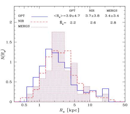
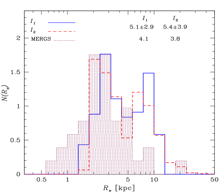
Figure 2 (top) shows the observed frequency distribution of effective radii $R_{\rm e}$ for the data considered in $\S$3.1.1 and that corresponding to our remnants (bottom). For the fitting radial range $I_{1}$ we obtain $R_{\rm e}\!\in\!(1.6,12.9)\,$kpc, and for $I_{2}$ we have $R_{\rm e}\!\in\!(1.6,34.5)\,$kpc. The average value of the observational data is about $4\,$kpc and for our remnants is about $5\,$kpc. It can be noticed that $R_{\rm e}$ shows a larger dispersion of values than the index $n$ depending on the fitting interval. This was also noticed by Binggeli & Jerjen (1998).

Our remnants have a lower bound of $R_{\rm e}\!\approx\!1.5\,$kpc, while the observational data considered here can reach smaller values $R_{\rm e}\!\mathrel{\hbox to0.0pt{\lower 3.0pt\hbox{$\mathchar 536\relax$}\hss}\raise 2.0pt\hbox{$\mathchar 318\relax$}}\!0.5\,$kpc. We are not able to reproduce the small values of $R_{\rm e}$ mainly because in our sample of initial conditions no pairs of small progenitors were included. On other hand, values of $R_{\rm e}\mathrel{\hbox to0.0pt{\lower 3.0pt\hbox{$\mathchar 536\relax$}\hss}\raise 2.0pt\hbox{$\mathchar 318\relax$}}10\,$kpc can be reproduced by our more massive remnants ($M01$ and $MM$); see Tables 2 and 3.

A unique comparison with the distribution of$R_{\rm e}$ values found by NT and GGB is not possible, since their models can be scaled to arbitrary physical units; a thing that is not possible here due to the way our disc galaxy progenitors were built up. Nonetheless, if we use the range of dimensionless values found by NT ($1\!<\!R_{\rm e}\!<\!1.7$) for systems classified as pure “bulges”, and use a length unit of $3.5\,$kpc (i.e., the radial scale-length of the Milky Way) to transform their results to physical units, we find that both results are consistent. Also, we obtain qualitatively the same behaviour as the one shown in their Figure 18 where a sharp cut at the lower-end of the distribution, as well as an extended tail at larger values.

Considering the observational values of $R_{\rm e}$ and those in our $N$-body remnants, we can establish with confidence that the simulations can reproduce quite well the observed range of values. Even some large values of $R_{\rm e}$ found in giant ellipticals (e.g., Graham et al. 1996) are reproduced.

3.2 Luminous Correlations

Several works (e.g. CCD93, D01, R05) have found a series of correlations among Sérsic parameters in early-type galaxies. We now turn to study some of these and compare them with the properties of our numerical remnants. Firstly, we consider two-dimensional correlations, and then turn to consider the so called Photometric Plane (PHP) [e.g. K00].

Figure 3: Sérsic index $n$ versus effective radius for the observational data of D01, R05, and RJ04. Genuine E galaxies from D01 are represented by a triangle ($\triangle$), while those classified as of an uncertain type by a star ($\star$). Merger remnants of RJ04 are open circles ($\circ$). Lines correspond to least-square fits. The values obtained, along with the coefficient of determination and rms in $\log n$ of the fit are indicated. The average results for our $N$-body remnants, using the radial range $I_{2}$, are shown with solid dots ($\bullet$) and points correspond to different projections of those numerical remnants.

3.2.1 Two Dimensional Correlations

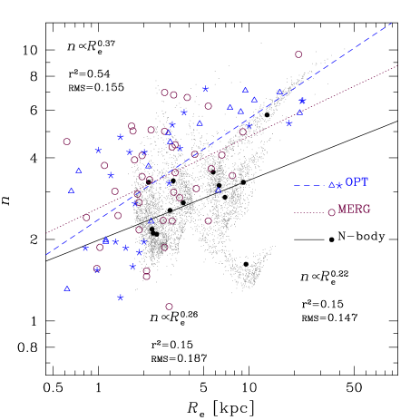
In the work of Caon et al. (1993) it was stated that a linear positive correlation between $n$ and $R_{\rm e}$ exists for early-type galaxies; they find that $n\propto R_{\rm e}^{0.52}$ for early-type galaxies in Virgo. A similar conclusion was reached by D’Onofrio, Capaccioli & Caon (1994) analysing galaxies in Fornax. Combining the data of both works one finds $n\propto R_{\rm e}^{0.50}$ with a Pearson’s linear correlation coefficient $r=0.72$. The statement of CCD93 that structure (as indicated by $n$) of an elliptical depends on its size $R_{\rm e}$ has been supported by the analysis of Trujillo, Graham & Caon (2001).

Figure 3 shows index $n$ against $R_{\rm e}$ for some of the data considered here, as well as the values obtained for our disc galaxy merger remnants. A linear least-square fit to the data of D01 leads to $n\propto R_{\rm e}^{0.37}$, and for RJ04 mergers $n\propto R_{\rm e}^{0.26}$; with linear correlation coefficients $r=0.73$ and $0.39$, respectively. A similar fit to our remnants yields $n\propto R_{\rm e}^{0.22}$ with $r=0.39$.

However, the observational data plotted in Figure 3 shows a large scatter around the assumed linear correlation; a fact already noticed by other authors (e.g. Trujillo et al. 2001). These fluctuations are quantified by considering the coefficient of determination ($r^{2}$) that measures the proportion of the variance of one variable that is predictable from the other (e.g. Ryan 1997). As indicated in Figure 3, the coefficients of determination are rather small, and the rms of the fits are large, so its is not clear that a true linear correlation exists between $\log n$ and $\log R_{\rm e}$.

We notice also that the $N$-body remnant $M05$, being the smallest one, has the second largest $n$ value in our simulations. These results lead us to state that there is no linear positive correlation between the “structure” and size of an elliptical. It seems that the values of $n$ and $R_{\rm e}$ are restricted by some physical mechanism to a finite region of the Sérsic parameter space; an option also indicated by Trujillo et al. (2001).

Figure 4: Sérsic index versus $\mu_{0}$ from observational data of D01 ($\triangle,\star$), RJ04 ($\circ$), R05 ($\times$). and $N$-body remnants mean values ($\bullet$) and their projected ones (points). Lines are the resulting scaling relations obtained from least-square fits. The coefficient of determination ($r^{2}$) and the rms are also indicated. For clarity, results from $N$-body remnants have been displaced by a constant value along the $\mu_{0}$–axis.

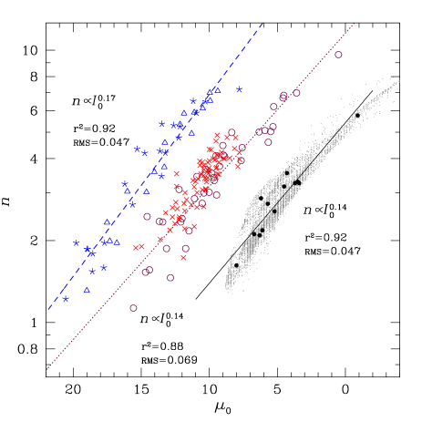
On other hand, a stronger observational correlation has been found between $n$ and the central brightness $\mu_{0}$ in ellipticals (e.g. K00, Graham & Guzmán 2003) and it appears to extend to dwarf ellipticals (e.g. Binggeli & Jerjen 1998, R05). In Figure 4 we plot these quantities for the observational data of D01, R05, RJ04, and for comparison our $N$-body remnants. A linear fit $\log n$–$\mu_{0}$ to these data leads to $n\propto I_{0}^{0.17}$ for D01, $n\propto I_{0}^{0.14}$ for both RJ04 and the ellipticals in R05, and $n\propto I_{0}^{0.14}$ for our merger remnants. All fits have $r^{2}\mathrel{\hbox to0.0pt{\lower 3.0pt\hbox{$\mathchar 536\relax$}\hss}\raise 2.0pt\hbox{$\mathchar 318\relax$}}0.9$ and an rms $\mathrel{\hbox to0.0pt{\lower 3.0pt\hbox{$\mathchar 536\relax$}\hss}\raise 2.0pt\hbox{$\mathchar 316\relax$}}0.07$, that lead us to conclude that $\log n$–$\mu_{0}$ is a true linear correlation, at least for the range of $n$ values considered.

As shown, the numerical remnants presented here are able to reproduce very well the $\log n$–$\mu_{0}$ correlation and its tightness. We recall that we have assumed a constant mass-to-light ratio to convert $\Sigma_{0}$ to $I_{0}$ in order to compare with observations. Hence, it appears that at least in the range of masses of our remnants (Table 1), there is no need to assume a dependence of the mass-to-light ratio dependence with mass (or luminosity) to reproduce the observations.

3.2.2 The Photometric “Plane”

Several authors [e.g. K00, Graham 2002, Khosroshahi et al. 2004 (K04), La Barbera et al. 2005, R05] have found that Sérsic parameters $\{n,R_{\rm e},\mu_{0}\}$ of early-type galaxies define a plane in log-space of the form

$$\log n=a\log R_{\rm e}+b\,\mu_{0}+c\,,$$ (6)

which is termed the “photometric plane” (PHP). Some authors instead of $\mu_{0}$ use the mean effective brightness $\langle\mu\rangle_{\rm e}$ (e.g. Graham 2002, La Barbera et al. 2005). The different 2D correlations of $\S$3.2.1 can be considered then projections of the PHP.

We have computed, by a linear-square fit procedure, the coefficients of this PHP for our remnants under the assumption of a constant mass-to-light ratio. Since we find that using $\langle\mu\rangle_{\rm e}$ leads to about twice the rms in $\log n$ than using $\mu_{0}$, we restrict ourselves to an expression of the form (6).

Table 4: Photometric Plane coefficients

id	$a$	$-b$	$c$	rmsn
K00	$0.17\pm 0.03$	$0.069\pm 0.007$	$1.2\pm 0.1$	0.04
D01	$0.09\pm 0.02$	$0.058\pm 0.004$	$1.3\pm 0.1$	0.06
K04	$0.21\pm 0.09$	$0.074\pm 0.013$	$1.7\pm 0.3$	0.13
R05E	$0.15\pm 0.02$	$0.066\pm 0.003$	$1.1\pm 0.0$	0.04
R05dE	$0.16\pm 0.04$	$0.082\pm 0.004$	$1.6\pm 0.1$	0.07
RJ04	$0.11\pm 0.04$	$0.054\pm 0.004$	$1.0\pm 0.0$	0.06
M($I_{1}$)	$0.05\pm 0.00$	$0.057\pm 0.001$	$-1.0\pm 0.0$	0.05
M($I_{2}$)	$0.05\pm 0.01$	$0.057\pm 0.001$	$-1.0\pm 0.0$	0.05

Figure 5: Representation of the photometric plane (PHP) for the same observational data of Figure 4, and for our numerical remnants. Symbols are as in Figure 4. The $x$-axis is defined here with the values obtained from D01 data. Scalings $n\propto R_{\rm e}^{\alpha}I_{0}^{\beta}$ are indicated, along with the rms of the linear fit. $N$-body remnants have been displaced a constant term.

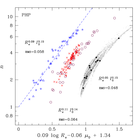
In Table 4 we list the values of the coefficients of (6) found in the works of K00, K04, RJ04, the elliptical and dwarf ellipticals of R05, and those we obtain from the data of D01. Also shown are the coefficients found for our merger remnants for both fitting radial intervals $I_{1}$ and $I_{2}$; M($I_{1}$) and M($I_{2}$), respectively. In Figure 5 we plot the PHP from these data, using for illustrative purposes the values from the data of D01 to define the abscissa axis.

The remnants’ coefficient $b$ in (6), associated with $\mu_{0}$, is rather consistent with the observed ones, aside of those found in dEs (R05). The coefficient $a$, associated with $R_{\rm e}$, is less well reproduced. This is not surprising taking into account the large dispersion in the $n$–$R_{\rm e}$ relation (see Figure 3). As several authors have pointed out (e.g. K00, K04, R05) a slight curvature towards small values of $n$ is observed, a feature that tends to be reproduced here by the effect of merger $M11$ that has $n\!\approx\!1.5$. The rms is similar for both the observational data and our simulations. The best overall agreement is obtained with the data of D01.

We consider that our $a$ and $b$ values are rather consistent with the whole set of values listed in Table 4, and that the numerical remnants are able to reproduce the PHP. In $\S$4 we argue that the PHP is not really a plane, but a “pseudo-plane” with a small curvature at low values of $n$ due to the intrinsic properties of Sérsic model.

3.3 Dark Haloes

Dark haloes in cosmological simulations are started to being described by a 3D Sérsic function (Merritt et al. 2005, Prada et al. 2005, Graham et al. 2005), of the form

$$\rho(r)=\rho_{0}\exp[-d_{n}(r/r_{\rm e})^{1/n}]$$ (7)

with $r$ being the spatial radius, $r_{\rm e}$ a 3D “effective radius”, and $d_{n}\approx 3n-1/3+0.005/n^{2}$ (Graham et al. 2005). It has been found that (7) provides a better fit to dark haloes than the typical NFW or M99 (Moore et al. 1999) density profiles. Sérsic indices of about $6$, with a scatter of $\approx 1$, are found for the cosmological dark haloes.

Table 5: Dark haloes 3D Sérsic fits

id	$n$	$r_{\rm e}$	$\log\rho_{0}$		rms
		[kpc]	[M${}_{\odot}/{\rm kpc}^{3}$]
$M01$	3.3	86.7	9.08		0.05
$M02$	3.5	28.4	9.81		0.03
$M03$	4.5	26.5	10.90		0.04
$M04$	4.0	42.1	10.17		0.08
$M05$	4.3	20.4	10.93		0.06
$M06$	4.4	25.2	10.88		0.05
$M07$	3.9	23.0	10.32		0.05
$M08$	3.8	28.9	9.99		0.05
$M09$	4.5	29.0	10.92		0.07
$M10$	4.0	31.9	10.24		0.12
$M11$	3.7	41.3	10.03		0.06
$M12$	3.3	39.5	9.38		0.05
$MM$	3.0	82.6	8.78		0.04

Figure 6: (Top) Fitted 3D Sérsic profiles (7) to the dark haloes of our remnants. (Bottom) Logarithmic residuals of the fits.

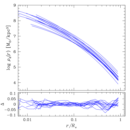
We have fitted 3D Sérsic profiles (7) to the dark haloes of our remnants. The radial range of the fit was from the convergence radius $r_{\rm c}$ (e.g. Power et al. 2003) to the dynamical virial radius of the remnant (Table 1). However, instead of using the orbital period at the $r_{200}$ radius to determine $r_{\rm c}$ as done in cosmological simulations, we used the orbital period at the virial radius.

In Figure 6 we display the fitted 3D Sérsic profiles, along with their residuals. In Table 5 the values of the 3D Sérsic parameters are listed for each remnant, as well as the corresponding rms. It can be seen that the 3D Sérsic profile (7) is a very good representation of the density distribution up to the virial radius of each remnant. This is in concordance with the behaviour of the 3D Sérsic profile for characterising cosmological haloes.

The haloes of the $N$-body remnants have a mean 3D Sérsic index $\langle n\rangle\!=\!3.9\pm 0.5$; the uncertainty being the standard deviation. A value that is lower than that found for cosmological haloes. However, it is consistent with the mean value of the dark haloes of the progenitors $\langle n\rangle\!=\!3.7\pm 0.3$; as expected from the preservation of the cuspyness of dark haloes in mergers (e.g. Boylan-Kolchin & Ma 2004, Aceves & Velázquez 2006, Kazantzidis, Zentner & Kravtsov 2006).

Figure 7: Relations between different physical quantities of the dark matter haloes obtained from a Sérsic de-projected profile.

Differences in results are expected since the outer radius of the fits are not the same; we use a dynamical virial radius while for cosmological haloes the fits are done up to $r_{200}$ or further out (e.g. Prada et al. 2005). It should be noticed that Sérsic fits (7) by Graham et al. (2005) have values for $r_{\rm e}$ (see their Table 1) in some cases larger than their cosmological virial radius; these last ones listed in Table 1 of Diemand, Moore & Stadel (2004). For example, their haloes G02 and G03 have $r_{\rm e}\!=\!391.4$ kpc and 405.6 kpc, respectively, while their virial radii are $337\,$kpc and $299\,$kpc; halo B09 shows even a more larger discrepancy. Unfortunately, they do not provide their numerical half-mass radii to make a direct comparison with the values $r_{\rm e}$ they obtained. Also, Merritt et al. (2005) and Prada et al. (2005) do not provide the fitted values $r_{\rm e}$ and the numerical half-mass radii. This makes uncertain any comparison of our results with these works.

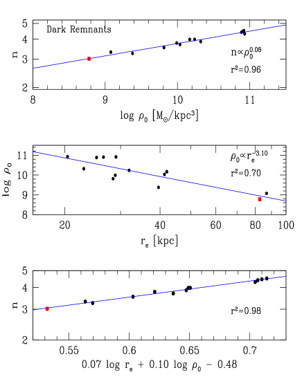
Figure 7 shows different relations among the 3D Sérsic parameters for the haloes of our remnants: $n$–$\rho_{0}$ and $\rho_{0}$–$r_{\rm e}$, and in analogy to the PHP we have constructed a 3D dark Sérsic plane (DSP). We find, assuming a log-linear correlation, that $n\propto\rho_{0}^{0.08}$ and $\rho_{0}\propto r_{\rm e}^{-3.10}$ with coefficients of determination $0.96$ and $0.70$, respectively. This indicates that $n$–$\rho_{0}$ can be considered with confidence a true log-linear positive correlation, as its was in the corresponding 2D case, but we do not deem on the same level $\rho_{0}$–$r_{\rm e}$. The DSP found for the remnants is

$$\log n\!=\!(0.07\pm 0.02)\log r_{\rm e}-(0.04\pm 0.00)\bar{\mu}_{0}-(0.48\pm 0.07)\;$$ (8)

where $\bar{\mu}_{0}\!=\!-2.5\log\rho_{0}$. This turns out to be a very tight correlation, with a coefficient of determination of $0.98$ and rms of $0.007$, for the range of haloes masses considered in our simulations (see Table 1).

4 Final Remarks and Conclusions

The results found here, as well as those of NT and GGB, show that the merger scenario is capable of reproducing the Sérsic properties of observed elliptical galaxies. This work shows, however, that the presence of a “primordial” bulge in the progenitors is not necessary to satisfy, for example, the observed values of the shape parameter $n$; as was suggested by NT and GGB.

It is likely that the different results with NT and GGB have their origin on the initial properties of the progenitors; in particular, their dark matter distribution. We have used cuspy (NFW-type) dark haloes in contrast to those used by NT (pseudo-isothermal) and GGB (Lowered Evans) that have a constant density core. It is probable that the higher concentration of dark matter used here, affected the distribution of luminous matter in a way to increase the index $n$ which is correlated with the luminous concentration (Trujillo et al. 2001). Other initial conditions of the progenitors and of the encounters such as energy and angular momentum, both intrinsic and orbital, may have played a role in the final concentration of luminous matter of the remnants, as indicated by the index $n$. A systematic study of the way different dynamical elements determine the Sérsic index is, however, beyond the scope of the present work.

We have shown that haloes of remnants define a tight dark Sérsic plane (DSP) analogous to that of the luminous matter and with less dispersion. No indication of curvature is present, at difference to what is noted in the PHP at low values of $n$. We argue here that this curvature is real and is related to an intrinsic property of a Sérsic profile. Consider the expression for the total luminous matter associated with a Sérsic profile (3). This can be written in log-space as

$$\log L_{\rm T}=\log n-0.4\,\mu_{0}+2\log R_{\rm e}+\log f_{2}(n)$$ (9)

with the “form factor” $f_{2}(n)=2\pi\Gamma(2n)/b^{2n}$. A given set of galaxies with equal $L_{\rm T}$ and different Sérsic parameters would define an exact log-plane, except for the presence of the $\log f_{2}(n)$ term. In the 3D Sérsic function (7) the analogous form factor is $f_{3}(n)=4\pi\Gamma(3n)/d^{3n}$. These non-constant terms introduce a systematic change in a PHP-like expression. The importance of the form factor is larger for values $n\mathrel{\hbox to0.0pt{\lower 3.0pt\hbox{$\mathchar 536\relax$}\hss}\raise 2.0pt\hbox{$\mathchar 316\relax$}}1$ and smaller for $n\mathrel{\hbox to0.0pt{\lower 3.0pt\hbox{$\mathchar 536\relax$}\hss}\raise 2.0pt\hbox{$\mathchar 318\relax$}}1$; both $f_{2}(n)$ and $f_{3}(n)$ are shown in Figure 8. Thus, the form factor of the Sérsic model determines the curvature observed in the PHP. This explains why no curvature is found by La Barbera et al. (2005) whose galaxies show $n\mathrel{\hbox to0.0pt{\lower 3.0pt\hbox{$\mathchar 536\relax$}\hss}\raise 2.0pt\hbox{$\mathchar 318\relax$}}2$, but this can be seen in dwarf ellipticals with several values of $n\mathrel{\hbox to0.0pt{\lower 3.0pt\hbox{$\mathchar 536\relax$}\hss}\raise 2.0pt\hbox{$\mathchar 316\relax$}}1$ (K04). Also, the DSP does not show such curvature since $n\mathrel{\hbox to0.0pt{\lower 3.0pt\hbox{$\mathchar 536\relax$}\hss}\raise 2.0pt\hbox{$\mathchar 318\relax$}}3$ (see Figure 7). Furthermore, the dispersion about these “planes” is determined by the luminosity or dark mass range of the galaxy sample.

Figure 8: Form factor $f_{2}(n)$ in equation (9) contributing to the observed curvature of the photometric “plane” at low values of $n$; for an ensemble of equal total-luminous projected mass galaxies. An analogous $f_{3}(n)$ for a 3D distribution is also plotted.

It remains to study the central phase-space densities of the remnants, to see if they are consistent with the estimates for ellipticals (e.g. Carlberg 1986), and to analyse their kinematical properties with those observed in elliptical galaxies. We plan to study these topics in a future work. In summary, our main conclusions are as follows:

1. Collision-less mergers of pure disc galaxies yield values and distributions of Sérsic parameters consistent with those observed for bona fide ellipticals. The existence of a bulge in merging spirals does not appear to be a necessary condition on grounds of Sérsic properties of the remnants.

2. The suggested positive log-linear correlation between the size ($R_{\rm e}$) and structure ($n$) in ellipticals is not supported. However, the strong $\log~{}n$–$\mu_{0}$ linear correlation found in observational studies is supported by our merger simulations. On other hand, the PHP is fairly well reproduced. For these results a constant mass-to-light ratio is assumed.

3. The final dark haloes of remnants show values of $n\approx 4$ lower than those found in cosmological simulations $n\approx 6$. The difference may be attributable to the non-equivalence outer radius, where the dynamical virial radius was used in our case to carry out the fitting by a Sérsic profile. Haloes define a tight Dark Sérsic Plane (DSP) in three dimensions, with no indication of curvature at the level of the smaller $n$ obtained.

4. The curvature observed in the PHP at low values of $n$ is an intrinsic manifestation of the properties of Sérsic model, due to the presence of a non-constant term dependent of $n$.

Appendix

We briefly discuss here the effect of the radial interval on the fitting process of a Sérsic profile to a mass distribution. To do this we generate exact Sérsic profiles with $R_{\rm e}\!=\!1$, $L_{\rm T}\!=\!1$, and $n=2,4,8$. Also, random fractional errors $\leq\{1,10,20\}$% are introduced. The radial fitting interval is chosen as follows. A random inner point $\xi$ is selected from the interval $[0.03,0.5]R_{\rm e}$ while the outer radius, $\eta$, is randomly generated from the interval $[R_{70},R_{95}]$; where $R_{70}$ and $R_{95}$ correspond to the radii containing 70% and 95% percent of the projected mass. These two points define our radial fitting interval $[\xi,\eta]$. To corroborate the importance the importance of the underlying mass distribution we use also a Hernquist (1990) mass model with an without errors.

Sérsic Distribution

Table 6 lists the mean values of $\{n,R_{\rm e},\mu_{0}\}$ obtained from fitting 1000 Monte Carlo experiments for three Sérsic models with errors as indicated above. Each line lists, in order of the ascending error introduced to the theoretical Sérsic profile, the parameters recovered from the fit inside the random interval $[\xi,\eta]$. The standard deviation for each quantity is provided.

These results show that the determination of Sérsic parameters is very robust, for errors $\mathrel{\hbox to0.0pt{\lower 3.0pt\hbox{$\mathchar 536\relax$}\hss}\raise 2.0pt\hbox{$\mathchar 316\relax$}}10$%, against the size of the fitting region. As the error in the ideal Sérsic distribution increases the dispersion grows. This is more clearly appreciated for index $n$. In the limit of zero error, even for a random radial fitting interval, the model parameters are recovered exactly. For this case, we conclude that the radial fitting range does not has an important effect on Sérsic fitted parameters.

Table 6: Sérsic fits.

$n_{\rm{true}}$	$n$	$R_{\rm e}$	$-\mu_{0}$
2	$2.000\pm 0.015$	$1.000\pm 0.003$	$\hphantom{0}0.956\pm\hphantom{0}0.030$
	$2.014\pm 0.162$	$1.002\pm 0.031$	$\hphantom{0}0.981\pm\hphantom{0}0.319$
	$2.061\pm 0.418$	$1.009\pm 0.082$	$\hphantom{0}1.067\pm\hphantom{0}0.819$
4	$4.001\pm 0.037$	$1.000\pm 0.004$	$\hphantom{0}4.940\pm\hphantom{0}0.080$
	$4.041\pm 0.408$	$1.001\pm 0.043$	$\hphantom{0}5.026\pm\hphantom{0}0.876$
	$4.222\pm 1.749$	$1.010\pm 0.139$	$\hphantom{0}5.407\pm\hphantom{0}3.719$
8	$8.002\pm 0.087$	$0.999\pm 0.007$	$13.261\pm\hphantom{0}0.196$
	$8.119\pm 1.042$	$0.998\pm 0.071$	$13.521\pm\hphantom{0}2.316$
	$8.663\pm 4.776$	$1.006\pm 0.251$	$14.719\pm 10.407$

Hernquist Distribution

We now consider that the case where the underlying mass distribution follows a Hernquist model. Here, $R_{\rm hl}$ denotes its theoretical projected half-light (mass) radius. It is found that in the fitting interval $[0.03,2.79]R_{\rm hl}$ , the underlying Hernquist’s profile is fitted by a Sérsic profile with index $n=2.6$ and $R_{\rm e}=0.82$ in agreement with NT. For a radial fitting interval of $[0.03,14.5]R_{\rm hl}$ we find that $n\!=\!3.67$ and $R_{\rm e}\!=\!1.10$. This indicates that the process of fitting a Sérsic profile is far more sensitive when the underlying mass distribution does not follows a Sérsic one.

The above was already noted by Boylan-Kolchin, Ma & Quataert (2005), where a systematic change in Sérsic parameters was found when trying to fit a Hernquist profile. In Figure 9 (left) we reproduce this systematic effect, for the Sérsic index $n$, $R_{\rm e}$, and the mean effective surface brightness $\langle I_{\rm e}\rangle$. If a random error $\leq 10$% is introduced the trend is preserved but a large dispersion results; especially as the inner radius of radial interval of the fit is increased.

Figure 9: Dependence of Sérsic parameters $\left\{n,R_{\rm e},\langle I\rangle_{\rm e}\right\}$ with the fitting interval for an underlying Hernquist profile. (Left) Ideal Hernquist profile. (Right) A random fractional error $\leq 10$% is introduced to Hernquist profile. Each point corresponds to a different Monte Carlo realisation of the profile. Symbols represent different inner points to carry out the fittings in terms of the theoretical half-light radius $R_{\rm hl}$ of Hernquist profile.

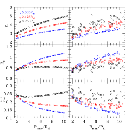
Figure 10 shows the distribution of fitted values with no error (solid line) and with a random error $\leq 10$% (dashed line) for an underlying Hernquist profile where the radial interval was obtained from $\xi\in[0.06,0.50]R_{\rm hl}$ and $\eta\in[\eta_{70},\eta_{95}]$. The mean and standard deviations of the distribution are indicated. For comparison, the histogram of values corresponding to a Sérsic model with $n=4$ with a random error $\leq 10$% is also shown (dotted line); see Table 6, second line in the entry for $n=4$.

Figure 10: Frequency distributions of fitted Sérsic parameters to a Hernquist profile. The radial range of the fit is similar to the interval $I_{2}$ used for our $N$-body remnants. Solid lines is an ideal Hernquist model, while the dashed line corresponds to the addition of a random error $\leq 10$%. The dotted line corresponds to a Sérsic distribution with $n\!=\!4$ and random error $\leq 10$%, shown for comparison. Mean values and standard deviations are indicated.

From the above results, it follows that when the underlying mass distribution is not of a Sérsic type, the fitted values have a rather large dispersion even in the presence of no error. In particular, higher values of the index $n$ are obtained for different radial ranges of the fit. In order to have a confident estimate of $n$, and other parameters, one has to sample rather deep inside and outside the luminous (mass) distribution; from about $0.1$ to $6\,R_{\rm hl}$.

In practise, for example, sampling very near the centre of a galaxy may pose problems due to resolution effects. This is a particular problem for observations of galaxies at different redshifts, using the same angular resolution but representing different physical scales, and can lead to uncertain Sérsic parameters.

References

- [1] Aceves H., Velázquez H., 2005, RMxAA, 41, 523
- [2] Aceves H., Velázquez H., 2006, RMxAA, 42, 23 (astro -ph/0506290)
- [Baum(1990)] Baum W. A. 1990, ASP Conf. Ser. 10: Evolution of the Universe of Galaxies, 10, 119
- [\citeauthoryearBernardi et al.2003] Bernardi M., et al., 2003, AJ, 125, 1866
- [Binggeli & Jerjen(1998)] Binggeli B., Jerjen H. 1998, A& A, 333, 17
- [Bower et al.(2005)] Bower R. G., Benson A. J., Malbon R., Helly J. C., Frenk C. S., Baugh C. M., Cole S., Lacey C. G. 2005, astro-ph/0511338
- [3] Boylan-Kolchin M., Ma C.-P., 2004, MNRAS, 349, 1117
- [4] Boylan-Kolchin M., Ma C.-P., Quataert E. 2005, MNRAS, 362, 184
- [Caon et al.(1993)] Caon N., Capaccioli M., D’Onofrio M. 1993, MNRAS, 265, 1013 (CCD93)
- [\citeauthoryearCapaccioli et al.1992] Capaccioli M., Caon N., D’Onofrio M., 1992, MNRAS, 259, 3223
- [Carlberg(1986)] Carlberg R. G. 1986, ApJ, 310, 593
- [5] Ciotti L., Bertin G., 1999, A&A, 352, 447 L13
- [Cole et al.(2000)] Cole S., Lacey C. G., Baugh C. M., Frenk C. S. 2000, MNRAS, 319, 168
- [de Jong et al.(2004)] de Jong R. S., Simard L., Davies R. L., Saglia R. P., Burstein D., Colless M., McMahan R., Wegner G. 2004, MNRAS, 355, 1155
- [6] de Vaucouleurs G. 1948, Ann. d’Astrophys., 11, 247
- [De Lucia et al.(2005)] De Lucia G., Springel V., White S. D. M., Croton D., Kauffmann G. 2005, astro-ph/0509725
- [7] D’Onofrio M., Capaccioli M., Caon N. 1994, MNRAS, 271, 523
- [D’Onofrio(2001)] D’Onofrio M. 2001, MNRAS, 326, 1517 (D01)
- [8] Diemand J., Moore B., Stadel J., 2004, MNRAS, 352, 535
- [\citeauthoryearDjorgovski & Davis1987] Djorgovski S., Davis M., 1987, ApJ, 313, 59
- [9] Dressler A., Lynden-Bell D., Burstein D., Davies R. L., Faber S. M., Terlevich R. J., Wegner G., 1987, 313, 42
- [10] Efstathiou G., Lake G., Negroponte J., 1982, MNRAS, 199, 1069
- [Ellis et al.(2005)] Ellis S. C., Driver S. P., Allen P. D., Liske J., Bland-Hawthorn J., De Propris R. 2005, MNRAS, 363, 1257
- [\citeauthoryearFaber & Jackson1976] Faber S. M., Jackson R. E., 1976, ApJ., 204, 668
- [11] González-García A. C., Balcels M., 2005, MNRAS, 357, 753 (GGB)
- [Graham (2002)] Graham A. W., 2002, MNRAS, 334, 859
- [Graham et al. (1996)] Graham A., Lauer T. R., Colless M., Postman M., 1996, ApJ, 465, 534
- [Graham & Colless(1997)] Graham A., Colless M. 1997, MNRAS, 287, 221
- [Graham & Guzmán(2003)] Graham A. W., Guzmán R. 2003, AJ, 125, 2936
- [12] Graham A. W., Driver S. P., 2005, PASA, 22, 118
- [13] Graham A. W., Merritt D., Moore B., Diemand J., Tzerzic B., 2005 astro-ph/0509417
- [Hernquist(1990)] Hernquist L. 1990, ApJ, 356, 359
- [Kaviraj et al.(2006)] Kaviraj S., et al. 2006, astro-ph/0601029
- [14] Kazantzidis S., Zentner A. R., Kravtsov A. V., 2006, astro-ph/0510583
- [15] Kelson D. D., Illingworth G. D., van Dokkum P. G., Franx M., 2000, 531, 137
- [16] Khosroshahi H. G., Wadadekar Y., Kembhavi A., Mobasher B., 2000, ApJ, 531, L103 (K00)
- [Khosroshahi et al.(2004)] Khosroshahi H. G., Raychaudhury S., Ponman T. J., Miles T. A., Forbes D. A. 2004, MNRAS, 349, 527 (K04)
- [\citeauthoryearKormendy1977] Kormendy J., 1977, ApJ., 218, 333
- [La Barbera et al.(2005)] La Barbera F., Covone G., Busarello G., Capaccioli M., Haines C. P., Mercurio A., Merluzzi P. 2005, MNRAS, 358, 1116
- [Merritt et al.(2005)] Merritt D., Navarro J. F., Ludlow A., Jenkins A., 2005, ApJ, 624, L85
- [Meza et al.(2003)] Meza A., Navarro J. F., Steinmetz M., Eke V. R. 2003, ApJ, 590, 619
- [Moore et al.(1999)] Moore B., Quinn T., Governato F., Stadel J., Lake G. 1999, MNRAS, 310, 1147 (M99)
- [\citeauthoryearNaab & Burkert2003] Naab T., Burkert A. 2003, ApJ, 597, 893
- [17] Naab T., Trujillo I., 2005, astro-ph/0508362 (NT)
- [Naab et al.(2005)] Naab T., Johansson P. H., Efstathiou G., Ostriker J. P. 2005, astro-ph/0512235
- [Navarro et al.(1997)] Navarro J. F., Frenk C. S., White S. D. M. 1997, ApJ, 490, 493 (NFW)
- [18] Navarro J. F., et al., 2004, MNRAS, 349, 1039
- [Peebles(2002)] Peebles, P. J. E. 2002, ASP Conf. Ser. 283: A New Era in Cosmology, 283, 351
- [Power et al.(2003)] Power C., Navarro J. F., Jenkins A., Frenk C. S., White S. D. M., Springel V., Stadel J., Quinn T. 2003, MNRAS, 338, 14
- [19] Press W. H., Teukolsy S. A., Vetterling W. T., Flannery B. P., 1992, Numerical Recipes: The Art of Scientific Computing. Cambridge Univ. Press, New York
- [20] Prada F., Klypin A. A., Simonneau E., Betancort-Rijo J., Patiri S., Gottloeber S., Sánchez-Conde M. A., 2005, astro-ph/0506432
- [Prugniel & Simien(1997)] Prugniel P., Simien F. 1997, A&A, 321, 111
- [21] Ravikumar C. D., Barway S., Kembhavi, Mobasher B., Kuriakose V. C., astro-ph/0509391 (R05)
- [22] Rothberg B., Joseph, R. D. 2004, AJ, 128, 2098 (RJ04)
- [Rothberg & Joseph(2006)] Rothberg B., Joseph R. D. 2006, AJ, 131, 185
- [23] Ryan T. P., 1997, Modern Regression Methods, Wiley, NY
- [Schweizer(1998)] Schweizer F. 1998, Saas-Fee Advanced Course 26: Galaxies: Interactions and Induced Star Formation, 105
- [\citeauthoryearSérsic1968] Sérsic J. L., 1968, Atlas de Galaxias Australes. Córdoba, Argentina: Observatorio Astronómico
- [Shen et al.(2002)] Shen S., Mo H. J., Shu C. 2002, MNRAS, 331, 259
- [Springel et al.(2001)] Springel V., Yoshida N., White S. D. M. 2001, New Astronomy, 6, 79
- [24] Struck C., 2005, astro-ph/0511335
- [Tantalo & Chiosi(2004)] Tantalo, R., & Chiosi, C. 2004, MNRAS, 353, 405
- [Toomre(1977)] Toomre A. 1977, Evolution of Galaxies and Stellar Populations. Edited by Beatrice M. Tinsley and Richard B. Larson. New Haven: Yale University Observatory, p.401
- [25] Trujillo I., Graham A. W., Caon N., 2001, MNRAS, 326, 869
- [Trujillo et al.(2004)] Trujillo I., Burkert A., Bell E. F. 2004, ApJ, 600, L39
- [Trujillo et al.(2004)] Trujillo I., Erwin P., Asensio Ramos A., Graham A. W. 2004, AJ, 127, 1917
- [26] Young C K., Currie M. J., 2001, A&A, 369, 736