Understanding the origin of CMB constraints on Dark Energy

Abstract

We study the observational constraints of CMB temperature and polarization anisotropies on models of dark energy, with special focus on models with variation in properties of dark energy with time. We demonstrate that the key constraint from CMB observations arises from the location of acoustic peaks. An additional constraint arises from the limits on $\Omega_{NR}$ from the relative amplitudes of acoustic peaks. Further, we show that the distance to the last scattering surface is not how the CMB observations constrain the combination of parameters for models of dark energy. We also use constraints from Supernova observations and show that unlike the Gold and Silver samples, the SNLS sample prefers a region of parameter space that has a significant overlap with the region preferred by the CMB observations. This is a verification of a conjecture made by us in an earlier work (Jassal, Bagla, & Padmanabhan, 2005a). We discuss combined constraints from WMAP5 and SNLS observations. We find that models with $w\simeq-1$ are preferred for models with a constant equation of state parameters. In case of models with a time varying dark energy, we show that constraints on evolution of dark energy density are almost independent of the type of variation assumed for the equation of state parameter. This makes it easy to get approximate constraints from CMB observations on arbitrary models of dark energy. Constraints on models with a time varying dark energy are predominantly due to CMB observations, with Supernova constraints playing only a marginal role.

1 Introduction

Observational evidence for accelerated expansion in the universe has been growing in the last two decades (Ostriker & Steinhardt, 1995; Bagla, Padmanabhan & Narlikar, 1996; Efstathiou, Sutherland & Maddox, 1990). Independent confirmation using observations of high redshift supernovae (Garnavich et al., 1998; Perlmutter et al., 1999; Tonry et al., 2003; Barris et al., 2004; Riess et al., 2004; Astier et al., 2005) has made this result more acceptable to the community. Using these observations along with observations of cosmic microwave background radiation (CMB) (Melchiorri et al., 2000; Spergel et al., 2003; Komatsu et al., 2009) and large scale structure (Percival et al., 2007), we can construct a “concordance” model for cosmology and study variations around it (e.g., see Dunkley et al. (2008); Komatsu et al. (2009); Bridle et al. (2003); Tegmark et al. (2004); for an overview of our current understanding, see Padmanabhan (2005b, d, e)).

Observations indicate that the dominant component of energy density — called dark energy — should have an equation of state parameter $w\equiv P/\rho<-1/3$ for the universe to undergo accelerated expansion. Indeed, present day observations require $w\simeq-1$. The cosmological constant is the simplest explanation for accelerated expansion (Weinberg, 1989; Carroll, Press, & Turner, 1992; Sahni & Starobinsky, 2000; Padmanabhan, 2003; Peebles & Ratra, 2003; Ellis, 2003; Padmanabhan, 2005a; Perivolaropoulos, 2005; Copeland, Sami & Tsujikawa, 2006) and it is known to be consistent with observations. In order to avoid theoretical problems related to cosmological constant (Weinberg, 1989; Carroll, Press, & Turner, 1992), many other scenarios have been investigated: these include quintessence (Steinhardt, 2003; de la Macorra & Piccinelli, 2000; Urena-Lopez & Matos, 2000; Gonzalez-Diaz, 2002; de Ritis & Marino, 2001; Sen & Seshadri, 2003; Rubano & Scudellaro, 2002; Bludman & Roos, 2002), k-essence (Armendariz-Picon, Mukhanov, & Steinhardt, 2001; Chiba, 2002; Malquarti et al., 2003; Chimento & Feinstein, 2004; Scherrer, 2004), tachyon field (Sen, 2003; Padmanabhan, 2002; Bagla, Jassal & Padmanabhan, 2003; Jassal, 2004; Aguirregabiria & Lazkoz, 2004; Gorini et al., 2004; Gibbons, 2003; Kim, Kim & Kim, 2003; Shiu & Wasserman, 2002; Choudhury et al., 2002; Frolov, Kofman & Starobinsky, 2002; Gibbons, 2002), chaplygin gas and its generalisations (Gorini et al., 2001; Bento, Bertolami & Sen, 2002; Dev, Jain & Alcaniz, 2003; Sen & Scherrer, 2005), phantom fields (Caldwell, 2002; Hao & Li, 2003; Gibbons, 2003; Nojiri & Odinstov, 2003; Onemli & Woodard, 2002; Carroll, Hoffman & Trodden, 2003; Singh, Sami & Dadhich, 2003; Frampton, 2003; Gonzalez-Diaz, 2003; Dabrowski, Stachowiak & Szydlowski, 2003; Elizalde, Nojiri, & Odintsov, 2004; Nojiri, Odintsov, & Tsujikawa, 2005; Briscese et al., 2007; Bronnikov, Fabris, & Gonçalves, 2007; Bronnikov & Starobinsky, 2007), branes (Uzawa & Soda, 2001; Jassal, 2003; Burgess, 2003; Milton, 2003; Gonzalez-Diaz, 2000; Sahni & Shtanov, 2003) and many others (Holman & Naidu, 2004; Onemli & Woodard, 2004; Padmanabhan, 2005c, 2002; Andrianov, Cannata & Kamenshchik, 2005; Lazkoz, Neseseris & Perivolaropoulos, 2005; Cognola, Elizalde, Nojiri, Odinstov & Zerbini, 2006; Ren & Meng, 2005; Polarski & Ranquet, 2005; Sola & Stefancic, 2005; Das, Banerjee & Dadhich, 2005; Apostolopoulos & Tetradis, 2006; Arianto et al., 2007; Sahni, Shafieloo & Starobinsky, 2008) In these models one can have $w\neq-1$ and in general $w$ varies with redshift. For references to papers that discuss specific models, the reader may consult one of the many reviews (Sahni & Starobinsky, 2000; Padmanabhan, 2003; Peebles & Ratra, 2003; Ellis, 2003; Padmanabhan, 2005a; Alcaniz, 2006). Even though these models have been proposed to overcome the fine tuning problem for cosmological constant, most models require similar fine tuning of parameter(s) to be consistent with observations. Nevertheless, they raise the possibility of $w(z)$ evolving with time (or it being different from $-1$), which can be tested by observations.

Given that $w$ for dark energy should be smaller than $-1/3$ for the Universe to undergo accelerated expansion, the energy density of this component changes at a much slower rate than that of matter and radiation. (Indeed, $w=-1$ for cosmological constant and in this case the energy density is a constant.) Unless $w$ is a rapidly varying function of redshift and becomes $w\sim 0$ at ($z\sim 1$), the energy density of dark energy should be negligible at high redshifts ($z\gg 1$) compared to that of non-relativistic matter. If dark energy evolves in a manner such that its energy density is comparable to, or greater than the matter density in the universe at high redshifts then the basic structure of the cosmological model needs to be modified. We do not consider such models, instead we confine our attention to constraints on dark energy in realistic models and choose observations which are sensitive to evolution of $w(z)$ at redshifts $z\leq 1$.

Supernova observations permit a large variation in the equation of state (Alam et al., 2004a, b). It has recently been argued that a cosmological constant with a small curvature can be interpreted as a dynamical dark energy model (Clarkson, Cortês, & Bassett, 2007; Virey et al., 2005). We have shown that a combination of supernova observations with CMB observations and abundance of rich clusters of galaxies provides tight constraints on variation of dark energy (Jassal, Bagla & Padmanabhan, 2005; Jassal, Bagla, & Padmanabhan, 2005a). Of these CMB data provides the most stringent bounds on the allowed variation in evolution of dark energy density. In this paper the main motivation is to study how these models fare in the light of current CMB data (Dunkley et al., 2008; Komatsu et al., 2009).

A variety of observations can be used to constrain models of dark energy, e.g. see §II B of Jassal, Bagla, & Padmanabhan (2005a) for an overview. Observations of high redshift supernovae provided the first direct evidence for accelerated expansion of the universe (Riess et al., 1998; Perlmutter et al., 1999). This, coupled with the ease with which the high redshift supernova data can be compared with cosmological models has made it the favourite benchmark for comparison with models of dark energy. It is often considered sufficient to compare a model with the supernova data even though observers and theorists have pointed out potential problems with the data (Perlmutter and Schmidt, 2003; Jain & Ralston, 2005) as well as some peculiar implications of the data (Padmanabhan & Choudhury, 2003; Choudhury & Padmanabhan, 2005; Shashikant, 2005). Further, it has been shown that other observations like temperature anisotropies in the CMB fix the distance to the last scattering surface and are a reliable probe of dark energy (Eisenstein & White, 2004; Jassal, Bagla & Padmanabhan, 2005). In this work, we try to understand the origin of the constraint on models of dark energy from CMB anisotropy observations. We show that the angular scale of acoustic peaks provides the leading constraint on the combination of parameters. An additional constraint comes in through the degeneracy with $\Omega_{NR}$, where a constraint on $\Omega_{NR}$ from the relative heights of acoustic peaks translates into an indirect constraint on the equation of state parameter $w$.

In an earlier work, we compared the constraints on models of dark energy from supernova and CMB observations and pointed out that models preferred by these observations lie in distinct parts of the parameter space and there is no overlap of regions allowed at $68\%$ confidence level (Jassal, Bagla, & Padmanabhan, 2005a). Even though different observational sets are sensitive to different combinations of cosmological parameters, we do not expect models favoured by one observation to be ruled out by another when such a divergence is not expected. This divergence may point to some shortcomings in the model, or to systematic errors in observations, or even to an incorrect choice of priors. We suggested that this may indicate unresolved systematic errors in one of the observations, with supernova observations being more likely to suffer from this problem due to the heterogeneous nature of the data sets available at the time. In Supernova Legacy Survey (SNLS) (Astier et al., 2005) survey, a concerted effort has been made to reduce systematic errors by using only high quality observations. The systematic uncertainties are reduced by using a single instrument to observe the fields. Using a rolling search technique ensures that sources are not lost and data is of superior quality (for details see Astier et al. (2005)). If our claim about Gold+Silver data set were to be true, SNLS data should not be at variance with the WMAP data In this work we study constraints on dark energy models from high redshift supernova observations from the SNLS survey and also observations of the temperature and polarisation anisotropies in the CMB using the WMAP5 data.

This paper is a revised version of an earlier manuscript which became out of date after WMAP-3 and then WMAP-5 data were released. In the interim period, the issue of systematics in inhomogeneous data sets has been accepted, therefore we do not emphasize that aspect much in this version. The focus of the current paper is twofold: to study constraints on dark energy models in light of the SNLS and WMAP-5 data, and, to understand the combination of cosmological parameters that is constrained by the CMB observations.

2 Dark Energy

2.1 Cosmological equations

If we assume that each of the constituents of the homogeneous and isotropic universe can be considered to be an ideal fluid, and that the space is flat, the Friedman equations can be written as:

$$\left(\frac{\dot{a}}{a}\right)^{2} = \frac{8\pi G}{3}\rho$$ (1)

$$\frac{\ddot{a}}{a} = -\frac{4\pi G}{3}(\rho+3P)$$ (2)

where $P$ is the pressure and $\rho=\rho_{NR}+\rho_{\gamma}+\rho_{{}_{\rm DE}}$ with the respective terms denoting energy densities for nonrelativistic matter, for radiation/relativistic matter and for dark energy. Pressure is zero for the non-relativistic component, whereas radiation and relativistic matter have $P_{\gamma}=\rho_{\gamma}/3$. If the cosmological constant is the source of acceleration then $\rho_{{}_{\rm DE}}=$ constant and $P_{{}_{\rm DE}}=-\rho_{{}_{\rm DE}}$. Analysis of nonflat cosmologies reveals that allowed range of curvature of the universe $\Omega_{K}$ is $-0.012-0.009$ at 95% confidence level and a flat universe is a good fit to the current data (Xia et al., 2008).

An obvious generalisation is to consider models with a constant equation of state parameter $w\equiv P/\rho=$ constant. One can, in fact, further generalise to models with a varying equation of state parameter $w(z)$. Since a function is equivalent to an infinite set of numbers (defined e.g. by a Taylor-Laurent series coefficients), it is clearly not possible to constrain the form of an arbitrary function $w(z)$ using a finite number of observations. One possible way of circumventing this issue is to parameterise the function $w(z)$ by a finite number of parameters and try to constrain these parameters with the available observational data. There have been many attempts to describe varying dark energy with different parameterisations (Wang & Tegmark, 2004; Bassett, Corasaniti & Kunz, 2004; Jassal, Bagla & Padmanabhan, 2005; Lee, 2005; Li, 2004; Hannestad & Mortsell, 2004; Jassal, Bagla, & Padmanabhan, 2005a) where the functional form of $w(z)$ is fixed and the variation is described with a small number of parameters. Observational constraints depend on the specific parameterisation chosen, but it should be possible to glean some parameterisation independent results from the analysis.

To model varying dark energy we use two parameterisations

$$w(z)=w_{0}+w^{\prime}(z=0)\frac{z}{(1+z)^{p}}~{};~{}~{}~{}~{}~{}~{}~{}~{}p=1,~{}2$$ (3)

These are chosen so that, among other things, the high redshift behaviour is completely different in these two parameterisations Jassal, Bagla & Padmanabhan (2005). If $p=1$, the asymptotic value $w(\infty)=w_{0}+w^{\prime}(z=0)$ and for $p=2$, $w(\infty)=w_{0}$. For both $p=1,2$, the present value $w(0)=w_{0}$. Clearly, we must have $w(z\gg 1)\leq-1/3$ for the standard cosmological models with a hot big bang to be valid. This restriction is imposed over and above the priors used in our study.

The allowed range of parameters $w_{0}$ and $w^{\prime}_{0}\equiv w^{\prime}(z=0)$ is likely to be different for different $p$. However, the allowed variation at low redshifts in $\rho_{DE}$ should be similar in both models as observations actually probe the variation of dark energy density.

Figure 1: This figure shows contours of angular diameter distance. The range plotted is the range allowed by WMAP5 data. From the line on to the one at bottom the values correspond to $d_{A}=12000,~{}~{}13000,~{}~{}14273,~{}~{}20000$ and $20100$ Mpc.

Figure 2: This figure shows contours of constant angular size of the Hubble radius. The contours from left to right correspond to $\theta^{-1}=0.0165,~{}~{}0.017,~{}~{}0.18,~{}~{}0.020$.

Figure 3: Marginalized likelihood contours for different parameters for $\Lambda$CDM model. The regions enclosed by the contours are 68% and 95% confidence limits. The results are consistent with WMAP5 results for $\Lambda$CDM model. The left plot shows the allowed range in $n-\Omega_{NR}h^{2}$ plane. The next figure shows the correlation between parameters $n$ and $\Omega_{B}h^{2}$. The figure on the right shows corresponding contours in $n-\tau$ plane.

2.2 Observational Constraints

2.2.1 Supernova Data

In this work, we concentrate on SN and WMAP observations. SN data provides geometric constraints for dark energy evolution. These constraints are obtained by comparing the predicted luminosity distance to the SN with the observed one. The theoretical model and observations are compared for luminosity measured in magnitudes:

$$m_{B}(z)={\mathcal{M}}+5log_{10}(D_{L})$$ (4)

where ${\mathcal{M}}=M-5log_{10}(H_{0})$ and $D_{L}=H_{0}d_{L}$, $M$ being the absolute magnitude of the object and $d_{L}$ is the luminosity distance

$$d_{L}=(1+z)a(t_{0})r(z);~{}~{}~{}~{}r(z)=c\int\frac{dz}{H(z)}$$ (5)

where $z$ is the redshift. This depends on evolution of dark energy through $H(z)$. For our analysis we use the SNLS data set (Astier et al., 2005) and for reference we also used the combined gold and silver SN data set in Riess et al. (2004) (see also (Nesseris & Perivolaropoulos, 2005)). This data is a collection of supernova observations from Tonry et al. (2003); Garnavich et al. (1998) and many other sources with $16$ supernovae discovered with Hubble space telescope (Riess et al., 2004). The parameter space for comparison of models with SN observations is small and we do a dense sampling of the parameter space.

2.2.2 CMB Data

CMB anisotropies constrain dark energy in two ways, through the distance to the last scattering surface and through the Integrated Sachs Wolfs (ISW) effect (Peiris and Spergel, 2000). Given that the physics of recombination and evolution of perturbations does not change if $w(z)$ remains within some safe limits, any change in the location of peaks will be due to dark energy (Eisenstein & White, 2004). For models with a variable $w(z)$, the constraint is essentially on an effective value $w_{eff}$ (Jassal, Bagla, & Padmanabhan, 2005a). This constraint can arise either through the angular diameter distance or the angular size of the acoustic horizon seen reflected in the scale corresponding to the acoustic peaks in the CMB angular power spectrum.

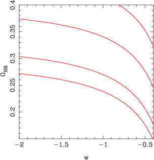
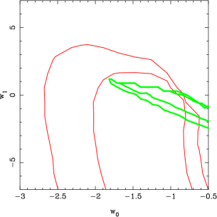
Figure 1 shows contours of equal angular diameter distance to the last scattering surface in the $\Omega_{nr}-w$ plane. We assumed a fixed value of $H_{0}$ and $\Omega_{B}$ for this plot. If the distance to the last scattering surface is the key constraint on models of dark energy then the likelihood contours should run along the contours of constant distance in this plane.

We may use the angular size of the Hubble radius at the time of decoupling as an approximate proxy for the angular size of the acoustic horizon for the purpose of this discussion. The approximate angular size $\theta$ of the Hubble radius at the time of decoupling can be written as:

$$\theta^{-1} = \frac{H_{0}/H(z)}{\int\limits_{0}^{z}{dy}/{\left(H(y)/H_{0}\right)}}$$ (6)

$$\simeq \frac{\left({\Omega_{NR}\left(1+z\right)^{3}}\right)^{-1/2}}{\int\limits_{0}^{z}{dy}/{\sqrt{\Omega_{NR}\left(1+z\right)^{3}+\varrho^{DE}(z)/\varrho^{DE}_{0}}}}$$

$$\equiv \frac{\left({\Omega_{NR}\left(1+z\right)^{3}}\right)^{-1/2}}{\int\limits_{0}^{z}{dy}/{\sqrt{\Omega_{NR}\left(1+z\right)^{3}+\Omega_{de}\left(1+z\right)^{3\left(1+w_{eff}\right)}}}}.$$

Clearly, the value of the integral will be different if we change $w_{0}$, $w^{\prime}(z=0)$ and there will also be some dependence on the parameterized form. If the location of peaks in the angular power spectrum of the CMB provide the main constraint, this can only constrain $w_{eff}$ and not all of $w_{0}$, $w^{\prime}(z=0)$ and $p$. Therefore if the present value $w_{0}<w_{eff}$ then it is essential that $w^{\prime}(z=0)>0$, and similarly if $w_{0}>w_{eff}$ then $w^{\prime}(z=0)<0$ is needed to ensure that the integrals match. Specifically, the combination of $w_{0}$, $w^{\prime}(z=0)$ and $p$ should give us $w_{eff}$ within the allowed range.

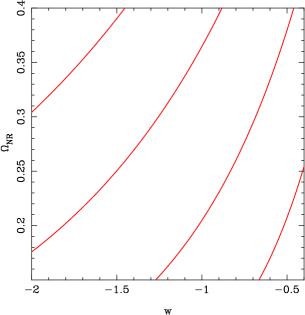
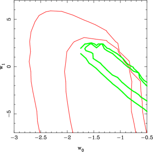
Figure 2 shows contours of constant $\theta$ in the $\Omega_{NR}-w$ plane. If the angular scale of acoustic peaks is the key constraint arising from CMB observations for models of dark energy then we should see two features in the likelihood contours:

• Likelihood contours for models with a constant equation of state parameter $w$ in the $\Omega_{NR}-w$ plane should run along contours of constant $\theta$, as shown in Figure 2.

• Likelihood contours for different models of varying dark energy should coincide in the $\Omega_{NR}-w_{eff}$ plane. These should also coincide with the contours for models with a constant $w$ in the $\Omega_{NR}-w$ plane.

The origin of the CMB constraints on dark energy therefore is not in the raw distance to the surface of last scattering but in the combination of parameters that determines the location of peaks in the angular power spectrum. It is important to note that the distance to the surface of last scattering is a derived quantity. The CMB observations constrain only one number, the effective equation of state. There is no ambiguity except for models with early dark energy (Linder & Robbers, 2008). In these models, the growth of perturbations is slower than models in which dark energy comes into play at late times (Benabed & Bernardeau, 2001; Doran & Robbers, 2006).

Figure 4: This figure shows contours of angular diameter distance (blue/dashed) and of constant angular size of the Hubble radius (red/solid) overlaid with likelihood regions allowed by WMAP5 data in the $\Omega_{NR}-w$ plane.

In our analysis, we use the angular power spectrum of the CMB temperature anisotropies (Hu & Dodelson, 2002; White & Cohn, 2002; Subramanian, 2004) as observed by WMAP (Dunkley et al., 2008; Komatsu et al., 2009) and these are compared to theoretical predictions using the likelihood program provided by the WMAP team (Dunkley et al., 2008; Komatsu et al., 2009). We vary the amplitude of the spectrum till we get the best fit with WMAP observations. The CMBFAST package (Seljak & Zaldarriaga, 1996) is used for computing the theoretical angular power spectrum for a given set of cosmological parameters. We have combined the likelihood program with the CMBFAST code and this required a few minor changes in the CMBFAST driver routine. We also made changes in the driver program to implement Monte Carlo Markov Chain for sampling the parameter space. Please see (Jassal, Bagla, & Padmanabhan, 2005a) for details of the MCMC implementation.

Although we can use other observations like abundance of rich clusters, baryonic features in the power spectrum, etc. but we find that the two observations used here are sufficient for this study (Jassal, 2009).

3 Results

In this section we will describe the results of our study. We studied models in three classes:

• Models with a constant equation of state parameter $w$. We studied models with perturbations in dark energy (Bean & Doré, 2004; Caldwell, Dave & Steinhardt, 1998; Weller & Lewis, 2003; Hannestad, 2005; Fabris, Shapiro, & Solà, 2007; Fabris & Gonçalves, 2006; Unnikrishnan, Jassal, & Seshadri, 2008; Jassal, 2009; Bartolo, Corasaniti, Liddle & Malquarti, 2004; Mota & van de Bruck, 2004; Gordon & Hu, 2004; Gordon & Wands, 2005; Nunes & Mota, 2006; Sergijenko et al., 2008; Hu, 2005; Mainini, 2009, 2008) as well as without.

• Models with a varying equation of state parameter $w$, with variation given by Eqn.3 (p=1). Perturbations in dark energy were not taken into account in this case.

• Models with a varying equation of state parameter $w$, with variation given by Eqn.3 (p=2). Perturbations in dark energy were not taken into account in this case too.

We analyse the allowed range of cosmological parameters for these cosmologies and consider the probability with which the $\Lambda$CDM model is allowed within these three classes of models. In light of the significant disagreement between the allowed range of parameters from the high redshift supernova data from the Gold+Silver set and the CMB anisotropies from WMAP observations (Jassal, Bagla, & Padmanabhan, 2005a; Nesseris & Perivolaropoulos, 2005), we also check the degree of overlap between the parameter space allowed by the supernova and the CMB observations respectively. The newly released ’Union’ dataset includes data from the Supernova Legacy Survey, the ESSENCE Survey (Wood-Vasey et al., 2007) and the extended distant supernova dataset from HST along with the older datasets (Kowalski et al., 2008). The combined data favours variation in dark energy equation of state.

Table 1: This table lists the priors used in the present work. Apart from the range of parameters listed in the table, we assumed that the universe is flat. We assumed that the primordial power spectrum had a constant index. Further, we ignored the effect of tensor perturbations. The range of values for $w_{0}$ and $w^{\prime}(z=0)$ is as given below, but with the constraint that $w(z=1000)\leq-1/3$. Any combination of $w_{0}$ and $w^{\prime}(z=0)$ that did not satisfy this constraint was not considered. Values given in parenthesis were used for analysing constraints from high redshift supernovae in §3.1.

Parameter	Lower limit	Upper limit
$\Omega_{B}$	$0.03$	$0.06$
$\Omega_{NR}$	$0.1$	$0.5(0.7)$
$h$	$0.6$	$0.8$
$\tau$	$0.0$	$0.4$
$n$	$0.86$	$1.10$
$w_{0}$	$-2.0(-4.0)$	$-0.4$
$w^{\prime}(z=0)$	$-5.0$	$5.0$

Figure 5: Marginalized likelihood contours in $\Omega_{NR}-w$ plane for different models. In the top figures the blue dashed lines correspond to 68%, 95% confidence level using the gold data. The red solid lines correspond to confidence levels in SNLS data. The black thick lines are marginalized confidence levels using WMAP5 data. The top left panel if for constant $w$ models with a homogeneous dark energy and the one on the right is when we include dark energy perturbations. The bottom left plot is for models with $p=1$ and the right plot is with $p=2$.

3.1 Cosmological Constant

We begin with a very brief review of constraints on parameters in the case where a cosmological constant is the source of accelerating expansion of the universe. We used priors given in Table 1, except that the equation of state parameter is fixed to $w=-1$. Constraints on cosmological parameters are listed in Table 2. We would like to note that our results match those obtained by other authors (Dunkley et al., 2008; Komatsu et al., 2009). Figure 3 shows contours of likelihood for some pairs of parameters as an example. We have shown contours in the $n-\Omega_{NR}h^{2}$, $n-\Omega_{B}h^{2}$, and, $n-\tau$ plane. we see that there is a strong correlation between $n-\Omega_{B}h^{2}$. These likelihood contours have also been shown as a reference for equivalent plots for models with $w\neq-1$, and help in checking the effect of the additional dark energy parameters on allowed range of other parameters.

3.2 Constant w

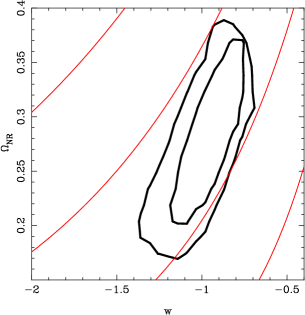
We first evaluate the nature of the CMB constraint on models of dark energy. Figure 4 shows likelihood contours from WMAP5 observations in the $\Omega_{NR}-w$ plane for constant $w$ models. We find that the orientation of these contours is roughly along contours of constant $\theta$. To illustrate this, we have overlaid contours from Figure 1 and Figure 2 in Figure 4. On the other hand there is no similarity between the likelihood and contours of distance to the last scattering surface. Thus we may conclude that the dominant constraint provided by the CMB observations arises from the location of peaks in the angular power spectrum. The reason for this is that the angular diameter distance to the last scattering surface is a derived quantity, whereas the location of peaks in the angular power spectrum of temperature anisotropies is a direct observable.

We use priors given in Table 1 for models with a constant equation of state parameter, with the obvious constraint that $w^{\prime}(z=0)=0$. For supernova observations, we used wider priors for $w$ and $\Omega_{NR}$ in order to illustrate the differences between the two data sets studied here. We begin with a brief summary of results for the Gold+Silver data set. The best fit model in this case is $w=-1.99$ and $\Omega_{NR}=0.47$. The allowed range for $w$ at $95\%$ confidence limit for large priors is $-3.73\leq w\leq-1.25$. The corresponding range for the density parameter is $0.28\leq\Omega_{NR}\leq 0.57$. With SNLS data, the best fit model is $w=-1.06$ and $\Omega_{NR}=0.29$. The allowed range for $w$ at $95\%$ confidence limit is $-2.36\leq w\leq-0.74$. The allowed range for the density parameter is $0.11\leq\Omega_{NR}\leq 0.48$. There is clearly a large shift in the allowed values of parameters.

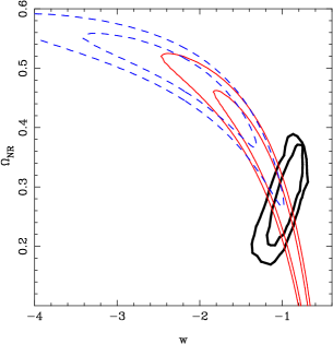
We illustrate this in Figure 5 (top-left panel) where we have plotted the regions allowed by the two data sets at $68\%$ confidence levels in the $w-\Omega_{NR}$ plane. Dashed line shows the region allowed by the Gold+Silver data set and the solid line is for the SNLS data set. We can deduce the following from this figure:

• The region allowed by these two data sets at $68\%$ confidence level has some overlap, thus we may say that the two sets are consistent with each other.

• The overlap is at $\Omega_{NR}\geq 0.36$ and is thus at margins of what is allowed by other observations.

• The $\Lambda$CDM model is ruled out at $68\%$ confidence level by the Gold+Silver data set.

• The best fit of each set is ruled out by the other data set at this confidence level. Indeed, the best fit of Gold+Silver data set is allowed by the SNLS data with a probability $\mathcal{P}=12.65\%$ while the best fit of the SNLS data set is allowed by the Gold+Silver data set with $\mathcal{P}=8.14\%$.

This point is reiterated by the likelihoods of $w$ and $\Omega_{NR}$ for these models in the same panel.

The figure shows the large overlap between the likelihood curves corresponding to SNLS data and WMAP data where the Gold+Silver data clearly favours higher values of $\Omega_{NR}$ and more negative $w$. The phantom models are still allowed but the SNLS data as well as WMAP data show a preference for models close to a cosmological constant.

For comparison, WMAP allows $-1.25\leq w\leq-0.7$ and $0.2\leq\Omega_{NR}\leq 0.38$ if dark energy is assumed to be smooth. If we allow for perturbations in dark energy then the limits on the equation of state parameters changes to $-1.25\leq w\leq-0.64$ and $0.20\leq\Omega_{NR}\leq 0.38$ as shown in the top right panel of Figure 5.

These figures allow us to conclude that:

• WMAP observations of temperature and polarization anisotropies strongly favour models around $w=-1$, i.e., the $\Lambda$CDM model. As a result, WMAP and Gold+Silver data sets have a small region of overlap as the latter does not favour models around $w=-1$. (It is this disagreement that had led us to suggest that the supernova data set could be plagued by some systematic effects (Jassal, Bagla, & Padmanabhan, 2005a), particularly as it contains supernovae from a number of different sources. In that work, we have used WMAP first year data.)

• WMAP and SNLS data sets have a region of overlap within $68\%$ confidence levels.

• There is no significant change in the likelihood contours for other cosmological parameters as we go from the cosmological constant model to dark energy with a constant equation of state parameter (not constrained to $w=-1$), or when we go from a smooth dark energy to the model where dark energy is allowed to cluster.

Thus we can say that SNLS and WMAP data are in (much) better agreement as compared to the Gold+Silver and WMAP data sets.

3.3 Varying $w(z)$

It has been claimed that observations, in particular observations of high redshift supernovae (the Gold and Gold+Silver data sets) favour evolution of dark energy (Alam et al., 2004a, b; Padmanabhan & Choudhury, 2003; Jonsson et al., 2004; Jimenez, 2003; Amendola & Quercellini, 2003; Jimenez et al., 2003; Bassett, 2004; Bassett, Corasaniti & Kunz, 2004; Corasaniti et al., 2004; Daly & Djorgovski, 2004; Gong, 2004; Choudhury & Padmanabhan, 2005; Wang, 2004; Wang et al., 2004). As such a variation is impossible if acceleration of the universe is caused by the cosmological constant, it is important to test this claim. Note that the term “Evolution of dark energy” has been used for evolution of the equation of state parameter, as well as for evolution of energy density for the dark energy component. In an earlier study using the Gold+Silver data set, we had found that supernova observations do not favour evolution of the equation of state parameter over models with a constant $w\ll-1$. But these models are favoured strongly as compared to the cosmological constant model, which was allowed with $\mathcal{P}=6.3\%$ amongst models with constant $w$. When combined with WMAP and other constraints, the allowed variation of dark energy is restricted to a narrow range and models around the Cosmological constant are favoured (Seljak et al., 2005; Jassal, Bagla, & Padmanabhan, 2005a). We should note that if we combine only the Gold+Silver (or Gold) supernova and WMAP data then results favour evolution of $\rho_{DE}$, but adding observations of galaxy clustering removes this inclination.

Figure 6: The black contours in this figure show constraints on the effective dark energy equation of state $w_{eff}$ for $p=1$ and $p=2$ from the WMAP5 data. The green lines are constraints on constant $w-\Omega_{NR}$ (without perturbations). These clearly show that the CMB data constrains effective equation of state at the last scattering surface.

Figure 7: This figure shows allowed range in variation of dark energy density as a function of redshift. The top row is for homogeneous dark energy model, the second row is for perturbed dark energy, the third row is for varying $w$ with $p=1$, and, the last row is for varying $w$ with $p=2$. The white region is the allowed range at 63% confidence level, the hatched region is the one disallowed range of dark energy density at 95% confidence level and the solid (blue) region is the one ruled out at 99% confidence level. In all the rows, the left most plot shows range allowed by SNLS data, the middle one with WMAP5 data and the right one shows the range allowed by combined data.

Table 2: This table lists the range of parameters allowed within 95% confidence limit from SNLS, WMAP1, WMAP3 and SNLS+WMAP3.

Parameter	$\Lambda$CDM	w=const.	w=const.	p=1	p=2
			with perturbations
		$-1.92$ — $-0.74$	$-1.92$—$-0.74$	$-1.89$—$-0.61$	$-1.9$—$-0.59$	SNLS
$w$		$-1.39$ — $-0.58$	$-1.63$ — $-0.66$	$-1.64$ — $-0.42$	$-1.93$ — $-0.43$	WMAP1
		$-1.25$ — $-0.7$	$-1.25$ — $-0.64$	$-1.62$ — $-0.44$	$-1.62$ — $-0.43$	WMAP5
		$-1.47$ — $-0.83$	$-1.57$ — $-0.88$	$-1.46$ — $-0.81$	$-1.74$ — $-0.77$	SNLS+WMAP1
		$-1.1$—$-0.9$	$-1.1$ — $-0.9$	$-1.3$ — $-0.8$	$-1.42$ — $-0.66$	SNLS+WMAP5
				$-4.82$—$3.3$	$-4.79$—$4.23$	SNLS
$w^{\prime}(z=0)$				$-3.09$ — $1.32$	$-2.5$ — $4.87$	WMAP1
				$-1.8$ — $1.2$	$-3.3$ — $2.7$	WMAP5
				$-0.99$ — $1.04$	$-2.22$ — $4.79$	SNLS+WMAP1
				$-1.25$ — $0.91$	$-2.6$ — $2.7$	SNLS+WMAP5
	$0.22$—$0.31$	$0.11$—$0.47$	$0.11$—$0.47$	$0.11$—$0.48$	$0.11$—$0.48$	SNLS
$\Omega_{NR}$	$0.20$ — $0.45$	$0.16$ — $0.43$	$0.20$ — $0.47$	$0.17$ — $0.45$	$0.18$ — $0.44$	WMAP1
	$0.19$ — $0.33$	$0.19$ — $0.38$	$0.19$ — $0.39$	$0.19$ — $0.39$	$0.19$ — $0.38$	WMAP3
	$0.21$ — $0.34$	$0.2$ — $0.38$	$0.2$ — $0.38$	$0.2$ — $0.38$	$0.20$ — $0.38$	WMAP5
	$0.22$—$0.31$	$0.15$—$0.36$	$0.18$ — $0.41$	$0.16$—$0.38$	$0.19$—$0.39$	SNLS+WMAP1
	$0.22$ — $0.3$	$0.22$ — $0.3$	$0.22$ — $0.3$	$0.22$ — $0.33$	$0.21$ — $0.32$	SNLS+WMAP5
$h$	$0.61$ — $0.79$	$0.61$ — $0.78$	$0.6$ — $0.79$	$0.6$ — $0.78$	$0.61$ — $0.78$	WMAP1
	$0.66$ — $0.77$	$0.60$ — $0.78$	$0.60$ — $0.78$	$0.61$ — $0.79$	$0.61$ — $0.78$	WMAP5
	$0.69$—$0.77$	$0.68$—$0.78$	$0.68$—$0.79$	$0.67$—$0.77$	$0.65$—$0.78$	SNLS+WMAP1
	$0.68$—$0.74$	$0.68$—$0.74$	$0.68$—$0.74$	$0.66$ — $0.76$	$0.65$ — $0.76$	SNLS+WMAP5
$\Omega_{B}h^{2}$	$0.02$ — $0.027$	$0.021$ — $0.028$	$0.02$ — $0.027$	$0.02$ — $0.027$	$0.02$ — $0.027$	WMAP1
	$0.021$ — $0.024$	$0.021$ — $0.023$	$0.02$ — $0.024$	$0.021$ — $0.0235$	$0.022$ — $0.024$	WMAP5
	$0.02$ — $0.027$	$0.021$—$0.027$	$0.021$—$0.027$	$0.021$—$0.027$	$0.021$—$0.028$	SNLS+WMAP1
	$0.021$ — $0.023$	$0.021$—$0.024$	$0.021$—$0.024$	$0.021$ — $0.023$	$0.021$ — $0.024$	SNLS+WMAP5
$n$	$0.93$ — $1.08$	$0.93$ — $1.1$	$0.93$ — $1.09$	$0.93$ — $1.1$	$0.93$ — $1.098$	WMAP1
	$0.94$ — $0.99$	$0.93$ — $0.99$	$0.93$ — $0.99$	$0.93$ — $0.99$	$0.93$ — $0.99$	WMAP5
	$0.93$ — $1.09$	$0.94$—$1.08$	$0.94$—$1.09$	$0.93$ — $1.09$	$0.93$ — $1.097$	SNLS+WMAP1
	$0.94$ — $0.99$	$0.94$—$0.99$	$0.93$—$0.99$	$0.93$ — $0.99$	$0.94$ — $0.99$	SNLS+WMAP5
$\tau$	$0.002$ — $0.33$	$0.011$ — $0.39$	$0.007$ — $0.35$	$0.13$ — $0.4$	$0.016$ — $0.39$	WMAP1
	$0.054$ — $0.12$	$0.05$ — $0.12$	$0.055$ — $0.12$	$0.054$ — $0.12$	$0.054$ — $0.12$	WMAP5
	$0.004$ — $0.33$	$0.008$—$0.34$	$0.045$—$0.37$	$0.013$ — $0.38$	$0.017$ — $0.396$	SNLS+WMAP1
	$0.054$ — $0.12$	$0.053$—$0.12$	$0.055$—$0.13$	$0.52$ — $0.12$	$0.05$ — $0.125$	SNLS+WMAP5

We studied constraints on models of varying dark energy with the SNLS and WMAP5 data and the results are summarised in table 2, which gives the ranges of parameters allowed at $95\%$ confidence level. The supernova data constrains $w_{0}$ but does not effectively constrain $w_{1}$. On the other hand, CMB data constrains an effective equation of state and hence indirectly provides constraints on $w^{\prime}(z=0)$. This is evident from lower panels of Figure 5, where we have plotted confidence contours in $\Omega_{NR}-w$ plane. The CMB contours are significantly narrower than those given by the Supernova data. We do not find any significant changes in the likelihood contours for other parameters such as $n$, $\Omega_{NR}h^{2}$, $\Omega_{B}h^{2}$ and $\tau$. For instance the range of $\Omega_{NR}h^{2}$ is given by $0.21-0.33$ is valid for all the models considered here. This is illustrated in Table 2.

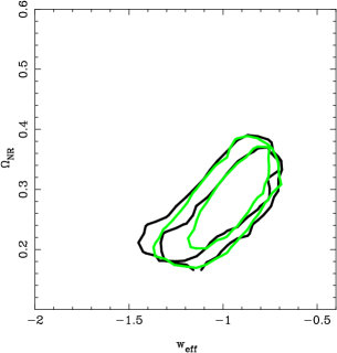
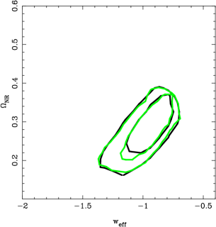
Given that CMB observations constrain only one number, we expect that the constraint on models with varying $w(z)$ should constrain only $w_{eff}$ as defined in Eqn.(6). We confirm this by plotting likelihood contours for models with varying $w(z)$ on the $\Omega_{NR}-w_{eff}$ plane. We also plot contours for constant $w$ models on the same plane for reference. Figure 6 shows these contours for the models with $p=1$ and $p=2$. We find very strong coincidence in the contours for models with variable $w(z)$ when plotted with $w_{eff}$ with the contours for models with constant $w$ thereby confirming our conjecture. This also provides an easy approach to constraining models with variable $w(z)$ without detailed calculations, all that one needs is to check whether $w_{eff}$ is in the range allowed by CMB observations for $w$ in the constant $w$ model.

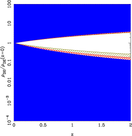
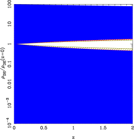
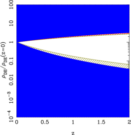
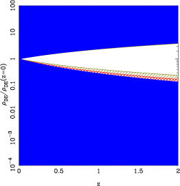
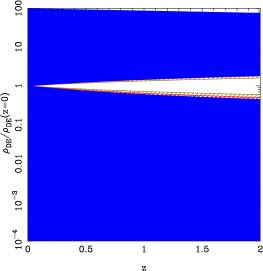
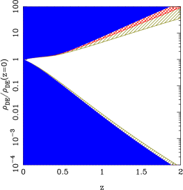
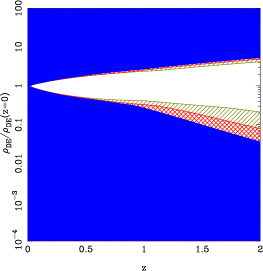
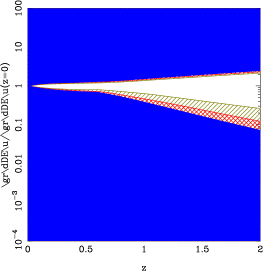
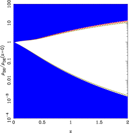
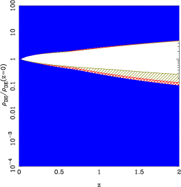
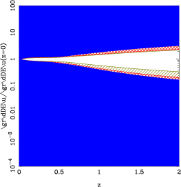
We return to the issue of variation of dark energy density allowed by observations. A pictorial representation of results is given in Figure 7, where we have plotted $\rho_{DE}(z)/\rho_{DE}(z=0)$ as a function of redshift. Different panels show the evolution of this quantity as allowed by the SNLS data set, WMAP5 observations of temperature and polarization anisotropies in the CMB and combined constraints from WMAP5+SNLS. These are plotted for constant $w$ (with and without dark energy perturbations), and for variable $w$ with $p=1$ and $p=2$. Dark energy was assumed to be homogeneous in all cases except for the second row that corresponds to constant $w$ models with perturbations in dark energy. We can conclude that:

• Supernova observations are a tight constraint for models with constant $w$, but these are not as strong as CMB constraints.

• SNLS+WMAP5 data offers tighter constraints than either data set and the cosmological constant is allowed with a high probability. This follows from the complementary nature of the two constraints as seen from the orientation of the likelihood contours (e.g., see Figure 5).

• Supernova observations do not constrain evolution of dark energy density in models with a variable $w$. Very large variation in dark energy density is allowed by these observations.

• WMAP5 observations are, in contrast, a much tighter constraint and do not allow significant variation in dark energy. Indeed, the variation in dark energy density allowed by WMAP5 observations for models with variable $w$ is not significantly larger than that allowed for constant $w$ models.

• We demonstrate that the constraints on dark energy parameters for varying $w$ models are the same as the constraints on constant $w$ models if we consider $w_{eff}$ for varying dark energy models.

• SNLS+WMAP constraints are essentially dominated by the WMAP data and follow the same pattern. SNLS observations add to the overall constraint by limiting the range of values allowed for $w_{0}$.

We would like to add a note of caution that the analysis for varying $w$ models does not take perturbations in dark energy into account. However, these are more important for $w\gg-1$ or models with rapidly varying $w$ (Bean & Doré, 2004; Caldwell, Dave & Steinhardt, 1998; Weller & Lewis, 2003; Hannestad, 2005) and such models are not allowed by observational constraints.

4 Discussion

In this work we studied the SNLS data set and compared the constraints obtained with constraints from WMAP five year data on temperature anisotropies in the CMB. We find that the parameter values favoured by the two data sets have significant overlap and the two sets can be combined to put tight constraints on models of dark energy. In an earlier work we had noted that the Gold+Silver data set does not agree with WMAP observations in that these favour distinct parts of the parameter space (Jassal, Bagla, & Padmanabhan, 2005a). Constraints from WMAP and structure formation favour similar models, but ones distinct from those favoured by Gold+Silver supernova observations. This indicates some degree of inconsistency between the supernova and other observations and it led us to suggest that the Gold+Silver data set may be affected by as yet unknown systematic errors (Jassal, Bagla, & Padmanabhan, 2005a). One reason for doubting the supernova data is the heterogeneity of sources from which the particular data set was collected (Riess et al., 2004). SNLS (Astier et al., 2005) is a homogeneous data set and should not suffer from such problems and indeed we find that there is no inconsistency between SNLS and WMAP observations.

This highlights the usefulness of CMB observations for constraining models of dark energy (Eisenstein & White, 2004; Jassal, Bagla & Padmanabhan, 2005). We believe that CMB observations should be used for testing any model of dark energy as supernova observations do not constrain models with varying $w$ effectively . Thus one should use CMB observations as well and not rely only on supernova observations for constraining such models.

We would like to add a note of caution against combining the SNLS data with other data sets of high redshift supernovae in light of the very different nature of these data sets. Indeed, one should use homogeneous data sets like the SNLS in isolation to avoid the problems mentioned above.

In terms of models, we find that the cosmological constant is favoured by individual observations (SNLS and WMAP) as well as in the combined data set with very high probability. Table 2 gives allowed values of all cosmological parameters at $95\%$ confidence level by SNLS, WMAP as well as the combined data set. For the cases where a similar analysis has been done by others, our results are consistent with other findings (Bridle et al., 2003; Spergel et al., 2003; Maccio et al., 2003; Linder & Jenkins, 2003; Pogosyan, Bond & Contaldi, 2003; Tegmark et al., 2004; Wang & Tegmark, 2004; Giovi, Baccigalupi & Perrotta, 2004; Hannestad, 2004; Huterer & Cooray, 2004; Lee, 2005; Lee & Ng, 2003; Lee, Lee & Ng, 2003; Mainini, Colombo & Bonometto, 2005; Rapetti, Allen & Weller, 2004; Pogosyan, 2004; Nesseris & Perivolaropoulos, 2005; Seljak et al., 2005; Shen, Wang, Abdalla & Su, 2005; Feng, Wang & Zhang, 2005; Xia et al., 2006a, b; Amendola, Campos, & Rosenfeld, 2007; Calvo & Maroto, 2006; Carneiro et al., 2006; Dantas et al., 2007; Elizalde et al., 2008; Mota, Kristiansen, Koivisto & Groeneboom, 2007).

We have discussed the origin of the constraint on dark energy models from CMB observations at length. We may conclude from the analysis presented here that:

• Location of acoustic peaks in the angular power spectrum of CMB anisotropies is the main source of constraints.

• CMB observations only constrain $w_{eff}$, an effective value of the equation of state parameter defined in Eqn.(6). This can be used to translate constraints on models with constant $w$ to models where dark energy properties vary with time.

• We have discussed models with $\Omega_{0}=1$ in this paper. In case this constraint is relaxed then the well known degeneracy between $w$ and $\Omega_{0}$ loosens the constraints. However, it is well known that the SN and CMB data are complementary and can be combined to provide fairly tight constraints even in this case (Perlmutter, Turner & White, 1999; Huterer & Turner, 2001). We do not expect variations in curvature to modify our conclusions about $w_{eff}$ being the only dark energy related quantity constrained by CMB observations.

• Integrate Sachs-Wolfe (ISW) effect due to perturbations in dark energy can, in principle, lead to variations in the CMBR angular power slectrum at small $l$. Our analysis of models with variable $w$ without perturbations does not take this into account. Various analyses have shown that ISW does not contribute significantly to constraining cosmological parameters from CMB data (see for example, (Xia et al., 2009)). The main reason for this is that ISW affects power at small $l$, and due to large cosmic variance these modes do not contribute much to the overall likelihood.

References

- Andrianov, Cannata & Kamenshchik (2005) Andrianov A. A., Cannata F., Kamenshchik A. Y., 2005, Phys. Rev. D 72, 043531
- Aguirregabiria & Lazkoz (2004) Aguirregabiria J. M., Lazkoz R., hep-th/0402190
- Alam et al. (2004a) Alam U., Sahni V., Starobinsky A. A., 2004, JCAP, 0406, 008
- Alam et al. (2004b) Alam U., Saini T.D., Sahni V., Starobinsky A. A., 2004, Mon. Not. Roy. Astron. Soc., 354, 275
- Alcaniz (2006) Alcaniz, J. S., 2006, Braz. J. Phys., 36, 1109
- Amendola & Quercellini (2003) Amendola L., Quercellini C., 2003, Phys. Rev. D 68, 023514
- Amendola, Campos, & Rosenfeld (2007) Amendola L., Campos G. C., Rosenfeld R., 2007, PhRvD, 75, 083506
- Apostolopoulos & Tetradis (2006) Apostolopoulos P. S., Tetradis N., 2006, PhRvD, 74, 064021
- Armendariz-Picon, Mukhanov, & Steinhardt (2001) Armendariz-Picon C., Mukhanov V., Steinhardt P. J., 2001, PhRvD, 63, 103510
- Arianto et al. (2007) Arianto, Zen F. P., Gunara B. E., Triyanta, Supardi, 2007, JHEP, 9, 48
- Astier et al. (2005) Astier P. et al. 2005, astro-ph/0510447
- Bagla, Padmanabhan & Narlikar (1996) Bagla J. S., Padmanabhan T., Narlikar J. V., 1996, Comments on Astrophysics 18, 275; astro-ph/9511102
- Bartolo, Corasaniti, Liddle & Malquarti (2004) Bartolo N., Corasaniti P.-S., Liddle A. R., Malquarti M., 2004, PhRvD, 70, 043532
- Jassal (2009) Jassal H. K., in preparation
- Bagla, Jassal & Padmanabhan (2003) Bagla J. S., Jassal H. K., Padmanabhan T., 2003, Phys. Rev. D 67, 063504; astro-ph/0212198
- Barris et al. (2004) Barris B. J., et al., 2004, ApJ, 602, 571
- Bassett (2004) Bassett B. A., astro-ph/0407201
- Bassett, Corasaniti & Kunz (2004) Bassett B. A., Corasaniti P. S., Kunz M., 2004, Astrophys. J., 617, L1
- Bean & Doré (2004) Bean R., Doré O., 2004, Phys. Rev. D 69, 083503
- Benabed & Bernardeau (2001) Benabed K., Bernardeau F., 2001, Phys. Rev. D 64, 083501
- Bento, Bertolami & Sen (2002) Bento M. C., Bertolami O., Sen A. A., 2002, Phys. Rev. D 66, 043507
- Bludman & Roos (2002) Bludman S. A., Roos M., 2002, Phys. Rev. D 65, 043503
- Bridle et al. (2003) Bridle S. L., Lahav O., Ostriker J. P., Steinhardt P. J., 2003, Sci, 299, 1532
- Briscese et al. (2007) Briscese F., Elizalde E., Nojiri S., Odintsov S. D., 2007, PhLB, 646, 105
- Bronnikov, Fabris, & Gonçalves (2007) Bronnikov K. A., Fabris J. C., Gonçalves S. V. B., 2007, JPhA, 40, 6835
- Bronnikov & Starobinsky (2007) Bronnikov K. A., Starobinsky A. A., 2007, JETPL, 85, 1
- Burgess (2003) Burgess C. P., 2003, Int. J. Mod. Phys. D 12, 1737
- Calvo & Maroto (2006) Calvo G. B., Maroto A. L., 2006, PhRvD, 74, 083519
- Carneiro et al. (2006) Carneiro S., Pigozzo C., Borges H. A., Alcaniz J. S., 2006, PhRvD, 74, 023532
- Carroll, Press, & Turner (1992) Carroll S. M., Press W. H., Turner E. L., 1992, ARA&A, 30, 499
- Carroll, Hoffman & Trodden (2003) Carroll S. M., Hoffman M., Trodden M., 2003, Phys. Rev. D 68, 023509
- Caldwell (2002) Caldwell R. R., 2002, Phys. Lett. B 545, 23
- Caldwell, Dave & Steinhardt (1998) Caldwell R. R., Dave R., Steinhardt P. J., 1998, Phys. Rev. Lett. 80, 1582
- Chiba (2002) Chiba T., 2002, Phys. Rev. D 66, 063514
- Chimento & Feinstein (2004) Chimento L. P., Feinstein A., 2004, Mod. Phys. Lett. A 19, 761
- Choudhury & Padmanabhan (2005) Choudhury T. R., Padmanabhan T.,Astron.Astrophys., 429: 807, (2005) [astro-ph/0311622]
- Choudhury et al. (2002) Choudhury D., Ghoshal D., Jatkar D. P., Panda S., 2002, Phys. Lett. B 544, 231
- Clarkson, Cortês, & Bassett (2007) Clarkson C., Cortês M., Bassett B., 2007, JCAP, 8, 11
- Cline, Jeon & Moore (2003) Cline J. M., Jeon S. Y., Moore G. D., 2004, Phys. Rev. D 70, 043543
- Cognola, Elizalde, Nojiri, Odinstov & Zerbini (2006) Cognola G., Elizalde E., Nojiri S., Odinstov S. D., Zerbini S., hep-th/0601008
- Copeland, Sami & Tsujikawa (2006) Copeland, E. J. and Sami, M. and Tsujikawa, S., 2006, Int. J. Mod. Phys. D 15, 1753
- Corasaniti et al. (2004) Corasaniti P. S., Kunz M., Parkinson D., Copeland E. J., Bassett B. A., astro-ph/0406018
- Dabrowski, Stachowiak & Szydlowski (2003) Dabrowski M. P., Stachowiak T., Szydlowski M., 2003, Phys. Rev. D 68, 103519
- Daly & Djorgovski (2004) Daly R. A., Djorgovski S. G., astro-ph/0405063
- Dantas et al. (2007) Dantas M. A., Alcaniz J. S., Jain D., Dev A., 2007, A&A, 467, 421
- Dunkley et al. (2008) Dunkley J. et al., Astrophys. J. Suppl. 180, 306
- Das, Banerjee & Dadhich (2005) Das S.,Banerjee N., Dadhich N., astro-ph/0505096
- Dev, Jain & Alcaniz (2003) Dev A., Jain D., Alcaniz J. S., 2003, Phys. Rv. D 67, 023515
- Doran & Robbers (2006) Doran M., Robbers G., 2006, JCAP, 6, 26
- Efstathiou, Sutherland & Maddox (1990) Efstathiou G., Sutherland W. J., Maddox S. J., 1990, Nature 348, 705
- Eisenstein & White (2004) Eisenstein D. J., White M., 2004, PhRvD, 70, 103523
- Elizalde, Nojiri, & Odintsov (2004) Elizalde E., Nojiri S., Odintsov S. D., 2004, PhRvD, 70, 043539
- Elizalde et al. (2008) Elizalde E., Nojiri S., Odintsov S. D., Sáez-Gómez D., Faraoni V., 2008, arXiv, 803, arXiv:0803.1311
- Ellis (2003) Ellis J. R., 2003, Phil. Trans. Roy. Soc. Lond. A 361, 2607
- Fabris, Shapiro, & Solà (2007) Fabris J. C., Shapiro I. L., Solà J., 2007, JCAP, 2, 16
- Fabris & Gonçalves (2006) Fabris J. C., Gonçalves S. V. B., 2006, PhRvD, 74, 027301
- Feng, Wang & Zhang (2005) Feng B., Wang X., Zhang X., 2005, Phys. Lett. B 607, 35
- Frampton (2003) Frampton P. H., hep-th/0302007
- Frolov, Kofman & Starobinsky (2002) Frolov A. V., Kofman L., Starobinsky A. A., 2002, Phys. Lett. B 545, 8
- Garnavich et al. (1998) Garnavich P. M., et al., 1998, ApJ, 509, 74
- Gibbons (2002) Gibbons G. W., 2002, Phys. Lett. B 537, 1
- Gibbons (2003) Gibbons G. W., 2003, Class. Quant. Grav. 20, S321
- Gibbons (2003) Gibbons G. W., hep-th/0302199
- Giovi, Baccigalupi & Perrotta (2004) Giovi F., Baccigalupi C., Perrotta F., astro-ph/0411702
- Gong (2004) Gong Y. G., astro-ph/0401207
- Gonzalez-Diaz (2002) Gonzalez-Diaz P. F., 2002, Phys. Rev. D 62, 023513
- Gonzalez-Diaz (2000) Gonzalez-Diaz P. F., 2000, Phys. Lett. B 481, 353
- Gonzalez-Diaz (2003) Gonzalez-Diaz P. F., 2003, Phys. Rev. D 68, 021303
- Gorini et al. (2004) Gorini V., Kamenshchik A. Y., Moschella U., Pasquier V., 2004, PhRvD, 69, 123512
- Gordon & Hu (2004) Gordon C., Hu W., 2004, PhRvD, 70, 083003
- Gordon & Wands (2005) Gordon C., Wands D., 2005, PhRvD, 71, 123505
- Gorini et al. (2001) Gorini V., Kamenshchik A. Y., Moschella U., Pasquier V., 2001, Phys. lett. B 511, 265
- Hannestad (2004) Hannestad S., 2004, JCAP, 0409, 001
- Hannestad (2005) Hannestad S., 2005, Phys. Rev. D 71, 103519
- Hannestad & Mortsell (2004) Hannestad S., Mortsell E., 2004 JCAP, 0409, 001
- Hao & Li (2003) Hao J. g. Li X. z., 2003, Phys. Rev. D 67, 107303
- Holman & Naidu (2004) Holman R. and Naidu S. 2004, astro-ph/0408102
- Hu (2005) Hu W., 2005, PhRvD, 71, 047301
- Hu & Dodelson (2002) Hu W., Dodelson S., 2002, ARA&A, 40, 171
- Huterer & Turner (2001) Huterer D., Turner M. S., 2001, PhRvD, 64, 123527
- Huterer & Cooray (2004) Huterer D., Cooray A., astro-ph/0404062
- Jain & Ralston (2005) Jain P. and Ralston J. P. 2005, ApJ In Press, astro-ph/0506478
- Jassal (2004) Jassal H. K., 2004, Pramana 62, 757
- Jassal (2003) Jassal H. K., hep-th/0312253
- Jassal, Bagla & Padmanabhan (2005) Jassal H. K., Bagla J. S., Padmanabhan T., 2005, Mon. Not. Roy. Astron. Soc. 356, L11-L16; astro-ph/0404378
- Jassal, Bagla, & Padmanabhan (2005a) Jassal H. K., Bagla J. S., Padmanabhan T., 2005, PhRvD, 72, 103503; astro-ph/0506748
- Jassal (2009) Jassal H. K., arXiv:0903.5370
- Jimenez (2003) Jimenez R., 2003, New Astron. Rev. 47, 761
- Jimenez et al. (2003) Jimenez R., Verde L., Treu T., Stern D., 2003, Astrophys. J. 593, 622
- Jonsson et al. (2004) Jonsson J., Goobar A., Amanullah R., Bergstrom L., astro-ph/0404468
- Komatsu et al. (2009) Komatsu E., et al., 2009, ApJS, 180, 330
- Kowalski et al. (2008) Kowalski M., et al., 2008, ApJ, 686, 749
- Kim, Kim & Kim (2003) Kim C. j., Kim H. B., Kim Y. b., 2003, Phys. Lett. B 552, 111
- Lazkoz, Neseseris & Perivolaropoulos (2005) Lazkoz R., Nesseris S., Perivolaropoulos L., astro-ph/0503230
- Lee (2005) Lee S., astro-ph/0504650
- Lee & Ng (2003) Lee W., Ng K., 2003, Phys. Rev. D 67 107302
- Lee, Lee & Ng (2003) Lee D., Lee W., Ng K., astro-ph/0309316
- Li (2004) Li M., 2004, Phys. Lett. B603
- Li et al. (2008) Li H., Xia J., Zhao G., Fan Z., Zhang X., 2008, ApJL, L1
- Linder & Jenkins (2003) Linder E. V., Jenkins A., 2003, Mon. Not. Roy. Astron. Soc. 346, 573
- Linder & Robbers (2008) Linder E. V., Robbers G., 2008, JCAP, 0806, 004
- de la Macorra & Piccinelli (2000) de la Macorra A., Piccinelli G., 2000,Phys. Rev. D 61, 123503
- Maccio et al. (2003) Maccio A. V., Bonometto S. A., Mainini R., Klypin A., astro-ph/0309439
- Mainini, Colombo & Bonometto (2005) Mainini R., Colombo P.L., Bonometto S. A., astro-ph/0503036
- Mainini (2009) Mainini R., 2009, JCAP 0904, 017
- Mainini (2008) Mainini R., 2008, JCAP 0807, 003
- Malquarti et al. (2003) Malquarti M., Copeland E. J., Liddle A. R., Trodden M., 2003, Phys. Rev. D 67, 123503
- Melchiorri et al. (2000) Melchiorri A. et al. [Boomerang Collaboration], 2000, Astrophys. J. 536, L63
- Milton (2003) Milton K. A., 2003, Grav. Cosmol. 9, 66
- Mota & van de Bruck (2004) Mota D. F., van de Bruck C., 2004, A&A, 421, 71
- Mota, Kristiansen, Koivisto & Groeneboom (2007) Mota D. F., Kristiansen J. R., Koivisto T., Groeneboom N. E., 2007, Mon. Not. R. Astron. Soc. 382, 793
- Nesseris & Perivolaropoulos (2005) Nesseris S., Perivolaropoulos L., 2005, Phys. Rev. D 72, 123519
- Nojiri & Odinstov (2003) Nojiri S., Odintsov S. D., 2003, Phys. Lett. B 562, 147
- Nojiri, Odintsov, & Tsujikawa (2005) Nojiri S., Odintsov S. D., Tsujikawa S., 2005, PhRvD, 71, 063004
- Nunes & Mota (2006) Nunes N. J., Mota D. F., 2006, MNRAS, 368, 751
- Onemli & Woodard (2002) Onemli V. K ., Woodard R. P., 2002, Class. Quant. Grav. 19, 4607
- Onemli & Woodard (2004) Onemli V. K., Woodard R. P., 2004, Phys. Rev. D 70, 107301
- Ostriker & Steinhardt (1995) Ostriker J. P., Steinhardt P. J., 1995, Nature 377, 600
- Padmanabhan (2002) Padmanabhan T., 2002, PhRvD, 66, 021301; hep-th/0204150
- Padmanabhan (2002) Padmanabhan T., 2002, Class. Quant. Grav. 19, 5387; gr-qc/0204019
- Padmanabhan (2003) Padmanabhan T., 2003, Phys. Rept. 380, 235; hep-th/0212290
- Padmanabhan & Choudhury (2003) Padmanabhan T., Choudhury T. R., 2003, Mon. Not. Roy. Astron. Soc. 344, 823; astro-ph/0212573
- Padmanabhan (2005a) Padmanabhan T., 2005, Curr. Sci. 88, 1057; astro-ph/0411044
- Padmanabhan (2005b) Padmanabhan T., Understanding Our Universe: Current Status and Open Issues; gr-qc/0503107
- Padmanabhan (2005c) Padmanabhan T., 2005, Phys. Rept. 49, 406; gr-qc/0311036
- Padmanabhan (2005d) Padmanabhan T., astro-ph/0510492
- Padmanabhan (2005e) Padmanabhan T., gr-qc/0510015
- Peebles & Ratra (2003) Peebles P. J. E., Ratra B., 2003, Rev. Mod. Phys. 75, 559
- Peiris and Spergel (2000) Peiris H. V. and Spergel D. N. 2000, ApJ 540, 605
- Perivolaropoulos (2005) Perivolaropoulos L., astro-ph/0601014
- Percival et al. (2007) Percival W. J., et al., 2007, ApJ, 657, 645
- Perlmutter et al. (1999) Perlmutter S., et al., 1999, ApJ, 517, 565
- Perlmutter, Turner & White (1999) Perlmutter S., Turner M. S., White M., 1999, Phys. Rev. Lett. 83, 670
- Perlmutter and Schmidt (2003) Perlmutter S. and Schmidt B. P. 2003, astro-ph/0303428
- Pogosyan (2004) Pogosyan L., astro-ph/0409059
- Pogosyan, Bond & Contaldi (2003) Pogosyan D., Bond J. R., Contaldi C. R., astro-ph/0301310
- Polarski & Ranquet (2005) Polarski D., Ranquet A., 2005, Phys. Lett. B 627, 1
- Rapetti, Allen & Weller (2004) Rapetti D., Allen S. W., Weller J., astro-ph/0409574
- Ren & Meng (2005) Ren J., Meng X., astro-ph/0511163
- de Ritis & Marino (2001) de Ritis R., Marino A. A., 2001, Phys. Rev. D 64, 083509
- Riess et al. (1998) Riess A. G., et al., 1998, AJ, 116, 1009
- Riess et al. (2004) Riess A. G., et al., 2004, ApJ, 607, 665
- Rubano & Scudellaro (2002) Rubano C., Scudellaro P., 2002, Gen. Rel. Grav. 34, 307
- Sahni & Starobinsky (2000) Sahni V., Starobinsky A. A., 2000, Int. J. Mod. Phys. D 9, 373
- Sahni & Shtanov (2003) Sahni V., Shtanov Y., 2003, JCAP 0311, 014
- Sahni, Shafieloo & Starobinsky (2008) Sahni V., Shafieloo A., Starobinsky A., 2008, Phys. Rev. D78, 103502
- Scherrer (2004) Scherrer R. J., astro-ph/0402316
- Seljak & Zaldarriaga (1996) Seljak U. and Zaldarriaga M. 1996, ApJ 469, 437.
- Seljak et al. (2005) Seljak U., et al., 2005, PhRvD, 71, 103515
- Sen (2003) Sen A., hep-th/0312153
- Sen & Seshadri (2003) Sen S., Seshadri T. R., 2003, Int. J. Mod. Phys. D 12, 445
- Sen & Scherrer (2005) Sen A. A., Scherrer R. J., 2005, Phys. Rev. D 72, 063511
- Sergijenko et al. (2008) Sergijenko O., Kulinich Y., Novosyadlyj B., Pelykh V., 2008, arXiv, arXiv:0809.3349
- Shashikant (2005) Gupta S., Saini T. D., Laskar T., 2007, astro-ph/0701683
- Shen, Wang, Abdalla & Su (2005) Shen J., Wang B., Abdalla E., Su R., 2005, Phys. Lett. B 609, 200
- Shiu & Wasserman (2002) Shiu G., Wasserman I., 2002, Phys. Lett. B 541, 6
- Singh, Sami & Dadhich (2003) Singh P., Sami M., Dadhich N., 2003, Phys. Rev. D 68, 023522
- Sola & Stefancic (2005) Sola J., Stefancic H., astro-ph/0507110
- Spergel et al. (2003) Spergel D. N. et al., 2003, ApJS 148, 175
- Steinhardt (2003) Steinhardt P. J., Royal Society of London Philosophical Transactions Series A, 361, 2497
- Subramanian (2004) Subramanian K., astro-ph/0411049
- Tegmark et al. (2004) Tegmark M., et al., 2004, ApJ, 606, 702
- Tonry et al. (2003) Tonry J. L. et al., 2003, ApJ 594, 1
- Unnikrishnan, Jassal, & Seshadri (2008) Unnikrishnan S., Jassal H. K., Seshadri T. R., 2008, arXiv:0801.2017
- Urena-Lopez & Matos (2000) Urena-Lopez L. A., Matos T., 2000, Phys. Rev. D 62, 081302
- Uzawa & Soda (2001) Uzawa K., Soda J., 2001, Mod. Phys. Lett. A 16, 1089
- Virey et al. (2005) Virey J.-M., Taxil P., Tilquin A., Ealet A., Tao C., Fouchez D., 2005, PhRvD, 72, 061302
- Wang (2004) Wang Y., astro-ph/0404484
- Wang & Tegmark (2004) Wang Y., Tegmark M., 2004, Phys.Rev.Lett.92, 241302
- Wang et al. (2004) Wang Y. et al., astro-ph/0402080
- Weinberg (1989) Weinberg S. 1989, Rev.Mod.Phys. 61, 1
- Weller & Lewis (2003) Weller J., Lewis A. M., Mon. Not. R. Astron. Soc., 2003, 346, 987
- White & Cohn (2002) White M., Cohn J. D., astro-ph/0203120
- Wood-Vasey et al. (2007) Wood-Vasey W. M., et al., 2007, ApJ, 666, 694
- Xia et al. (2006a) Xia J., Zhao G., Feng B., Li H., Zhang X., 2006, Phys. Rev. D 73, 063521
- Xia et al. (2006b) Xia J., Zhao G., Li H., Feng B., Zhang X., astro-ph/0605366
- Xia et al. (2008) Xia J., Li H., Zhao G., Zhang X., 2008, Phys. Rev. D78, 0835254
- Xia et al. (2009) Xia J.-Q., Viel M., Baccigalupi C., Matarrese S., 2009, JCAP, 9, 3