Large-Scale Bulk Motions Complicate the Hubble Diagram

Abstract

We investigate the extent to which correlated distortions of the luminosity distance-redshift relation due to large-scale bulk flows limit the precision with which cosmological parameters can be measured. In particular, peculiar velocities of type 1a supernovae at low redshifts, $z<0.2$, may prevent a sufficient calibration of the Hubble diagram necessary to measure the dark energy equation of state to better than 10%, and diminish the resolution of the equation of state time-derivative projected for planned surveys. We consider similar distortions of the angular-diameter distance, as well as the Hubble constant. We show that the measurement of correlations in the large-scale bulk flow at low redshifts using these distance indicators may be possible with a cumulative signal-to-noise ratio of order 7 in a survey of 300 type 1a supernovae spread over 20,000 square degrees.

Introduction.—The challenge to discover the nature of dark energy is pushing all methods and measures of cosmology to their limits. The luminosity distances to type 1a supernovae (SNe) which first revealed the cosmic acceleration Schmidt:1998ys ; Riess:1998cb ; Perlmutter:1998np , are now being pursued to obtain tighter constraints on cosmological model parameters Tonry:2003zg ; Knop:2003iy ; Riess:2004nr ; Astier:2005qq . Observational programs, such as the Supernova Legacy Survey (http://www.cfht.hawaii.edu/SNLS/), the Supernova Factory (http://snfactory.lbl.gov), Essence (http://www.ctio.noao.edu/ wsne/), the Carnegie Supernova Project (http://csp1.lco.cl/$\sim$cspuser1/CSP.html), in addition to ongoing efforts by existing groups, are currently underway, hoping to achieve $\sim 10\%$ constraints on the dark energy equation of state parameter. In order to decisively advance our understanding, and test for a possible time-evolution of the dark energy, a dedicated space-based mission is planned as part of the NASA/DOE Joint Dark Energy Mission (JDEM).

The luminosity distance-redshift relation, however, has a basic limitation as a tool for cosmology in an inhomogeneous universe. Large scale structures distort the distances and redshifts. It is well known that peculiar velocities of SNe induced by the internal properties of host galaxies and clusters contribute a random component to distance estimates which can be reduced by averaging over many SNe. Furthermore, gravitational lensing of SN light reduces the accuracy with which the true luminosity distance can be determined for an individual SN Gunn:1967 ; Frieman ; HWa ; HWb , thereby complicating an easy interpretation of the Hubble diagram. The effect comes from the slight modification of the observed SN flux due to lensing by the intervening large-scale structure Wang:2002qc ; Holz:2004xx ; Wang:2004ax ; Gunnarsson:2005qu and correlates distance errors of SNe spread over the sky at a few degrees or less, due to survey geometries in the form of “pencil beams” or long, but narrow strips Cooray:05 . Our primary concern in this paper is large-scale bulk flows Strauss:1995fz , peculiar motions that are coherent on scales above $\sim 60$ Mpc, which correlate individual SN distance estimates spread over ten or more degrees angular scale. In this case the effect comes from the slight Doppler shifting of both the source and observer, affecting both the inferred redshift and the flux, resulting in a non-linear correction to the luminosity distance. This correlated noise cannot be reduced simply by increasing the sample size and is expected to affect the error budget from low to intermediate redshifts ($z<0.2$). Because the Hubble diagram at these low redshifts must be pinned down accurately in order that we may hope to find a possible time variation in the dark energy equation of state Kim:2003mq ; Huterer:2004rf , it follows that accounting for bulk motions is a necessity.

Fluctuations and anisotropies in luminosity distance have been studied previously, with most of the focus on formalism Sugiura ; Durrer and the role of gravitational lensing (e.g. Dodelson:2005zt ). The attention has only recently expanded to include peculiar motions Hui . Our intention is to examine the consequences of correlated distortions of luminosity distances due to bulk motions for the interpretation of the Hubble diagram and efforts to extract cosmological information about dark energy. Turning the problem around, we will also examine whether low-redshift SNe can provide a way to measure large-scale bulk flows.

Figure 1: Correlations in peculiar velocities, $C^{\rm vv}(z_{1},z_{2},\theta)$, as a function of two SN redshifts, $z_{1}$ and $z_{2}$ and their projected angular separation $\theta$. On the left, in panel (a), we consider the correlations as a function of $\theta$ when $z=z_{1}=z_{2}$ and also with $z_{1}$ fixed at 0.2 with $z_{2}$ varied. On the right, in panel (b) we consider the correlations as a function of redshift, with $z_{1}=z_{2}$, for variety of illustrative $\theta$ values. The horizontal line shows the intrinsic SN measurement error corresponding to $\delta m=0.1$. Peculiar velocities correlate SNe separated at 10 to 100 square degrees on the sky at redshifts around 0.1, but extra covariance from SNe at redshifts greater than a few tenths is negligible compared to the intrinsic error. The lensing variance overtakes the effect due to correlated motions at redshifts starting at $z\sim 0.2$, depending on the velocity-velocity separation angle.

Calculational Method.—In order to further quantify these statements, we will first summarize the errors induced by peculiar velocity fluctuations. The effect resulting from velocities involve two differences: first, the inferred redshift is modified by the difference in the velocity of the source relative to the observer, projected along the line of sight; second, the motion at the observer leads to a dipole correction to the distance. In combination, we obtain (see, Ref. Sugiura for details including their equation 3.15; also Durrer ; Hui ):

$$\frac{\delta d_{L}}{d_{L}}=\frac{{\hat{\bf n}}}{c}\cdot\left[{\bf v_{\rm SNe}}-\frac{a}{a^{\prime}\chi}\left({\bf v_{\rm SNe}}-{\bf v_{\rm obs}}\right)\right]\,,$$ (1)

where ${\hat{\bf n}}$ is the unit vector along the line of sight, ${\bf v_{\rm SNe}}$ is the SN velocity, ${\bf v_{\rm obs}}$ is the velocity of the observer, $\chi$ is the comoving radial distance to the SN, and the prime denotes the derivative with respect to the conformal time. The covariance matrix of errors in luminosity distance is

$${\rm Cov}_{ij}\approx\sigma_{\rm int}^{2}\delta_{ij}+C^{vv}(z_{i},z_{j},\theta_{ij})\,,$$ (2)

where $\sigma_{\rm int}^{2}$ is the variance term that affects each distance individually (e.g. due to random velocities, or the intrinsic uncertainty in the calibration of SN light curves). $C^{vv}(z_{i},z_{j},\theta_{ij})$ is defined as the correlation, at redshifts $z_{i}$ and $z_{j}$ with a projected angular separation of $\theta_{ij}$ on the sky, due to velocity fluctuations. Eq. (2) defines the full covariance matrix due to peculiar velocities. The covariance in luminosity distances can be computed, following Refs. Gorski ; Verde , whereby

$$C^{vv}(z_{i},z_{j},\theta_{ij})=\sum_{\rm even\;\;\ell}\frac{2l+1}{4\pi}\cos\theta_{ij}\frac{2}{\pi}F_{l}$$

$$\times \int k^{2}dkP_{vv}(k,z_{i},z_{j})j_{l}(k[\chi_{i}-\chi_{j}\cos\theta_{ij}])j_{l}(k\chi_{j}\sin\theta_{ij})$$

$$\times \left(1-\frac{a}{a^{\prime}\chi}\right)_{i}\left(1-\frac{a}{a^{\prime}\chi}\right)_{j}$$

with $F_{l}=(l-1)!!/[2^{l/2}(l/2)!]\cos l\pi/2$, and the summation is over even values of $l$. We assume that SNe are point sources that trace the linear velocity field, but if there is a velocity bias, then the correlations could be enhanced. Note that $P_{vv}(k,z_{i},z_{j})$ is the power spectrum of velocity fluctuations between redshifts $z_{i}$ and $z_{j}$ respectively, which can be written as

$$P_{vv}(k,z_{i},z_{j})={D}^{\prime}(z_{i}){D}^{\prime}(z_{j})P_{mm}(k)/k^{2}$$ (4)

where $P_{mm}$ is the mass fluctuation power spectrum and $D$ is the mass growth factor. This form only accounts for linear fluctuations at large scales. The variance related to velocity fluctuations can be obtained in the limit where $z_{i}=z_{j}$ and $\theta_{ij}\rightarrow 0$. We additionally included nonlinear velocities, corresponding to internal motions of SNe within halos such as groups and clusters, and found that these also do not affect error estimates. This is due to the fact that the velocity-induced variance is smaller than the intrinsic error, $\sigma_{\rm int}^{2}$. The effect on the Hubble diagram, however, is not negligible since correlations between errors are dominated by the large-scale bulk flows at low-redshifts.

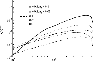
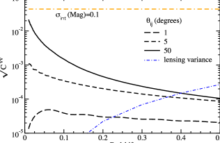
In Figure 1(a), we show the luminosity distance covariance $C^{vv}(z_{i},z_{j},\theta_{ij})$ with equal redshifts and also with $z_{i}=0.2$ for different values of $z_{j}$, as a function of the separation angle $\theta_{ij}$. In Figure 1(b) we show the covariance as a function of $z=z_{i}=z_{j}$ for several illustrative values of $\theta_{ij}$. For reference, we also plot the variance as a function of redshift $z$ and compare it to an intrinsic SN magnitude error of $\delta m=0.1$, which is the expected level to which SN light curves may be calibrated in upcoming searches. We note that the recent Supernova Legacy Survey (SNLS) has reached an average intrinsic error of 0.12 (in magnitudes). Peculiar velocities are a concern for SNe separated by angular scales of tens or more square degrees as seen in Figure 1(a), and at low redshifts, $z\lesssim 0.2$, as seen in Figure 1(b).

Figure 2: Expected errors on cosmological parameters due to the peculiar velocity covariances. In Figure 2(a) (left panel) the expected errors on a constant dark energy equation of state, $w=w_{0}$, and the matter density parameter are shown. In Figure 2(b) (right panel) the expected errors on the dark energy equation of state parameters, $w_{0}$ and $w_{1}$, where $w=w_{0}+(1-a)w_{1}$, and assuming a prior uncertainty on $\Omega_{M}$ of 0.01, are shown. We have assumed a survey of 300 SNe out to a redshift of 0.2 over 10,000 sqr. degrees, such as the Supernova Factory, and another 1700 SNe between redshifts 0.2 and 1.7 in 10 sqr. degrees on the sky, such as from SNAP/JDEM. We break the error ellipses to covariances from lensing and peculiar velocities.

To determine the impact on cosmological parameter estimates, we compute the Fisher information matrix

$${\bf F}_{\alpha\beta}=\sum_{ij}\frac{\partial d_{L}(z_{i})}{\partial p_{\alpha}}({\rm Cov}^{-1})_{ij}\frac{\partial d_{L}(z_{j})}{\partial p_{\beta}}\,.$$ (5)

If the errors are uncorrelated in the Hubble diagram, then the final error on a given cosmological parameter obtained by model fitting is $\sigma_{\rm int}/\sqrt{N(z_{i})}$. But in the case that there are correlations between data points due to bulk flows, the final error is close to $\sigma_{\rm int}\sqrt{1+[N(z_{i})-1]r^{2}}/\sqrt{N(z_{i})}$ where $r\equiv{\rm Cov}(i,j)/\sqrt{{\rm Var}(i){\rm Var}(j)}$ is the average correlation between data points. The limit $r\to 0$ corresponds to the case of uncorrelated errors, but in the limit of perfect correlation, $r\to 1$, the error remains as $\sigma_{\rm int}$ with no improvement from the number of SNe in the survey. For $0<r^{2}<1$, while there is an improvement with increasing the SNe sample size, in the limit of large numbers, the error on an individual parameter will not improve beyond $r\sigma_{\rm int}$.

Analysis.—To estimate cosmological parameter measurement errors, we consider a survey with 2000 SNe, similar to the combined Supernova Factory and the Supernova Acceleration Probe (SNAP) proposal for a JDEM. We distribute 300 SNe uniformly in redshift between 0 to 0.2 over an area of 10,000 sqr. degrees, and 1700 between redshifts 0.2 and 1.7 over 10 sqr. degrees. We calculate the covariance matrix of size 2000 by 2000 obtained by assuming a distribution of separations that peaks at roughly one half of the diagonal of the survey geometry (assumed to be a square).

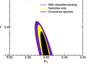
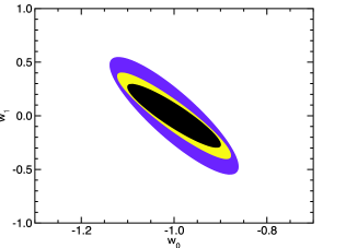
In Figure 2, we summarize our results related to cosmological parameter estimates. Here, we have considered the measurement of four parameters, the matter density parameter $\Omega_{m}$, the Hubble parameter $h$ which can also be considered as an overall normalization to the Hubble diagram (and affected by low-redshift bulk flows), and assume a dark energy equation of state given by $w(a)=w_{0}+(1-a)w_{1}$. Our fiducial test model is a cosmological constant plus cold dark matter, with $w_{0}=-1,\,w_{1}=0$ and matter density $\Omega_{m}=0.3$. In Figure 2(a), we assume $w_{1}=0$ exactly and consider the measurement of $\Omega_{m}$ and $w=w_{0}$. In Figure 2(b), we set a prior on $\Omega_{m}$ with $\sigma(\Omega_{m})=0.01$, and consider measurement of $w_{0}$ and $w_{1}$. The error ellipses show the expected errors based on which part of the covariance is included. The innermost ellipse is the case where covariance is ignored and only intrinsic noise is included while the outermost ellipse is the case where both peculiar velocities and lensing covariance are taken into account. We can see that the velocity correlations dilate the $\Omega_{m}-w_{0}$ uncertainty by $\sim 25\%$ in the case illustrated by Figure 2(a), and the $w_{0}-w_{1}$ uncertainty by $\sim 20\%$ in the case illustrated by Figure 2(b). Including the effects of both velocities and weak lensing, for which the variance rather than covariance between sources is dominant, we see that the uncertainties expand by $40\%,\,150\%$ on $w_{0},\,\Omega_{m}$ respectively in case (a), and $50\%$ on $w_{0},\,w_{1}$ in case (b).

In general, smaller separations at high redshift lead to an increase in parameter errors from lensing, while at low redshifts correlations at the scales of a few tens sqr. degrees increase the peculiar velocity contribution. A combination of large area ($\sim$ 10,000 sqr. degrees) at $z<0.2$ and a smaller area ($\sim$ a few tens sqr. degrees) at higher redshifts provides the optimal combination, though covariances are not simply reduced to zero in that case.

Figure 3: The rms fluctuations in the line-of-sight projected velocities $\sqrt{l^{2}C_{l}/2\pi}c$ in km/s as a function of the multipole. We show the angular power spectrum at different redshifts. The diagonal, dot-dashed line is the expected noise power spectrum for velocity measurements for a sample of SNe with an intrinsic uncertainty of 0.1 magnitudes and a surface density of 50 sr^-1. Along the lines of a survey such as the Supernova Factory, which expects $\sim$ 300 SNe at low redshifts, $z=0.01-0.08$, and assuming the survey to be spread over a fractional sky area $f_{\rm sky}=0.5$, we plot the expected error boxes for angular power spectrum measurements binned in multipole space, for the mean survey redshift. The velocity fluctuations are detected at the cumulative signal-to-noise ratio $\sim$ 7.

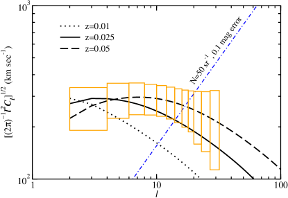
There is some possibility to use the dispersion in the Hubble diagram as a measure of peculiar velocity fluctuations. This is summarized in Figure 3, where we plot the angular power spectrum of line-of-sight projected velocities as a function of redshift in the form of rms fluctuations given by $v_{\rm rms}=\sqrt{l^{2}C_{l}/2\pi}c$. The plotted power spectrum is equivalent to the Fourier transform of Eq. (3) except that we have not included factors of $(1-a/a^{\prime}\chi)$ which relate fluctuations in the velocity field to that of the luminosity distances estimated with SNe. We are assuming that an individual distance estimate, combined with redshift and an external estimate of the overall normalization of the SN light curve, can be converted to an estimate of the peculiar velocity Miller:1992 . In Figure 3, we also show the uncertainty related to peculiar velocity fluctuation measurements, $\sigma_{\rm vel}^{2}/\bar{N}$ where $\sigma_{\rm vel}$ is the intrinsic error in the velocity measurement from each SN and $\bar{N}$ is the surface density of SNe (in sr^-1). Assuming an intrinsic uncertainty of $0.1$ magnitudes, then $\sigma_{\rm vel}=\sigma_{int}cz/2.17$ (in km/s) which at $z\sim 0.02$ is 275 km/s. We also assume no uncertainty in the observer’s velocity, and that the measurements are not limited by uncertainties in cosmological parameters such as the Hubble constant or affected by any systematic biases. At low redshifts, surveys such as the Supernova Factory expect $\sim$ 300 SNe over 2$\pi$ sr so that using an estimate of 50 sr^-1 for the surface density and $f_{\rm sky}=0.5$ for the fractional sky coverage, we obtain the expected error boxes for binned multipole measurements in Fig. 3. The line-of-sight projected velocity anisotropy power spectrum is detected with a cumulative signal-to-noise ratio of $\sim 7$ for the noise curve and error bars shown in Figure 3. However, this is not a significant detection for detailed cosmological parameter estimates. For comparison, unlike the low velocity anisotropy “signal” captured by low redshift SNe, it may be possible to study clustering statistics of lensing magnification with samples of SNe at a redshift beyond unity with signal-to-noise ratios of order thirty or more Dodelson:2005zt ; Cooray:05b .

While peculiar velocity fluctuations in the Hubble diagram do not provide extra cosmological information, there are significant implications for distance estimators and cosmological probes. For example, due to the correlations, a full $N_{\rm tot}\times N_{\rm tot}$ Fisher matrix, as opposed to a redshift-binned smaller version, is required in order to obtain cosmological parameter accuracy estimates. Presumably this is not a problem since the correct treatment of SN calibration uncertainties already requires the full $N_{\rm tot}\times N_{\rm tot}$ (or even larger) covariance matrix Kim_Miquel . The challenge is significant, however, as one can neither ignore small correlations nor assume some arbitrary cosmology to estimate covariance among measurements which are then used to extract new cosmological parameters. The full covariance matrix must be established as a function of cosmological parameters to obtain an accurate gauge of cosmological parameter uncertainty.

None of these considerations will deter upcoming searches for SNe for cosmological purposes, though a careful consideration must be given to account for velocity fluctuations at low redshifts and lensing effects at high redshifts. Since peculiar velocity correlations are only significant at $z<0.2$, one can potentially ignore low redshift SNe when fitting distance data to cosmological estimates. In this case, we find that the parameter errors are not significantly affected by velocity correlations except that the errors are increased by the fractional factor in which the SN sample is reduced. In fact, this increase is larger than the case where all SNe are used to estimate cosmology, but with a proper accounting of the correlations. So, instead of simply throwing away data, such as low-redshift SNe, it may be best to keep the sample as a whole, but develop techniques to account for peculiar velocity correlations.

Since the low, $\ell\leq 6$ multipoles in the velocity anisotropy spectrum dominate the SN distance covariance, if such multipoles can be determined independently of the SN measurements then corrections, at least partially, can be applied to the interpretations of the Hubble diagram. If a signal-to-noise ratio of 10 measurement in each multipole is adequate for a reasonable correction, then independent bulk flow measurements at redshifts ranging over 0.01 to 0.1 must involve a source surface density of $10^{3}$ sr^-1 and an uncertainty in the velocity measurement of each object below 100 km s^-1. Such a surface density of sources and a velocity error may be achievable with cluster studies of the kinetic Sunyaev-Zeld́ovich SZpaper effect with the upcoming Planck surveyor (http://www.rssd.esa.int/index.php?project=PLANCK), though foregrounds and internal motions within clusters will contaminate bulk flow measurements and reduce the overall signal-to-noise ratio levels Holder:2002wc . Another approach will be to consider information from an almost all-sky peculiar velocity survey based on low-redshift galaxy samples. In the past, the IRAS Point Source Redshift Catalog (PSCz) has allowed modeling of the spherical harmonic moments of the velocity field Teodoro:2003ur out to a redshift of 0.02. We encourage the development of techniques to use information from such surveys to correct the correlations in the low redshift part of the Hubble diagram.

Figure 4: Correlations in the Hubble constant, $C^{HH}(z_{1},z_{2},\theta)$, as a function of $\theta$ when $z_{1}=z_{2}$. At redshifts less than 0.05, the correlations are generally at the level of few times $10^{-4}$ and peak at angular scales of $50^{\circ}$, suggesting that the Hubble constant should show fluctuations at the level a few percent, at most, when divided to patches on the sky at the same angular scale. A reliable detection of this few percent fluctuation is challenging given the low surface density of SNe expected at low redshifts, similar to the detection of velocity anisotropies shown in Figure 3.

It is interesting to note that the dimensionless fluctuations of the angular-diameter distance $d_{A}$ due to large-scale bulk motions are identical to that for the luminosity distance,

$$\delta d_{A}/d_{A}=\delta d_{L}/d_{L}.$$ (6)

This means our results for velocity covariances apply equally to distances based on angular-diameter measurements. Possible scenarios include the distances to large scale structure obtained through baryon acoustic oscillations Eisenstein:2005su , distances to galaxies using the Sunyaev-Zeld́ovich effect (for a recent example, see Bonamente:2005ct ) or other features such as radio lobes Daly:2003iy ; Jackson:2003jw , and probes of cosmology using the Alcock-Pazcynski APtest test which employ the angular-diameter distance to a correlation radius. The survey details will differ in all cases, so that the extent to which velocity correlations of low-redshift, wide-separation objects contribute noise will also vary.

We can also consider dimensionless fluctuations of the Hubble constant, inferred from either luminosity or angular-diameter distances. Using $d_{L}$, we note that $H^{-1}=d/dz[d_{L}/(1+z)]$ whereby

$$\frac{\delta H}{H}=-\frac{\delta d_{L}}{d_{L}}+\chi\frac{d}{d\eta}\left(\frac{\delta d_{L}}{d_{L}}\right).$$ (7)

The second term on the right includes the correction due to the peculiar acceleration. At low redshifts, this is equivalent to $\delta_{H}=-\delta_{d_{L}}+\delta_{z}(1+\frac{1}{2}(1-q)z+{\cal O}(z^{2})),$ which we obtain by perturbing the redshift expansion of the luminosity distance. Here, $\delta_{X}$ is the fractional perturbation to $X=H,\,d_{L},\,z$ and $\delta_{z}=(1+1/z)\hat{\bf n}\cdot({\bf v_{\rm SNe}}-{\bf v_{\rm obs}})$. (See Refs. Sugiura ; Hui .) In principle, the deceleration parameter $q$, also varies on the sky and suffers from correlations. Similar to fluctuations associated with distance in Eq. (Large-Scale Bulk Motions Complicate the Hubble Diagram), one can define a covariance for the Hubble constant anisotropies using the line-of-sight projected correlation function for the velocity field. This covariance is

$$C^{HH}(z_{i},z_{j},\theta_{ij})=\sum_{\rm even\;\;\ell}\frac{2l+1}{4\pi}\cos\theta_{ij}\frac{2}{\pi}F_{l}$$

$$\times \int dkP_{mm}(k,z_{i},z_{j})j_{l}(k[\chi_{i}-\chi_{j}\cos\theta_{ij}])j_{l}(k\chi_{j}\sin\theta_{ij})$$

$$\times \left\{{D}^{\prime}(z_{i})\left(1-\frac{a}{a^{\prime}\chi}\right)_{i}+\chi_{i}\left[{D}^{\prime}(z_{i})\left(1-\frac{a}{a^{\prime}\chi}\right)_{i}\right]^{\prime}\right\}$$

$$\times \left\{{D}^{\prime}(z_{j})\left(1-\frac{a}{a^{\prime}\chi}\right)_{j}+\chi_{j}\left[{D}^{\prime}(z_{j})\left(1-\frac{a}{a^{\prime}\chi}\right)_{j}\right]^{\prime}\right\},$$

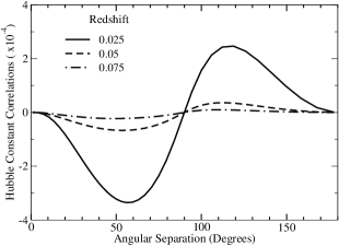
where $F_{l}$ is defined below Eq. (Large-Scale Bulk Motions Complicate the Hubble Diagram). Compared to fluctuations of the luminosity distance, anisotropies in the Hubble constant are larger by a factor of $\sim 3-5$ depending on the redshift and the deceleration parameter (see Figure 4). The increase comes from the correction to fluctuations associated with peculiar acceleration in Eq. (7). As shown in Figure 4, at redshifts between 0.025 to 0.05, fluctuations in the Hubble constant are at most a few percent, given that the correlations are $C^{HH}(z_{i},z_{j},\theta_{ij})\sim{\cal O}(10^{-4})$ at angular scales of 60 degrees. Detecting such a small fluctuation from a low redshift SN survey such as the Supernova Factory, however, will be challenging just as velocity fluctuations are marginally measurable from SN surveys. This is mostly due to the low surface density of SNe expected at low redshifts.

Note that the expressions for the Hubble constant and distance fluctuations depend on the line-of-sight source and observer velocities separately. Hence, there is the possibility of a “Hubble bubble,” large fluctuations in $H$, if the motion of the reference frame defined by the sources, SNe or large scale structure, does not converge to our reference frame, defined relative to the cosmic microwave background Davis:1983 ; Tammann:1990 ; Sandage:1990 ; Turner:1992 . For example, a local low-density bubble could bias $H$ high by $\sim 5\%$ Wang:1997tp ; Zehavi:1998gz , although observations suggest that the reference frames have indeed converged by length scales $\sim 50$ Mpc/h Giovanelli:1999 ; Riess:2005zi . Nevertheless, our local motion will induce correlated velocity fluctuations if it is not removed from the data properly.

To conclude, we have investigated the correlated distortions of the luminosity distance-redshift relation due to large-scale bulk flows and how these correlations limit the precision with which cosmological parameters can be measured. At low redshifts, peculiar velocities correlate errors of type 1a SNe and prevent a precise calibration of the Hubble diagram, relative to the scenario where one arbitrarily assumes no correlations so that the errors decrease by the square-root of the number of SNe. The increase in individual error of a distant SN, or the correction to variance from the velocity field, however, is negligible relative to an expected intrinsic error of 0.1 to 0.15 magnitudes. These results are consistent with other recent calculations on how peculiar velocities affect cosmological studies with SNe Hui . Turning our arguments around, we find that the measurement of large-scale bulk flows at low redshifts using SN distance indicators is challenging. At high redshifts, weak gravitational lensing magnification adds an extra dispersion to the light curve and increases the individual errors of SN distance estimates. For surveys that are concentrated on smaller areas on the sky, weak lensing also correlates distance estimates, but the increase in individual variances generally dominates the error budget. We also considered similar distortions of the angular-diameter distance, as well as the Hubble constant.