Abstract

The galactic environment of the Sun varies over short timescales as the Sun and interstellar clouds travel through space. Small variations in the dynamics, ionization, density, and magnetic field strength in the interstellar medium (ISM) surrounding the Sun can lead to pronounced changes in the properties of the heliosphere. The ISM within $\sim$30 pc consists of a group of cloudlets that flow through the local standard of rest with a bulk velocity of $\sim$17–19 km s^-1, and an upwind direction suggesting an origin associated with stellar activity in the Scorpius-Centaurus association. The Sun is situated in the leading edge of this flow, in a partially ionized warm cloud with a density of $\sim$0.3 cm^-3. Radiative transfer models of this tenuous ISM show that the fractional ionization of the ISM, and therefore the boundary conditions of the heliosphere, will change from radiative transfer effects alone as the Sun traverses a tenuous interstellar cloud. Ionization equilibrium is achieved for a range of ionization levels, depending on the ISM parameters. Fractional ionization ranges of $\chi$(H)=0.19–0.35 and $\chi$(He)=0.32–0.52 are found for tenuous clouds in equilibrium. In addition, both temperature and velocity vary between clouds. Cloud densities derived from these models permit primitive estimates of the cloud morphology, and the timeline for the Sun’s passage through interstellar clouds for the past and future $\sim$10⁵ years. The most predictable transitions happen when the Sun emerged from the near vacuum of the Local Bubble interior and entered the cluster of local interstellar clouds flowing past the Sun, which occurred sometime within the past 140,000 years, and again when the Sun entered the local interstellar cloud now surrounding and inside of the solar system, which occurred sometime within the past 44,000 years, possibly a 1000 years ago. Prior to $\sim$140,000 years ago, no interstellar neutrals would have entered the solar system, so the pickup ion and anomalous cosmic ray populations would have been absent. The tenuous ISM within 30 pc is similar to low column density observed globally. In this chapter, we review the factors important to understanding short-term variations in the galactic environment of the Sun. Most ISM within 40 pc is partially ionized warm material, but an intriguing possibility is that tiny cold structures may be present.

[Short-term Variations in the Galactic Environment of the Sun]Short-term Variations in the
Galactic Environment of the Sun Short-term Variations in Galactic Environment and

Table of Contents:

6.1	Overview	2
6.2	The Solar Journey through Space: The Past $10^{4}$ to $10^{6}$ Years	14
6.3	Neighborhood ISM: Cluster of Local Interstellar Clouds	19
6.4	Radiative Transfer Models of Partially Ionized Gas	32
6.5	Passages through Nearby Clouds	38
6.6	The Solar Environment and Global ISM	43
6.7	Summary	50
	References	52

1 Overview

In 1954 Spitzer noted that the “Study of the stars is one of [mankind’s] oldest intellectual activities. Study of the matter between stars is one of the youngest.” Comparatively, the study of interstellar matter (ISM) at the heliosphere is an infant. Still younger is the study of the interaction between the heliosphere and ISM that forms the galactic environment of the Sun. The total pressure of the ISM at the solar system is counterbalanced by the solar wind ram pressure, but since both the Sun and clouds move through space, this balance is perturbed as the Sun passes between clouds with different velocities or physical properties. In this chapter, we focus on variations in the galactic environment of the Sun over timescales of $\pm$3 Myrs, guided by data and models of local interstellar clouds. In essence, we strive to provide a basis for understanding the “galactic weather” of the solar system over geologically short timescales, and in the process discover recent changes in the Sun’s environment that affect particle populations inside of the heliosphere, and perhaps the terrestrial climate. The heliosphere, the bubble containing the solar wind plasma and magnetic field, dances in the wind of interstellar gas drifting past the Sun. This current of tenuous partially ionized low density ISM has a velocity relative to the Sun of $\sim$26 km s^-1. It would have taken less than 50,000 years for this gas to drift from the vicinity of the closest star $\alpha$ Cen, near the upwind direction in the local standard of rest (LSR, Tables 1), and into the solar system.

Star formation disrupts the ISM. The nuclear ages of massive nearby stars in Orion (at a distance of $\sim 400$ pc) and Scorpius-Centaurus (at $\sim 150$ pc) are 4-15 Myr, so the solar system has been bombarded by high energy photons and particles many times over the past 10⁷ years. Recent nearby supernova events include the formation of the Geminga pulsar $\sim 250,000$ years ago, and possibly the release of $\zeta$ Oph as a runaway star $\sim$0.5-1 Myr ago. The dynamically evolving interstellar medium inhibits the precise description of the solar Galactic environment on timescales longer than $\sim 1-3$ Myrs.

Variations in the galactic environment of the Sun for time scales of $\sim$3 Myrs are short compared to the vertical oscillations of the Sun through galactic plane, and short compared to the disruption of local interstellar clouds by star formation. The oscillation of the Sun in the Galactic gravitational potential carries the Sun through the galactic plane once every $\sim 34$ Myrs, and the Sun will reach a maximum height above the plane of $\sim 78$ pc in about 14 Myrs ([Bash, 1986, Vandervoort and Sather, 1993], also see Chapter 5 by Shaviv). The motion of the Sun compared to the kinematics of some ensemble of nearby stars is known as the solar apex motion, which defines a hypothetical closed circular orbit around the galactic center known as the Local Standard of Rest (LSR, §1.2). Note that the LSR definition is sensitive to the selection of the comparison stars, since the mean motions and dispersion of stellar populations depend on the stellar masses. The transformation of the solar trajectory into the LSR for comparison with spatially defined objects, such as the Local Bubble, introduces uncertainties related to the LSR.

A striking feature in the solar journey through space is the recent emergence of the Sun from a near vacuum in space, the Local Bubble, with density $\rho<10^{-26}$ g cm^-3 ([Frisch, 1981, Frisch and York, 1986], §2). We will show that the Sun has spent most of the past $\sim$3 Myrs in this extremely low density region of the ISM, known as the Local Bubble. The Local Bubble extends to distances of over 200 pc in parts of the third galactic quadrant ($l=180^{\circ}\rightarrow 270^{\circ}$, [Frisch and York, 1983]), and is part of an extended interarm region between the Sagittarius/Carina and the Perseus spiral arms. The proximity of the Sun to the Local Bubble has a profound effect on the solar environment, and affects the local interstellar radiation field, and dominates the historical solar galactic environment of the Sun (§2.2). Neutral ISM was absent from the bubble, and byproducts of the ISM-solar wind interaction, such as dust, pickup ions and anomalous cosmic rays, would have been absent from the heliosphere interior.

The Local Bubble is defined by its geometry today, so the solar space motion is a variable in estimating the departure of the Sun from this bubble. For all reasonable solar apex motions, sometime between 1000 and 140,000 years ago the Sun encountered material denser than the nearly empty bubble. During the late Quaternary geological period, the Sun found itself in a flow of warm low density ISM, $n\sim 0.3$ cm^-3, originating from the direction of the Scorpius-Centaurus Association (§§3, 6.4). The Sun is presently surrounded by this warm, $T\sim 7,000$ K, tenuous gas, which is similar to the dominant form of ISM in the solar neighborhood. The physical characteristics of this cluster of local interstellar cloudlets (CLIC) are discussed in §3.

Figure 1: SEE fig1a.pdf and fig1b.pdf. The solar position and motion are compared to the Local Bubble for two planes aligned with the solar apex motion (Table 1). The left figure gives the Local Bubble ISM distribution in a plane that is tilted by 27^∘ to the Galactic plane with the northern surface normal pointing towards (220^∘, $+$63^∘). Stars with latitudes within about $\pm$15^∘of that plane are plotted. The right figure shows a meridian slice perpendicular to the galactic plane, and aligned with the $\ell$=40^∘— 220^∘ axis. Stars with longitudes within $\pm$25^∘ of the meridian slice are plotted. These ISM distributions were constructed from cleaned and averaged photometric and astrometric data for O, B, and A stars in the Hipparcos catalog. For a solar LSR velocity of $13-20$ pc/Myrs, the Sun has been within the Local Bubble for over 3 Myrs. The symbols show $E(B-V)$ values 0.017–0.051 mag (tiny x’s), 0.051–0.088 mag (boxes), 0.088–0.126 mag (dots), and $>0.126$ mag (triangles) so that shading levels give $N$(H)$\sim 10^{20.4}\rightarrow 10^{20.7},\leavevmode\nobreak\ \sim 10^{20.7}\rightarrow 10^{20.9},\leavevmode\nobreak\ \mathrm{and}>10^{20.9}$, after assuming N(H^o+2H₂)/$E(B-V)$=21.76 cm^-2mag^-1. The solar motion is shown for both Standard and Hipparcos values. The large intensely shaded triangles show dust clouds from Dutra and Bica (2002). The CLIC column densities are below the minimum value of $N$(H^o)$\sim 10^{20.40}$ cm^-2 displayed here.

The solar entry into the CLIC would correspond to the appearance of interstellar dust, pickup ions and anomalous cosmic rays in the heliosphere. The dust filtration by the solar wind and in the heliosheath is sensitive both to dust mass and the phase of the solar cycle (see Landgraf chapter), so that these two effects are separable. In principle the solar journey through clouds could be traced by comparative studies of interstellar dust settling onto the surfaces of inner versus outer moons.

In §5.2 we discuss the Sun’s entry into, and exit from, the interstellar cloud now surrounding the solar system, and show that it can be determined from a combination of data and theoretical models. The velocity of this cloud, known as the local interstellar cloud (LIC), has been determined by observations of interstellar He^o inside of the solar system ([Witte, 2004]). We test several possibilities for the three-dimensional (3D) shape of the LIC, and conclude that the Sun entered the surrounding cloud sometime within the past 40,000 years, and possibly very recently, in the past $\sim$1000 years.

The velocity difference between interstellar He^o inside of the solar system, and interstellar D^o, Fe⁺ and other ions towards stars in the upwind direction, including the nearest star $\alpha$ Cen, together indicate the Sun will emerge from the cloud now surrounding the Sun within $\sim$4,000 years. This raises the question of “What is an interstellar cloud?”, which is difficult to answer for low column density ISM such as the CLIC, where cloudlet velocities may blend at the nominal UV resolution of 3 km s^-1.

Determining the times of the solar encounter with the LIC, and other clouds, requires a value for $n$(H^o) in the cloud because distance scales are determined by $N$(H^o)/$n$(H^o). Theoretical radiative transfer models of cloud ionization provide $n$(H^o) and $n({\rm H^{+}})$ for tenuous ISM such as the LIC, and supply important boundary constraints for heliosphere models. CLIC column densities are low, $N$$\ {\raise-2.15277pt\hbox{$\buildrel<\over{\sim}$}}\ 10^{18}$, and radiative transfer effects are significant (§4). Models predict $n$(H^o)$\sim$0.2 cm^-3 and $n({\rm H^{+}})$$\sim$0.1 cm^-3 at the Sun, with ionization levels rising slowly to the cloud surface so that $\langle n$(H^∘)$\rangle_{\mathrm{LIC}}$$\sim$0.17 cm^-3.

In §6.1 we discuss the relative significance of diffuse warm partially ionized gas (WPIM) and traditional Strömgren spheres for the heliosphere. Distinct regions of dense fully ionized ISM are infrequent near the Sun, although regions of ionized gas surround distant massive stars bordering the Local Bubble, and surround $\beta$ Cen and $\lambda$ Sco, which helps energize the Loop I superbubble interior. The Sun’s path is unlikely to traverse, or have traversed, an H II region around an O–B1 star for $\pm$4 Myrs because no such stars or H II regions are within 80 pc of the Sun. Hot white dwarf stars are more frequent nearby, and may in some cases be surrounded by small Strömgren spheres. In contrast, diffuse ionized gas is widespread and has been observed extensively using weak optical recombination lines from ${\rm H^{+}}$ and other species, synchrotron emission, and by the interaction of pulsar wave packets with ionized interstellar gas. The CLIC and diffuse ionized gas are part of a continuum of ionization levels predicted and observed for low density interstellar gas.

The heliosphere should vary over geologically short timescales, for reasons unrelated to the Sun or solar activity, when encountering the small scale structure of the nearby ISM. These variations in the cosmic environment of the Sun may be traced by terrestrial radioisotope records, or by variable fluxes of interstellar dust grains deposited on planetary moons (see other chapters in this volume). Over 3 Myrs timescales the Sun travels 40-60 pc through the LSR, and the interval between cloud traversals should be less than $\leq 80,000$ years. Differing physical properties of cloudlets in the flow will affect the heliosphere and interplanetary medium. If cloud densities are relatively uniform at $n$(H^o)$\sim$0.2 cm^-3, then data on ISM towards nearby stars indicate these clouds fill $\sim$33% of space within 10 pc, with mean cloud lengths of $\sim 1.0$ pc, and with a downwind hemisphere that is emptier than the upwind hemisphere (§3.3).

The ISM within $\sim$2 pc is inhomogeneous. The ratio Fe⁺/D^o increases as the viewpoint sweeps from the downwind to upwind direction, signaling either grain destruction in an upwind interstellar shock, or increased cloud ionization. The Fe⁺/D^o gradient is consistent with the destruction of CLIC dust grains in a fragment of the expanding superbubble around the Scorpius-Centaurus Association (§6.4). There are several possibilities for the next cloud to be encountered, and the most likely candidate is the cloud towards the nearest star $\alpha$ Cen (§5.3), where only modest consequences for the heliosphere are expected, since the temperature and velocity of the cloud differ only by $\sim$800 K and $\sim$3 km s^-1, respectively.

The properties of the CLIC are similar to low column density ISM observed in the solar vicinity, and observed in the Arecibo Millennium survey of very low $N$(H^o) clouds ([Heiles and Troland, 2004]). The warm neutral medium (WNM) in the Arecibo survey appears to be similar to the CLIC, but so far, counterparts of the exotic cold, low column density, neutral clouds, $T\sim 50$ K and $N$(H^o)$\sim 10^{18}$ cm^-2, are not found locally (§6). If they are hidden in the upwind ISM, they would be far from ionization equilibrium (having much lower ionization than the surrounding warm, ionized gas), in contrast to the LIC gas (§4). Cold ISM towards 23 Ori indicate densities of $>$10 cm^-3 for the cold neutral medium gas (CNM).

We do not discuss high-velocity, $v\sim 100$ km s^-1, low column density radiative shocks. Such disturbances would cross the heliosphere on timescales of $\sim 5-10$ years, seriously perturbing it ([Sonett et al., 1987, Frisch, 1999, Mueller et al., 2005]), and would be evolving as they cool. Low column density high velocity shocked gas, $N$(H)$\sim 10^{16}-10^{17}$ cm^-2, $n_{\rm o}$$\sim$0.5–5 cm^-3, could be common in ISM voids. However, with high velocities of $\sim$100 km s^-1, such gas will traverse voids such as the Local Bubble in less than 1 Myr. Similar high-velocity gas is associated with the Orion’s Cloak superbubble shell around Orion and Eridanus, with $v\sim 100$ km s^-1 and $N$(H)$\sim 10^{16}-10^{17}$ cm^-2 ([Welty et al., 1999]). Rapidly moving low column density shocks similar to these would pass over the heliosphere quickly, in 50 – 1,500 years, with strong implications for heliosphere structure (Zank et al., this volume). The fairly coherent velocity and density structure and relatively weak turbulence in the CLIC argues against any such disturbance having occurred recently (see §3.4). We also do not discuss dense molecular clouds, which are discussed in the Shaviv chapter.

As a way of summarizing short term solar environment, we show the solar position inside of the Local Bubble in Figure 1 (see 2.1). We will now briefly review relevant fundamental material.

1.1 Fundamental Concepts

Basic concepts needed for understanding the following discussions are summarized here. We use the local standard of rest, LSR, based on the Standard solar motion, unless otherwise indicated. Velocities quoted as heliocentric (HC) are with respect to the Sun, while LSR velocities are obtained by correcting for the motion of the Sun with respect to the nearest stars, or the solar apex motion. The basic principles underlying obtaining the properties of interstellar clouds are summarized in §1.3.

The ultraviolet and X-ray parts of the spectrum play an essential role in the equilibrium of interstellar clouds. The spectral regions relevant to the following discussions are the ultraviolet (UV), with wavelengths $1200\,\mathrm{{\cm10pt\AA}}<\lambda<3000\,\mathrm{{\cm10pt\AA}}$; the far ultraviolet (FUV), $912\,\mathrm{{\cm10pt\AA}}<\lambda<1200\,\mathrm{{\cm10pt\AA}}$; the extreme ultraviolet (EUV), $100\,\mathrm{{\cm10pt\AA}}<\lambda<912\,\mathrm{{\cm10pt\AA}}$; and the soft X-ray, $\lambda<100\,$Å. The spectrum of the soft X-ray background (SXRB), photon energies $<0.5$ keV, has been an important diagnostic tools for the distribution of ISM with column density $N$(H^o)$>10^{19.5}$ cm^-2. The first ionization potential (FIP) of an atom is the energy required to ionize the neutral atom. The FIP of H is 13.6 eV. Elements with FIP $<13.6$ eV are predominantly ionized in all clouds, since the ISM opacity to photons with energies $E<13.6$ eV is very low. The ionization potential, IP, of several ions are also important. For instance IP(Ca⁺)=11.9 eV, and $N$(Ca⁺⁺)/$N$(H^o) may be large in warm clouds. For $T>4,000$ K and $n{\rm(e)}$$<$0.13 cm^-3, Ca⁺⁺/Ca⁺$>$1. Variations in the spectrum of the ionizing radiation field, as it propagates through a cloud caused by the wavelength dependence of the opacity, $\tau(\lambda)$, are referred to as radiative transfer (RT) effects.

Color excess is given by $E(B-V)$, and represents the observed star color, in magnitudes, measured in the UBV system, compared to intrinsic stellar colors (e.g. [Cox, 2000]). Color excess represents the intrinsic star color combined with reddening by foreground dust. The column density, $N$(X), is the number of atoms X contained in a column of material with a cross section of 1 cm^-2 and bounded at the outer limit by an arbitrary point such as a star. The volume density, $n$(X), is the number of atoms cm^-3. The notation $n_{HI,0.2}$ indicates the H^o space density in units of 0.2 cm^-3. The fractional ionization of an element X is $N{\rm(X^{+})}$/($N{\rm(X^{\circ})}$+$N{\rm(X^{+}))}$. The filling factor, $f$, gives the percentage of the space that is filled by ISM denser than the hot gas in the Local Bubble (i.e. warm or cold gas).

Among the various acronyms we use are the following: The interstellar cloud feeding neutral ISM and interstellar dust grains (ISDG) into the solar system is the local interstellar cloud (LIC). A cluster of local interstellar clouds (CLIC) streams past the Sun, forming absorption lines in the spectra of nearby stars. Alternative names for the CLIC are the “Local Fluff” and the very local ISM, and the LIC is a member of the CLIC. The upwind portion of the CLIC has been called the “squall line” ([Frisch, 1995]). In the global ISM we find cold neutral medium (CNM), warm neutral medium (WNM), and warm ionized medium (WIM). Both observations and our radiative transfer models of tenuous ISM, $N$(H)$\ {\raise-2.15277pt\hbox{$\buildrel<\over{\sim}$}}\ 10^{18}$ cm^-2, indicate that warm partially ionized medium (WPIM) is prevalent nearby.

The Scorpius-Centaurus Association (SCA) is a region of star formation that dominates the distribution of the ISM in the upwind direction of the CLIC flow, including the Loop I supernova remnant. The Local Bubble (LB) is a cavity in the interstellar dust and gas around the Sun that may merge in some regions with the bubble formed by stellar evolution in the SCA, Loop I, near the solar location ([Frisch, 1995]). The Local Bubble is used here to apply to those portions of nearby space, within $\sim$70 pc, with densities $\rho<10^{-26}$ g cm^-3.

The densities of neutral interstellar gas at the solar location are provided by data on pickup ions (PUI) and anomalous cosmic rays (ACR). PUIs are formed from interstellar neutrals inside the heliosphere, which have become ionized and captured by the solar wind (Moebius et al., this volume). ACRs are PUIs that are accelerated in the solar wind and termination shock to energies of $\leq$1 GeV/nucleon (Fahr et al., Florinski et al., this volume).

Element abundances in the CLIC gas are similar to warm gas in the Galactic disk, and the missing atoms are believed to be incorporated in dust grains ([Frisch et al., 1999, Welty et al., 1999]). We will assume that the solar abundance pattern provides the benchmark abundance standard for the local ISM, although this issue has been debated ([Snow, 2000]), and although the solar abundance of O and other elements are controversial (e.g. [Lodders, 2003]). Using solar abundances as a baseline, the depletion $\delta$ of an element represents the amount of the element that is missing from the gas. Depletion is defined as $\delta_{\rm X}={\rm log}\leavevmode\nobreak\ \frac{[{\rm X}]_{\rm ISM}}{[{\rm X}]_{\rm Solar}}$ for an element X with abundance $[{\rm X}]$ ([Savage and Sembach, 1996]). The depletion and condensation temperature of an element correlate fairly well. This is shown by the three observed interstellar depletion groups $\delta_{\mathrm{T}i,Ca}\sim-3.3$, $\delta_{\mathrm{F}e,Cr,Co,Ni,V}\sim-2.3$, and $\delta_{\mathrm{M}g,Si}\sim-1.3$, which condense at temperatures of $\sim 1,500$ K, $\sim 1,330$ K, and $\sim 1,300$ K respectively during mineral formation in an atmosphere of solar composition and pressure ([Ebel, 2000]). The interstellar gas-to-dust mass ratio and grain composition can be reconstructed from the atoms missing from the gas phase ([Frisch et al., 1999]). Depletions vary between warm tenuous and cold dense ISM, an effect originally parameterized by velocity and known as the Routly-Spitzer effect ([McRae Routly and Spitzer, 1952]), and now attributed to partially ionized warm ISM that has been shocked (§4.3). The largest variations are found for refractory elements, and result from ISDG destruction by interstellar shocks ([Jones et al., 1994, Slavin et al., 2004]). Depletion estimates are sensitive to uncertainties in $N$(H), which in cold clouds must include $N$(H₂) , and in warm tenuous clouds must include ${\rm H^{+}}$, both of which can be hard to directly measure.

Satellites that have revolutionized our understanding of the galactic environment of the Sun include Copernicus, the International Ultraviolet Explorer, IUE, the Extreme Ultraviolet Explorer, EUVE, the shuttle launched Interstellar Medium Absorption Profile Spectrograph, IMAPS, the Far Ultraviolet Explorer, FUSE, and the Hubble Space Telescope, HST (with the Goddard High Resolution Spectrometer, GHRS, and the Space Telescope Imaging Spectrograph, STIS).

Several papers in the literature have provided important insights to the physical properties of the local ISM, and are referred to throughout. Among them are: Frisch (1995, hereafter F95), which reviews the physical characteristics of the Local Bubble and the CLIC; Gry and Jenkins (2001, hereafter GJ) and Hebrard et al. (1999), which present the physical characteristics of the two nearby interstellar clouds observed in the downwind direction, the LIC and blue-shifted cloud; Slavin and Frisch (2002, hereafter SF02) and Frisch and Slavin (2003, 2004, 2005, hereafter FS), which present detailed radiative transfer model calculations of the surrounding ISM; Frisch et al. (2002, hereafter FGW), which probes the kinematics of nearby ISM; and a series of papers by Redfield and Linsky (2000, 2002, 2003, 2004, hereafter RL,), and Wood et al. (2005, hereafter W05), which assemble a wide range of UV data on the CLIC. Recent papers presenting results from FUSE also contribute significantly to our understanding of the tenuous ISM close to the Sun.

1.2 The Solar Apex Motion and Local Standard of Rest

Comparisons between the solar position and spatially defined objects, such as the LB, require adoption of a velocity frame of reference. The “Local Standard of Rest” (LSR) represents an instantaneous inertial frame for a corotating group of nearby stars ($<$500 pc) on a closed circular orbit around the galactic center, and is commonly used for this purpose. The solar motion with respect to the LSR, known as the solar “apex motion”, is dynamically defined with respect to a sample of nearby stars. All reasonable values for the LSR indicate that the Sun is traveling away from the ISM void in the third quadrant of the Galaxy, $\ell$=180^∘$\rightarrow$ 270^∘, at a velocity of $\sim$13–20 pc/Myrs.

The Sun is $\sim$8 kpc from the galactic center. The mean orbital motion around the galactic center of nearby stars is $\sim$220 km s^-1, and the solar velocity is 225$\pm$20 km s^-1 (e.g., see proper motion studies of extragalactic radio sources beyond the galactic center, [Reid et al., 1999]). Accurate astrometric data for stars is provided by the $Hipparcos$ catalog of proper motions and positions of $\sim$120,000 nearby stars ([Perryman, 1997]). For the coordinate system $\hat{x}$, $\hat{y}$, $\hat{z}$, which represent unit vectors towards the galactic center, direction of galactic rotation, and north galactic pole respectively, the speeds $V_{\rm x}$, $V_{\rm y}$, and $V_{\rm z}$ then represent the mean solar velocity in the $\hat{x}$, $\hat{y}$, and $\hat{z}$, directions compared to some arbitrarily selected set of nearby stars. A kinematically unbiased set of stars from the Hipparcos Catalog shows that the mean vertical and radial components of nearby star velocities have no systematic dependence on stellar mass ([Dehnen and Binney, 1998]). However $V_{\rm y}$ determined for stars hotter than A0 ($B-V<$0.0 mag) exceeds the mean LSR by $\sim$6 km s^-1, and the velocity dispersion for these relatively young stars is smaller than for evolved low mass stars. Since molecular clouds may share the motions of massive stars, the result is a lack of clarity concerning the best LSR transformation for studying the solar motion with respect to spatially defined objects.

The general practice is to transform radio data into the LSR velocity frame using the “Standard” solar motion, which is based on the weighted mean velocity for different populations of bright nearby stars irrespective of spectral class. The velocity of the Sun with respect to the Standard LSR (LSR_Std) is ($V_{\rm x}$, $V_{\rm y}$, $V_{\rm z}$)=(10.4, 14.8, 7.3) km s^-1 ([Mihalas and Binney, 1981]), giving a solar apex motion, of 19.5 km s^-1 towards $l$=56^∘, $b$=+23^∘ (or LSR_Std, Table 1). The solar motion with respect to a kinematically unbiased subsample of the Hipparcos catalog (omitting stars with $B-V<0.0$ mag) is ($V_{\rm x}$,$V_{\rm y}$,$V_{\rm z}$)=(10.0,5.3, 7.2) km s^-1, corresponding to a solar speed of $V$=13.4 km s^-1 towards the apex direction $\ell$=27.7^∘ and $b$=32.4^∘ km s^-1 (or LSR_Hip).

Table 1: The LSR Velocities of the Sun and Nearby Interstellar Clouds

	HC	LSRStd	LSRHip
	$V$, $\ell$ $b$	$V$, $\ell$ $b$	$V$, $\ell$ $b$
	(km s-1, ∘ ∘)	(km s-1, ∘ ∘)	(km s-1, ∘ ∘)
Sun	…	19.5, 56∘ 23∘	13.4, 27.7∘ 32.4∘
CLIC	–28.1$\pm$4.6, 12.4∘ 11.6∘	–19.4, 331.0∘ –5.1∘	–17.0, 357.8∘ –5.1∘
LIC	–26.3$\pm$0.4, 3.3∘ 15.9∘	–20.7, 317.8∘ –0.5∘	–15.7, 346.0∘ 0.1∘
GC	–29.1, 5.3∘ 19.6∘	–21.7, 323.6∘ 6.3∘	–17.7, 351.2∘  8.5∘
Apex	–35.1, 12.7∘ 14.6∘	–24.5, 341.3∘ 3.4∘	–23.3, 5.5∘ 4.1∘

Notes: The first row lists the Standard and Hipparcos values for the solar apex motion (§1.2). The LIC, CLIC, GC (G-cloud), and Apex velocity vectors refer to the upwind direction. Columns 2, 3, and 4 give the heliocentric velocity vector, and the LSR velocities using corrections based on the Standard and Hipparcos-derived solar apex motions, respectively.

1.3 Finding Cloud Physics from Interstellar Absorption Lines

Sharp optical and UV absorption lines, formed in interstellar clouds between the Sun and nearby stars, are the primary means for determining the physical properties of the CLIC. UV data provide the best look at cloud physics because resonant absorption transitions for the primary ionization state of many abundant elements fall in the UV portion of the spectrum. However, results based on UV data are limited by a spectral resolution, which typically is   $\buildrel>\over{\sim}$  3.0 km s^-1, and are unable to resolve the detailed cloud velocity structure seen in high resolution (typically $\sim$0.3–0.5 km s^-1) optical data. Ultimately high resolution UV data, $R\sim$300,000, are required to probe the CLIC velocity structure and to separate the thermal and turbulent contributions to absorption line broadening. The details of interpreting absorption line data can be found in Spitzer (1978); see alternatively the classic application of the “curve of growth” technique to the ISM towards $\zeta$ Oph ([Morton, 1975]).

The classic target objects for ISM studies are hot rapidly rotating O, B and A stars, where sharp interstellar absorption features stand out against broad stellar lines. However O and B stars are relatively infrequent nearby, and interstellar line data can be contaminated by sharp lines formed in circumstellar shells and disks around some A and B stars. Hence care is required to separate ISM and circumstellar features (e.g. [Ferlet et al., 1993]). White dwarf stars of DA and DO spectral types provide a hot far UV continuum that can, in many cases, be observed in the interval 912–1200 Å (e.g. [Lehner et al., 2003]). Cool stars are very frequent, and there are $\sim 30$ times more G and K stars than A stars. The cool stars have a weak UV flux and active chromospheres. Strong chromospheric emission lines can be used as continuum sources for interstellar absorption lines, although great care is required in the analysis (e.g. [Wood et al., 2005]). The disadvantage of cool stars is that uncertainties arise from blending of the interstellar absorption and stellar chromosphere emission features. For example, only the Sun has an unattenuated H^o Lyman-$\alpha$ emission feature, and its strength and shape vary with the phase of solar magnetic activity cycle. Heeding these limitations, cool stars provide an important source of data on local ISM.

Absorption Line Data

Observations of interstellar absorption lines in the interval 912–3000 Å are required to diagnosis the physical properties of the ISM, such as composition, ionization, temperature, density, and depletions (e.g., [Jenkins, 1987, York, 1976, Snow, 2000, Savage, 1995]). Most elements in diffuse interstellar clouds are in the lowest electronic energy states, and have resonant absorption lines in the UV and FUV. The type of ISM traced by H^o, D^o, H₂, ${\rm C^{+}}$, ${\rm C^{+*}}$, ${\rm C^{+3}}$, N^o, N⁺, O^o, O⁺, ${\rm Mg^{o}}$, ${\rm Mg^{+}}$, Si⁺, Si⁺², ${\rm Ar^{\rm o}}$, ${\rm S^{+}}$, Fe⁺ depends on the element FIP and interaction cross-sections. Neutral gas is traced by D^o, H^o, N^o, O^o, and ${\rm Mg^{o}}$, although ${\rm Mg^{o}}$ is also formed by dielectronic recombination in WPIM (§3.1). Charge exchange couples the ionization levels of N, O, and H. The CLOUDY code documentation gives sources for charge exchange and other reaction rate constants (§4). Ions with FIP$<$13.6 eV, such as ${\rm C^{+}}$, ${\rm Mg^{+}}$, Si⁺, ${\rm S^{+}}$, and Fe⁺, are formed in both neutral and ionized gas. Highly ionized gas is traced by Si⁺² and ${\rm C^{+3}}$. The ratios $N$(Mg⁺)/$N$(Mg^o) and $N$(C⁺)/$N$(C^+∗) are valuable ionization diagnostics (§3.1).

Local ISM has been studied at resolutions of $2.5-20$ km s^-1 for $\sim 30$ years by Copernicus, IUE, HST, HUT, EUVE, IMAPS, FUSE, and various rocket and balloon experiments. The best source of UV data in the 1190–3000 Å region are data from the GHRS and STIS on the Hubble Space Telescope, while FUV data are available from FUSE, IMAPS, and Copernicus.

Ground-based optical observations have an advantage over space data in two respects — instruments provide very high resolution, $\sim$0.3–1.0 km s^-1, and there are fewer constraints imposed on telescope time. Lines from Ca⁺, Na^o and Ti⁺ are useful diagnostics of the nearby ISM. The Ca II K line ($\lambda$3933 Å) is usually the strongest interstellar feature for nearby stars because Ca depletion is lower (abundances are higher) in warm gas (e.g. [Savage and Sembach, 1996]), and the lines are strong. Calcium and titanium are refractory elements with highly variable abundances. Both Ca⁺ and Na^o are trace ionization states in the local ISM, while Ti⁺ (FIP=13.6 eV) and H^o have similar ionizations. High resolution optical data provide the best diagnostic of the cloud kinematics of ISM near the Sun and in the upwind direction. Optical lines, including Ca II, are generally too weak for observations in the downwind direction.

Interpreting Absorption Data

Interstellar absorption features in a stellar spectrum provide a fundamental diagnostic of ISM physics. Cloud temperatures are determined from these data, but the $\sim$3 km s^-1 resolution of the best UV data is inadequate to separate out closely spaced velocity components, or fully distinguish turbulent and thermal line broadening.

The wavelength-dependent opacity of an absorption line traces the atomic velocity distribution and the underlying strength of the transition between the energy levels, the Einstein transition probability. The atomic velocity distribution has contributions from the bulk ISM motion, turbulence, and the thermal dispersion of atomic velocity. In principle, thermal and turbulent contributions to the line broadening can be separated, given data for atoms with a range of atomic mass. In practice, data on either D^o or H^o, as well as heavier elements, are needed. The temperature of the cloud is found from line widths, so understanding the limitations of this method are important.

Absorption line data are analyzed with the assumption that particles, of velocity $v$ and mass $m_{\rm A}$, obey a Maxwellian distribution at a kinetic temperature $T_{\rm k}$, $f(v)\sim T_{\rm K}^{-3/2}\exp(-m_{\rm A}v^{2}/2kT_{\rm K})$. The kinetic temperature also parameterizes the energy of ion-neutral and neutral-neutral elastic scattering. The velocity dispersion is characterized by the Doppler line broadening parameter, which is $b_{\rm D}$$=(\frac{2kT_{\rm k}}{m_{\rm A}})^{1/2}$ for a purely thermal distribution of velocities. The line full-width-at-half-maximum is FWHM$\sim$1.7 $b_{\rm D}$. Few interstellar absorption lines are Maxwellian shaped, however, because the line opacity is a non-linear function of column density, and because multiple unresolved clouds may contribute to the absorption. In this case, lines are interpreted using a best-fitting set of several velocity components, each representing a separate cloud or “velocity component”, at velocity $v$, that are found to best reproduce the line shape given the instrumental resolution.

Each velocity component, however, is broadened by both thermal motions and turbulence. The non-thermal line broadening is incorporated into a general term “turbulence”, $\xi$, so that $b_{\rm D}^{2}=(2kT_{\rm K}/m_{\rm a})+\xi^{2}$. The turbulence term $\xi$ is supposed to trace the mass-independent component of line broadening. The main technique for separating turbulence from thermal broadening uses $b_{\rm D}$ as a function of atomic mass, although this technique does not distinguish unresolved velocity structure.

For low opacity lines, column density is directly proportional to the equivalent width $W$, and $N\sim W/\lambda^{2}$. For high line center opacities, $\tau_{\rm o}\propto N\lambda/$$b_{\rm D}$, the line strength increases in a non-linear way, $W\sim\lambda b_{\mathrm{D}}(\ln\tau_{\mathrm{o}})^{1/2}$. Column densities derived from observations of partially saturated lines are highly insensitive to line strength. These important limitations in determining the component properties from absorption line data are well known ([Spitzer, 1978]).

Resolution Limitations: Unresolved Clouds

The resolutions of UV instruments, $R<10^{5}$, are well below those of the best optical spectrometers, $R>3\times 10^{5}$. The result is the loss of information about the velocity structure of the clouds forming UV absorption lines. High resolution, 0.3–0.5 km s^-1, optical data on Ca⁺, Na^o, and K^o show that the number of adjacent components separated by velocity $\delta v$ increases exponentially as $\delta v\rightarrow 0$ km s^-1 ([Welty et al., 1994, Welty et al., 1996, Welty and Hobbs, 2001]). The result is that $\sim$60% of cold clouds may be missed at the $\sim$3 km s^-1 resolution of STIS and GHRS. Cold clouds have a median $b_{\rm D}$(Na^o)$\sim$0.73 km s^-1, and typical temperature $\sim$80 K. Fig. 2 shows the distribution of component separations, $\delta v$, for Na^o, K^o, and Ca⁺. The reduction of the numbers of components with small separations, $\delta v\ {\raise-2.15277pt\hbox{$\buildrel<\over{\sim}$}}\ 1.5$ km s^-1, compared to the best fit exponential distribution, indicate unresolved velocity structure, while the increase of component separations for $\delta v>6-7$ km s^-1 indicates that the distribution of cloud velocities is not purely Gaussian ([Welty and Hobbs, 2001])

Figure 2: The distribution of velocity separations ($\delta$v) between adjacent absorption components for Na^o, K^o, and Ca⁺. The dotted line shows the best fit over the range 2 km s^-1$\leq\delta v\leq 6.5$ km s^-1, with slopes –0.9, –0.6, and –0.7, for K^o, Na^o, and Ca⁺ respectively. The turnover in the numbers of components for small separations is the result of unresolved velocity structure, while the increase of component separations for $\delta v>6-7$ km s^-1 shows that the distribution of cloud velocities is not purely Gaussian ([Welty and Hobbs, 2001]). Figure courtesy of Dan Welty.

2 Solar Journey through Space: The Past 10⁴ to 10⁶ Years

The Sun has spent most of Quaternary era, the past 2–3 Myrs, in the Local Bubble, a region of space with very low ISM density, which extends to distances of over 200 pc in parts of the third galactic quadrant ($\ell$=180^∘$\rightarrow$270^∘, [Frisch and York, 1986]). Sometime within the past $\sim$140,000 years the Sun encountered a substantially denser region, and the galactic environment of the Sun changed dramatically. The Local Bubble appears to be part of an extended interarm region between the Sagittarius/Carina and the Perseus spiral arms ([Beck, 2001]). For all viable solar apex motions, the Sun is leaving the emptiest part of this bubble and now entering low density ISM approaching us from the direction of the Scorpius-Centaurus Association (SCA, [Frisch, 1981], 1995). The solar motion with respect to the LB and to the CLIC are shown in Figs. 1 and 5. The LB dominates the historical solar galactic environment of the Sun and affects the local interstellar radiation field. The absence of interstellar neutrals in the near void of the LB interior would lead to an absence of pickup ions and anomalous cosmic rays in the heliosphere for periods when the Sun was in the bubble. Reconstructing the solar galactic environment for the past several million years requires knowledge of both solar motion and the LB properties.

2.1 Inside the Local Bubble

The LB surrounding the Sun was discovered through the absence of interstellar dust grains, which redden starlight, in the nearest $\sim$70 pc ([Eggen, 1963, Fitzgerald, 1968, Lucke, 1978, Vergely et al., 1997]). Reddening data is typically sensitive to color excesses $E(B-V)$$>$0.01 mag, corresponding to $N$(H)= $10^{19.76}$ cm^-2, depending on photometric quality. The LB overlaps the interior of Gould’s Belt ([Frogel and Stothers, 1977, Grenier, 2004]). About 1% of the ISM mass is in dust grains, and interstellar gas and dust are well mixed in space.

Data showing starlight reddening by interstellar dust are used here to determine the Local Bubble configuration (LB, Figs. 1), Fig. 1 displays this configuration for two planes aligned with the solar apex motion (Table 1). The right figure shows a slice perpendicular to the galactic plane, where only stars with longitudes within 25^∘ of the plane are plotted. The left figure shows the distribution of observed warm gas in a plane that is tilted by 27^∘ to the Galactic plane with the northern surface normal pointing towards ($\ell$,$b$$)=(220$^∘, $+63$^∘) (thus intersecting the galactic plane along $\ell$=130^∘ and $\ell$=310^∘). Only stars with latitudes within about $\pm$15^∘of that plane are plotted. The $E(B-V)$ values are smoothed for stars with overlapping distances and within 13^∘ of each other. Fig. 1 shows that in no direction is a column density of $N$(H)$>10^{19.7}$ cm^-2 identified close to the Sun in the anti-apex direction (for the gas-to-dust ratio $\hbox{$N$(H)}/\hbox{$E(B-V)$}=5.8\times 10^{21}$ atoms cm^-2 mag^-1, [Bohlin et al., 1978]). The reddening data are from color excess values, $E(B-V)$, calculated for O, B, and A0–A3 stars in the Hipparcos catalog, after cleaning the data to omit variable or otherwise peculiar stars (Hipparcos flag H6=0, [Perryman, 1997]). Both projections show that an ISM column density of $N$(H)$>10^{19.7}$ cm^-2 is not reached in the nearest $\sim$60–70 pc of the Sun along the solar trajectory, and this conclusion is unaltered by the selection of the solar apex motion.

The Local Bubble cavity is found in optical, UV, and EUV data, with different sensitivities to the ISM. The LB is seen in UV data sensitive to $N$(H)$>10^{17}$ cm^-2 ([Frisch and York, 1983]), in the distribution of white dwarf and cool stars observed in the EUV and sensitive to $N$(H)$>10^{18}$ cm^-2 ([Warwick et al., 1993]), in Na⁺ absorption line data sensitive to $N$(H)$\ {\raise-2.15277pt\hbox{$\buildrel>\over{\sim}$}}\ 10^{19}$ cm^-2 ([Sfeir et al., 1999, Vergely et al., 2001]), and in dust polarization data sensitive to $N$(H)$\ {\raise-2.15277pt\hbox{$\buildrel>\over{\sim}$}}\ 10^{19}$ cm^-2 ([Leroy, 1999]). The sensitivities and sample densities differ between surveys, but the results are consistent in showing that there is no slowly moving dense ISM in the path of the Sun for the previous 3 Myrs, or $\sim$60 pc. UV and EUV data are more sensitive to low column densities, and detect upwind CLIC gas. Figure 1 in Chapter 2 displays the Local Bubble compared to nearby stellar associations, the Gum Nebula, which is a giant H II region, and the distribution of molecular clouds in the solar neighborhood.

Are there nearby interstellar clouds that are inside of the Local Bubble but not shown in Fig. 1? CLIC column densities are too low for detection in $E(B-V)$ data, but the CLIC is seen in EUV, UV, and optical data as local ISM with $N$(H)  $\buildrel<\over{\sim}$  10¹⁹ cm^-2 (§3). Looking towards the third galactic quadrant, the only ISM close to the anti-apex direction, and in the distance interval 5$<d<$80 pc, are Ca⁺ components in $\gamma$ Ori ($\ell$=197^∘, $b$=–16^∘, d=75 pc) showing $N$(H^o)$\sim 10^{19.50}$ cm^-2 if Ca⁺/H^o$\sim$10^-8. The LSR motions of these Ca⁺ components correspond to 0$\rightarrow$13 km s^-1(Standard LSR), so that the Sun has moved 20–33 pc with respect to this ISM over $\sim$3 Myrs. Only if one of the components towards $\gamma$ Ori is within 35 pc of the Sun will they have surrounded the Sun recently. This argument is consistent with Ca⁺ limits towards the star $\beta$ Eri (27 pc), near the anti-apex direction, indicating $N$(H^o)$<10^{19.30}$ cm^-2 ([Frisch et al., 1990]). There is not enough data to rule out encounters with very low column density clouds near the anti-apex direction, $N$(H^o)$\ {\raise-2.15277pt\hbox{$\buildrel<\over{\sim}$}}\ 10^{18}$ cm^-2, particularly since the Arecibo survey shows that such ISM may have high LSR velocities (§6).

Data on CO molecular clouds indicate the Sun is unlikely to have crossed paths with a large dusty cloud over the past 3 Myrs. Nearby CO clouds, $d<$130 pc, typically have low LSR velocities. Several dust clouds are found at $\sim$120 pc (large triangles, Fig. 1) towards the anti-apex direction, $\ell$$\sim$200^∘, $b$$\sim$–36^∘. They are 3C105.0 ($V$=8.0 km s^-1), MBM20 ($V$=0.3 km s^-1), and LDN1642 ($V$=1.3 km s^-1, Standard LSR motions). The clouds would have traveled less than 24 pc over 3 Myrs, compared to the distance traveled by the Sun of $40-60$ pc, so Sun-cloud separations remained over 40 pc.

2.2 Radiation and Plasma of the Local Bubble

The location of the Sun inside of a cavity in the ISM has a profound affect on the immediate solar environment, including the ambient radiation field and the properties of the interstellar plasma at the solar location. Prior to the entry of the Sun into the CLIC, the very low density material of the Local Bubble surrounded the Sun. We now go into some detail about the physical characteristics of that material, and the resultant radiation field, because the Local Bubble radiation field is the dominant factor in the ionization state of the ISM close to the Sun, and because the physical properties of the heliosphere are extremely sensitive to the LIC ionization. The following discussion is based on equilibrium assumptions for the Local Bubble plasma. Alternate models, including models of non-equilibrium cooling, are found in the literature but not discussed here.

While the nature and origin of the Local Bubble is the subject of ongoing debate, at least a few facts are agreed upon. The first is that the Solar System and the low density clouds around it are embedded within a large, $\sim 50-200$ pc radius, cavity that has a very low density of both neutral and ionized gas. Even allowing for large thermal pressure variations in the ISM, we expect that this volume is filled with a very low density ionized plasma, which provides some degree of pressure support for the cavity. The view that held sway for many years was that the Local Bubble was filled with hot, relatively high pressure gas with a temperature of $\sim 10^{6}$ K and pressure of $P/k_{\mathrm{B}}\sim 10^{4}$ cm^-3 K. These conclusions were drawn from observations of the diffuse soft X-ray background (SXRB), which was mapped over the entire sky at low spectral and spatial resolution but high sensitivity at energies from $\sim 70$ eV to several keV by the Wisconsin group using sounding rockets (e.g. McCammon et al. 1983).

The ROSAT all-sky survey map, which has higher spatial resolution and sensitivity than the Wisconsin group maps, has made it clear that a substantial amount of the SXRB at high latitude comes from beyond the boundaries of the Local Bubble. X-ray shadows made by clouds outside the Local Bubble have provided information about the fraction of the emission coming from within the cavity.

Another complication regarding the source of the soft X-ray emission is that it may be contaminated by X-ray emission from gas much closer to Earth. As discussed by Cox (1998), and further explored by Cravens (2000), Cravens et al. (2001), and Pepino et al. (2004), a potentially substantial contribution to the SXRB may be coming from the heliosphere and geocorona. The emission mechanism involves charge transfer reactions of highly charged ions such O⁺⁷ in the solar wind with neutral H or He either in the interstellar wind or geocorona. After the charge transfer, the ion is in a highly excited state and radiatively decays to ground by emitting Lyman or K-shell photons. The heliospheric emission is expected to peak in emissivity at about $1-10$ AU because of the combination of the spatial dependence of the ionization of inflowing neutral atoms and the density of the solar wind. Current estimates are still quite uncertain, but put the contribution of the charge transfer photons to the observed SXRB at about $10-50$% ([Wargelin et al., 2004, Cravens et al., 2001]).

It is important to note that even if the heliospheric and geocoronal soft X-ray emission is at the upper end of current estimates, they are unimportant for LIC ionization because the flux in the LIC, which is much further away ($\ {\raise-2.15277pt\hbox{$\buildrel>\over{\sim}$}}\ 100\times$), is insignificant. Moreover, the emission observed by ROSAT and the Wisconsin sounding rockets ($\ {\raise-2.15277pt\hbox{$\buildrel>\over{\sim}$}}\ 70$ eV) is substantially harder than the emission that is directly responsible for LIC ionization ($\sim 13.6-54.4$ eV). Thus the observed SXRB is relevant to the photoionization of the cloud only insofar as it provides information on the hot gas that is emitting EUV photons that ionize the LIC.

The available information on the temperature of the hot gas in the Local Bubble, which we still believe to be responsible for most of the observed SXRB, particularly near the Galactic plane, is mostly at low spectral resolution. The all sky maps of ROSAT in the energy band near 1/4 keV have been used to infer an effective plasma temperature near $10^{6}$ K (e.g. [Kuntz and Snowden, 2000]) under the assumption of a plasma in collisional ionization equilibrium (CIE). The two higher spectral resolution data sets that are available (DXS, [Sanders et al., 2001] and XQC, [McCammon et al., 2002]) are for very limited portions of the sky and at very low spatial resolution, and are not consistent with this model. In fact these spectra do not fit any currently known model for the temperature and ionization state of the plasma. One thing that does seem clear at this time is that iron must be significantly depleted in the plasma because the bright Fe line complex near 70 eV is observed to be much fainter than predicted. Perhaps this should not be surprising, since in the LIC $\sim$95% of the Fe is missing from the gas and presumably depleted onto dust grains, while in cold clouds $\sim$99% of the Fe is depleted.

Disregarding the problems with models of the emission spectrum, under the assumption that there is a CIE hot plasma filling the LB, the implied density is roughly $5\times 10^{-3}$ cm^-3 and pressure of more than $P/k_{B}=10^{4}$ cm^-3K. This is a high thermal pressure for the ISM, though certainly not unheard of, and may be typical of hot gas in the ISM. If the LIC is only supported by thermal pressure, however, there would seem to be a substantial mismatch between its pressure, $P/k_{B}\sim 2300$ cm^-3K, and that of the LB (§3.4). This mismatch may be fixed by magnetic pressure, though the size of the heliopause appears to require a field somewhat below that necessary to make up the difference ([Ratkiewicz et al., 1998]). That limit can also be avoided for a magnetic field that is nearly aligned with the direction of the interstellar wind ([Florinski et al., 2004]), since in this case the heliosphere confinement is much less affected by the field. If a substantial portion of the SXRB originally attributed to the hot gas is from charge transfer emission, then models that properly take that into account will necessarily imply lower pressures for the LB, which helps to resolve this discrepancy. Note, though, that the emissivity goes as $P^{2}$, so a 50% reduction in emission results in only a factor of $1/\sqrt{2}$ reduction in $P$.

3 Neighborhood ISM: Cluster of Local Interstellar Clouds

The ISM surrounding the Sun is flowing through the LSR with a bulk velocity of $-19.4\pm 4.6$ km s^-1 and an upstream direction $\ell$$\sim$331^∘, $b$$\sim-5$^∘, towards the Scorpius-Centaurus Association (SCA). This warm, low density gas consists of cloudlets defined by velocity, which we denote the cluster of local interstellar cloudlets, CLIC. The upwind direction of the bulk velocity of the CLIC in the LSR suggests an origin related to stellar activity in the SCA ([Frisch, 1981, Frisch and York, 1986, Frisch, 1995], also see §6.4). Low column densities are found for ISM within 30 pc, $N$(H^o)$<$10¹⁹ cm^-2. The CLIC temperature, $N$(H^o), and kinematics resemble global warm neutral medium (WNM) detected by radio H^o 21 cm data (§6).

If we restrict the star sample to objects within $\sim$10.5 pc, the mean $N$(H^o) for CLIC cloudlets is $\langle$$N$(H^o)$\rangle\sim 6.4\times 10^{17}$ cm^-2 based on H^o or D^o UV data (§1.1, and Table 2). For $n$(H^o) similar to the LIC density at the solar location, $n$(H^o)=0.2 cm^-3, the mean cloud length is 1.0 pc, and the mean time for the Sun to cross them is $\sim$68,000 years (Table 2). The LSR solar velocity is $13-19$ km s^-1 (§1.2), and the solar galactic environment over timescales of 3 Myrs will be regulated by ISM now within $\sim$60 pc, provided there are no undiscovered high velocity ($V>$20 km s^-1) clouds with suitable trajectories.

Table 2: The Characteristics of ISM within 10 pc of the Sun

LSR Upwind direction (a)	$\ell$$\sim$331.0∘, $b$$\sim$–5.1∘
LSR Velocity(a)	$V$=–19.4$\pm$4.6 km s-1
No. stars sampling ISM within 10 pc(b)	20
Sightline averaged Ho space density	$\langle n$(H∘)$\rangle$= 0.07 cm-3
No. velocity components(c)	30
Component averaged, $N$(Ho)	$\langle$$N$(Ho)$\rangle$= $6.4\times 10^{17}$ cm-2
Component averaged cloud thickness, $L$,	$\langle L\rangle$ = 1.0 pc
for $n$(Ho)=0.2 cm-3
Component averaged cloud crossing	$\langle T_{\rm L}\rangle$ = 68,000 years
time, $T_{\rm L}$
Galactic center hemisphere filling factor, $f$	0.40
Anti-center hemisphere filling factor, $f$	0.26
Solar entry into the CLIC	(44,000–140,000)/$n_{HI,0.2}$ yra
Solar entry into the LIC	$<$40,000/$n_{HI,0.2}$ yra
Solar exit from LIC	next $\sim$3700/$n_{HI,0.2}$ years

Notes: The unit “years ago” is represented as “yra”. $n_{HI,0.2}$ is the average H^o density in units of 0.2 cm^-3. (a) From Table 1. (b) The HD numbers of these stars within 10 pc are: 10700, 17925, 20630, 22049, 23249, 26965, 39587, 48915, 61421, 62509, 48915B, 115617, 128620, 128621, 131156, 155886, 165341, 187642, 197481, 201091, 209100. Sources of data for these stars are given in §1.1. (c) Based on UV data with resolution $\sim$3 km s^-1, generally.

The first evidence of interstellar gas within 15 pc was an anomalously strong Ca⁺ line observed towards Rasalhague ($\alpha$ Oph), formed in what is now known as the G-cloud that is widespread in the galactic-center hemisphere ([Adams, 1949, Munch and Unsold, 1962]). The first spectral data of Ly$\alpha$ emission from interstellar gas inside of the heliosphere, obtained by Copernicus, showed the similarity of ISM velocities inside of the heliosphere and towards nearby stars ([Adams and Frisch, 1977, McClintock et al., 1978]).

The basic properties of ISM forming the galactic environment of the Sun were discovered with Copernicus, including the widespread presence of partially ionized gas (§6.1), the asymmetrical distribution of local ISM showing higher column densities towards the galactic center hemisphere ([Bruhweiler and Kondo, 1982, Frisch and York, 1983]), and the discrepancy between the velocity of ISM inside of the solar system and towards the nearest star $\alpha$ Cen ([Landsman et al., 1984, Adams and Frisch, 1977]). The shocked history of the nearest ISM was revealed by enhanced abundances of Fe and other refractory elements, which indicated the destruction of interstellar dust grains by interstellar shocks ([Snow and Meyers, 1979, Frisch, 1979, Frisch, 1981, Crutcher, 1982, York, 1983]). The first data showing the shift between the velocities of H^o inside of the heliosphere and towards nearest star $\alpha$ Cen, now interpreted as partially due to the hydrogen wall, were obtained by Copernicus and IUE ([Landsman et al., 1984]), although the hydrogen wall contribution was not recognized as such until the models of H^o deceleration in the heliosheath were constructed ([Gayley et al., 1997, Linsky and Wood, 1996]).

Optical or UV data are now available for $\sim$100 stars sampling nearby ISM (see [Frisch et al., 2002, Redfield and Linsky, 2004b, Wood et al., 2005], and references in these papers). Very high-resolution optical data, $\sim$0.3–0.5 km s^-1, are available for $\sim$40 nearby stars, and high resolution UV data, $\sim$3 km s^-1 for an additional $\sim$65 stars. Component blending between local and distant ISM usually prevent the use of data from distant stars. The H^o L${\alpha}$ line is always saturated, even for low column density sightlines, so we use D^o as a proxy for H^o, with a ratio D^o/H^o=1.5 $\times 10^{-5}$ that is valid for local ISM ([Vidal-Madjar and Ferlet, 2002, Linsky, 2003, Lehner et al., 2003]). These data, combined with radiative transfer models of ionization gradients, give the velocity, composition, temperature, and morphology of the CLIC.

3.1 Warm Partially Ionized Medium, WPIM

Charged and neutral particles have different interactions with the heliosphere, and the ionization gradient of the cloud affects the heliosphere as it traverses a tenuous cloud. Over 30 years ago Copernicus discovered that N⁺ is widespread towards nearby stars, N⁺/N^o$\sim$1, indicating that EUV photons capable of ionizing hydrogen, nitrogen, and oxygen penetrate to the interiors of tenuous clouds and showing that the nearest ISM is partially ionized, $\chi$(H)$>$0.1 ([Rogerson et al., 1973]). This discovery contradicted the classic view of fully neutral or fully ionized ISM derived from observations of denser ISM, $\log\hbox{$N$(H${}^{\rm o}$)}\ (\hbox{cm${}^{-2}$})>20$, where electrons originate from low FIP, $<13.6$ eV, abundant elements such as C. The ionizations of H, O, and N, with $\mathrm{FIP}=13.6$, 13.6, and 14.5 eV respectively, are coupled by charge exchange. The exception is near a cloud edge where high EUV flux causes N^o/H^o to dip because photoionization dominates charge exchange ionization for N^o (§4, Fig. 8). Partially ionized gas in the CLIC is established by N fractional ionizations of $\chi$(N)$\sim$0.27–0.67, derived from FUV and UV data on N^o and N⁺ towards stars with $\log\hbox{$N$(H${}^{\rm o}$)}(\hbox{cm${}^{-2}$})<19$, such as HZ 43, HD 149499B, WD 0549+158, WD 2211-495, and $\eta$ UMa ([Lehner et al., 2003, Frisch et al., 2005]).

Among these stars the most highly ionized sightlines are HD 149499B and WD2211-495. Both of these hot stars have detected O⁺⁵ absorption, which appears to be interstellar, although a stellar origin can not be ruled out entirely ([Oegerle et al., 2005]). These stars are in the upwind hemisphere of the CLIC (§3.2), with HD 149499B at $\ell$=330^∘, $b$=–7^∘, d=37 pc, and WD2211-495 at $\ell$=346^∘, $b$=–53^∘, d=53 pc. In contrast, ISM towards WD 1615-154 is primarily neutral with $\chi$(N)$\sim$0.05 ($\ell$=359^∘, $b$=+24^∘, d=55 pc). Several stars sample mainly the LIC, such as WD0549+158 near the downwind direction ($\ell$=192^∘, $b$=–5.3^∘, d=49 pc), where $N$(H^o)$\sim 5\times 10^{17}$ cm^-2 is comparable to the expected LIC column density.

The H and He ionizations are found from EUV spectra of white dwarf stars, and comparisons of fluxes at the He^o and He⁺ ionization edges at 504 Å and 229 Å with atmosphere models. Well observed stars such as HZ 43, GD 153, and WD 0549+158 show $N$(H^o)/$N$(He^o)$\sim 9.8-15.8$, instead of the ratio of 10/1 expected for neutral gas with a $\mathrm{H/He}=10$ cosmic abundance. When lower quality data are included, the variation is larger, $N$(H^o)/$N$(He^o)=9–40 ([Dupuis et al., 1995, Kimble et al., 1993, Frisch, 1995, Vallerga, 1996, Wolff et al., 1999]). Ratios of $\mathrm{\hbox{H${}^{\rm o}$}/\hbox{He${}^{\rm o}$}}>10$ indicate that He is more highly ionized than H, and the hardness of the radiation field implied by this discovery is discussed in §4.1.

The ratios $N$(Mg⁺)/$N$(Mg^o) and $N$(C⁺)/$N$(C^+∗) serve as ionization diagnostics and give $n{\rm(e)}$ values that are independent of abundance uncertainties. The ${\rm Mg^{o}}$ abundance is enhanced by dielectronic recombination in warm ISM, $T>6000$ K, and ${\rm Mg^{+}}$ is the dominant ionization state. The electron densities are given by $n{\rm(e)}$=$C_{\rm Mg}$($T,\Lambda$) $N$(Mg^o)/${\rm Mg^{+}}$ and $n{\rm(e)}$=$C_{\rm C}$($T$) $N({\rm C^{+*}})$/$N({\rm C^{+}})$. The quantity $C_{\rm Mg}$($T$,$\Lambda$) is the ratio of the temperature dependent photoionization and recombination rates, and depends on both cloud temperature ($T$) and the FUV radiation field ($\Lambda$). $C_{\rm C}$($T$) is the temperature sensitive ratio of the ${\rm C^{+}}$ fine-structure collisional de-excitation to excitation rates and is independent of the radiation field. For more details, see York and Kinahan (1979). The observed ratios in the CLIC of $N$(C⁺)/$N$(C^+∗)=50–200 and $N$(Mg⁺)/$N$(Mg^o)=200–450 are consistent with the predictions of equilibrium radiative transfer models of low column density gas such as the LIC (section §4). These equilibrium models predict $n{\rm(e)}$=0.06–0.12 cm^-3, with the best value for the CLIC being $\sim$0.1 cm^-3. Some caution is required when using observed ${\rm C^{+}}$ column densities, however, since the ${\rm C^{+}}$ 1335 Å line is generally saturated, which may bias $N$(C⁺)/$N$(C^+∗) towards smaller values.

Neutral Ar, FIP=15.8 eV, is a valuable ionization diagnostic since it is observed inside the solar system, in the form of the anomalous cosmic ray component seeded by interstellar ${\rm Ar^{\rm o}}$, and also in FUV observations of nearby stars. The ratio log ${\rm Ar^{\rm o}}$/H^o in the ISM, $\sim-5.8\pm 0.3$ dex, is below values seen towards B-stars by factors of two or more ([Jenkins et al., 2000, Lehner et al., 2003]). The recombination coefficients of ${\rm Ar^{\rm o}}$ and H^o are similar, but the ${\rm Ar^{\rm o}}$ photoionization cross section exceeds that of H^o by $\sim$10. Argon depletion is expected to be minimal, so Ar/H towards nearby stars is interpreted as conversion to unobserved ${\rm Ar^{\rm+}}$. The RT models predict $\hbox{${\rm Ar^{\rm+}}$}/\hbox{${\rm Ar^{\rm o}}$}=1.8-2.9$, $\hbox{${\rm Ar^{\rm o}}$}/\mathrm{Ar}=0.16-0.30$, and $\log\hbox{${\rm Ar^{\rm o}}$}/\hbox{H${}^{\rm o}$}=-5.98\leavevmode\nobreak\ \mathrm{to}-6.17$ for the LIC at the solar location, compared to observed ACR values of $\log\hbox{${\rm Ar^{\rm o}}$}/\hbox{H${}^{\rm o}$}=-5.97\pm 0.16$ after filtration effects in heliosheath regions are included (see FS for more discussion and references).

A classic ionization diagnostic uses the strong optical lines of the trace ionization species Na^o and Ca⁺and the assumption that ionization and recombination rates balance:

$$n({\rm Na}^{\circ})\Gamma({\rm Na}^{\circ})=n({\rm Na}^{+})\alpha({\rm Na}^{+})n({\rm e})$$ (1)

Implicit is the assumption that $N$(Na^o)=$L\leavevmode\nobreak\ n({\rm Na}^{\circ})$ cm^-2, or analogously that $n$(Na^o)/$n$(Na⁺) is constant, where $L$ is the cloud length. $\Gamma({\rm Na^{\circ}})$ is the total ionization rate for Na^o$\rightarrow$Na⁺, and $\alpha({\rm Na^{\circ}})$ is the total recombination rate for Na⁺$\rightarrow$Na^o (e.ge.g. [Spitzer, 1978, Pottasch, 1972]). In principle Ca⁺ and Ca⁺⁺ can be substituted for Na^o, and Na⁺, respectively. Na⁺ and Ca⁺⁺ are unobservable. Since Na^o (and Ca⁺) are trace ionization states in warm gas, some assumption is required for the element abundances, $[\frac{Na}{H}]$ (and $[\frac{Ca}{H}]$):

$$n({\rm Na}^{\circ})\Gamma({\rm Na}^{\circ})=n({\rm H})[\frac{Na}{H}]\alpha({\rm Na^{+}})n({\rm e})$$ (2)

The electron densities derived from Na^o and Ca⁺ data may be unreliable for low column density warm clouds because of large ionization corrections and highly variable abundances, of $\sim$40 and $\sim$1.6, respectively, for Ca and Na ([Welty et al., 1999], §1.1). Calcium ionization levels are temperature sensitive, and Ca⁺⁺/Ca⁺$>$1 for $T>4,000$ K and $n{\rm(e)}$$<$0.13 cm^-3. Electron densities of $n{\rm(e)}$=0.04–0.19 cm^-3 are found for the CLIC within 30 pc from ${\rm Mg^{+}}$/${\rm Mg^{o}}$ and Na^o ([Frisch et al., 1990, Lallement and Ferlet, 1997]).

The ratio Fe⁺/D^o presents clear evidence for variations in the ISM over spatial scales of 1–3 pc, however, it is unclear whether the variation arises from an ionization gradient or from a gradient in the Fe abundance close to the Sun. Ionization and depletion both affect Fe⁺/D^o, since Fe⁺ is the dominant ionization state of Fe for both neutral and warm ionized gas (SF02) and D^o traces only neutral gas. Fig. 3 shows Fe⁺/D^o for CLIC velocity components, plotted as a function of the angle, $\theta$, between the star and the LSR upwind direction of the CLIC (Table 1). The ratio $N{\rm(Fe^{+})}$/$N$(D^o) for cloudlets within $\sim$4 pc differs by $\sim$54% over spatial scales of 4 pc between upwind stars such as $\alpha$ Cen AB, $\theta\sim$16^∘, and downwind stars such as Sirius, $\theta\sim$ 103^∘, although uncertainties overlap. Similar Fe abundance variations are found in thin ($\sim 0.1-0.9$ pc) disk clouds towards Orion ([Welty et al., 1999]). The Fe abundance is highly variable in the ISM, and varies between cold dense and warm tenuous disk clouds by factors of $\sim$4–6 ([Savage and Sembach, 1996, Welty et al., 1999]). The local Fe⁺/D^o trend may be from a combination of ionization and abundance variations. The first explanation for the physical properties of local ISM attributed the CLIC to a superbubble shell around the SCA that is now approaching the Sun from the upwind direction ([Frisch, 1981], §6.4). Dust grain destruction in the shocked superbubble shell would have restored elements in silicates, which can be destroyed by shocks with speeds $>50$ km s^-1, back to the gas phase ([Slavin et al., 2004, Jones et al., 1994]). This effect is echoed in extended distances to the upwind edge of the CLIC obtained from Ca⁺ data (Figure 5).

A diffuse H II region appears to be close to the Sun in the LSR upwind direction of the CLIC, based on ISM towards $\lambda$ Sco, and the high value $\chi$(N)$\sim$0.66 towards HD 149499B (WD 1634-593, [Lehner et al., 2003]). About 98% of the neutral gas towards $\lambda$ Sco belongs to the CLIC, and shows a HC velocity of $-26.6$ km s^-1. A diffuse H II region, with a diameter of $\sim$30^∘ and $n{\rm(e)}$$\sim$0.1–0.3 cm^-3, is also present at $\sim-17.6$ km s^-1 (using optical data to correct Copernicus velocities to the HC scale, [York, 1983]). This diffuse H II region may extend in front of both the HD 149499B and $\lambda$ Sco sightlines. The HD 149499B sightline samples the ISM approaching the solar system from the LSR CLIC upwind direction.

Figure 3: The ratio $N{\rm(Fe^{+})}$/$N$(D^o) varies between the upwind and downwind direction of the CLIC, and over spatial scales of $\sim 3$ pc. $N{\rm(Fe^{+})}$/$N$(D^o) is plotted against the angle (in degrees) between the background star and the LSR upwind direction of the CLIC ($\ell=331.4^{\circ},b=-4.9^{\circ}$, Table 1). Clouds with observed velocities within $\pm 1$ km s^-1 of the projected LIC velocity are plotted as filled circles, while open circles represent CLIC components at other velocities. The open squares represent lower resolution data towards $\alpha$ Oph, $\lambda$ Sco and HD 149499B. The ratio $N{\rm(Fe^{+})}$/$N$(D^o) for the LIC differs between the direction of $\alpha$ Cen AB, at a distance 1.3 pc and angle of 16^∘, and Sirius, at a distance of 2.7 pc and angle of 103^∘, although uncertainties overlap. Velocities are drawn from the data compilations in the RL and Frisch et al. (2002) surveys.

Highly ionized gas is observed in the downwind CLIC. Interstellar Si⁺² is seen towards $\epsilon$ CMa but not towards $\alpha$ CMa (Sirius), $\sim$12^∘ away ([Gry and Jenkins, 2001, Hebrard et al., 1999]). The limit on Si⁺² towards Sirius is a factor of 15 below the $\epsilon$ CMa LIC component, with $N($Si⁺²$)=2.3\pm 0.2\times 10^{12}$ cm^-2. This ion is particularly interesting because it is predicted to have quite a low column density both in the warm LIC gas, because of its high charge transfer rate with H^o, and in an evaporative boundary where it becomes quickly ionized in the interface (see SF02). Gry and Jenkins speculate that Si⁺² is formed in an outer layer of the LIC behind Sirius (2.7 pc). However this scenario requires that the second local cloud observed towards both stars, which is blue-shifted by $\sim-7$ km s^-1 from the LIC (hence the name Blue Cloud, BC), is a clump embedded in an extended LIC. Since Si⁺² is also detected for the BC towards $\epsilon$ CMa but not Sirius (but with large uncertainties), the origin of the Si⁺² towards $\epsilon$ CMa may instead require nonuniform interface layers such as turbulent mixing layers (see below).

3.2 Dynamical Characteristics of Nearby ISM

The heliosphere radius in the upwind direction is approximately proportional to the relative velocity between the Sun and ISM, so that the heliosphere is modified by variations in the ISM velocity. Absorption line data give the centroid of the radial component of a cloud velocity, integrated over a cloud length, but UV data do not resolve all of the velocity structure (§1.3). The coherent motion of nearby ISM is found from these velocity centroids. With the exception of the LIC, which is detected inside of the heliosphere, only radial velocities can be measured. Thus the 3D motions of other cloudlets must be inferred from observations towards several stars.

It has been known for some time that the Sun is immersed in ISM flowing away from the Scorpius-Centaurus Association and towards the Sun ([Frisch, 1981, Crutcher, 1982]). The CLIC kinematical data can be interpreted as a coherent flow ([Frisch and York, 1986, Vallerga et al., 1993]), or individual clouds can be identified with similar velocities towards adjacent stars ([Lallement et al., 1986, Frisch et al., 2002]). Clouds that have been identified are listed in Table 3. Among these clouds is the G-cloud, in the galactic center hemisphere, which was first identified in optical data long ago ([Adams, 1949, Munch and Unsold, 1962]). The Sun is located at the leading edge of the stream of CLIC gas ([Frisch, 1995]).

Kinematics of nearby ISM show three characteristics. The first is that the ISM within $\sim$30 pc flows past the Sun. The bulk flow velocity, $V_{\rm CLIC}$, can be derived from the Doppler-shifted radial velocities of $\sim$100 interstellar absorption line components towards $\sim$70 nearby stars ([Frisch et al., 2002]). The resulting $V_{\rm CLIC}$ corresponds to a heliocentric velocity –28.1$\pm$4.6 km s^-1 and upwind direction ($\ell$,$b$)=(12.4^∘,11.6^∘) ([Frisch et al., 2002]). An additional uncertainty of $\sim 1$ km s^-1 may be introduced by a biased sample, since there are more high-resolution optical data for stars in the upwind than in the downwind directions. The CLIC motion in the LSR is then found by subtracting the solar apex motion from the CLIC heliocentric vector. Table 1 gives the LSR CLIC velocity for two choices of the solar apex motion. Fig. 4 (top) displays the velocities of individual absorption components in the rest frame of the CLIC versus the rest frame of the LSR. Obviously the CLIC velocity is more representative of the nearby gas.

The second property is that distinct clouds in the flow contribute to the $\pm$4.6 km s^-1 dispersion of $V_{\rm CLIC}$ (Tables 3 and 1). Among the clouds are the Apex Cloud, within 5 pc and centered towards the direction of solar apex motion, and the G-cloud, which is seen towards many stars in the upwind hemisphere. The Apex and G-cloud data indicate that temperature varies by a factor of 2–6 inside of the clouds (Table 3, §3.4, RL). Evidently, for constant pressure the clouds are either clumpy, or there is a dynamically significant magnetic field. For densities similar to the LIC, $n$(H^o)$\sim$0.2 cm^-3, the clouds fill only $\sim 33$% of nearby space and the flow of warm gas is fragmented, rather than a streaming turbulent homogeneous medium (§3.3). The interpretation of CLIC kinematics as a fragmented flow is supported by the fact that the upwind directions for the CLIC, LIC, Apex Cloud, and GC are all within 20^∘ of each other.

A third characteristic is that the flow appears to be decelerating. This is shown in Fig. 4, bottom. Stars in the upwind and downwind directions are those with projected CLIC velocities of $<0$ km s^-1and $>0$ km s^-1, respectively. The velocities of clouds closest to the upwind direction are approaching the Sun compared to $V_{\rm CLIC}$, while those closest to the downwind direction lag $V_{\rm CLIC}$, as would be expected from a decelerating flow. This deceleration is seen even for the nearest stars, $d<6$ pc, indicating the pileup of ISM is close to the Sun, which is consistent with the fact the Sun is in the leading edge of the flow.

Figure 4: Top: The star longitude is plotted against the velocities, dV, of CLIC absorption components after transforming the absorption components into the $V_{\rm CLIC}$ frame (filled circles), and into the LSR (open circles, Table 1). Clearly $V_{\rm CLIC}$ provides a better fit to the CLIC data than the LSR velocity frame. LSR_Std is used here, and only components within 50 pc of the Sun are plotted. Bottom: The observed heliocentric velocities, V, of absorption components tracing the CLIC are plotted against the expected CLIC velocity projected towards each star (Table 1). The components near the upwind (approaching gas, $V<0$ km s^-1) and downwind (receeding gas, $V>0$ km s^-1) directions, which are expected to have the maximum values of projected $|V|$, show indications of a decelerating flow.

Table 3: Nearby Interstellar Clouds

Cloud	Velocity		Location	Temp.
	HC	LSR	D, $\ell$ $b$
	(km s-1)	(km s-1)	(pc,∘ ∘)	(103 K)
LIC	–26.3$\pm$0.3	–20.7	0., 50∘$\rightarrow$250∘ (all $b$)	6.4$\pm$0.3
G	–29.3$\pm$4.0	–21.7	1.4, 0∘$\pm$90∘ 0∘$\pm$60∘	2.7–8.7
Blue	10$\pm$1	…	3, 233∘$\pm$7∘ 10∘$\pm$2∘	2.0–5.0
Apex	–35.1$\pm$0.6	–24.5	5, 38∘$\pm$10∘ 9∘$\pm$14∘	1.7–13.0
Peg/Aqr	–4.5$\pm$0.5	…	30, 75∘$\pm$13∘ –44∘$\pm$5∘	…

Note that because the 3D LIC velocity vector is known, a 3D correction for the solar apex motion is made, and the “true” downwind direction in the LSR differs from the direction measured with reference to the solar system barycenter.

3.3 The Distribution of Nearby ISM

The distribution of ISM within 5–40 pc is dominated by the CLIC, while over larger scales it is dominated by the Local Bubble (§2.1). The $\geq$15^∘ diameter cloud observed towards the Hyades stars, $\sim$40–45 pc away, is not included in the CLIC discussion here because $N$(H^o) data are unavailable, and because the nonlocal ISM may be inside the cluster ([Redfield and Linsky, 2001]).

The solar apex motion is compared to the distribution of CLIC gas in Fig. 5, where the distance to the cloud edge for the CLIC is shown projected onto the galactic plane, and in a vertical plane perpendicular to the galactic plane and aligned along the solar apex motion. The angular width of the vertical display, which extends from $\ell$=40^∘$\pm$25^∘ to $\ell$=220^∘$\pm$25^∘, includes the directions of both the Hipparcos and Standard solar apex motions (Table 1). The downwind direction of $V_{\rm CLIC}$ and direction of solar motion (Table 1) are shown by the arrows. The distance of the CLIC edge in the direction of a star is given by $N$(H^o)/$\langle n$(H^∘)$\rangle$, where $N$(H^o) is the total interstellar column density towards the star, and a uniform density similar to LIC values is assumed, $\langle n$(H^∘)$\rangle$=0.2 cm^-3. This distribution is based on D^o, H^o, (dots) and Ca⁺ (crosses) data. The high resolution optical Ca⁺ data provide excellent velocity resolution, but conversion to $N$(H^o) is uncertain because of possible variable abundances. The value $N$(Ca⁺)/$N$(H^o)=10^-8 cm^-3 is used. The solar apex motion is shown by the arrows pointing right, while the arrows pointing left show the two LSR velocity vectors of the CLIC bulk flow, for the Standard (solid) and Hipparcos (dotted) solar apex motions, respectively.

The CLIC shape is based on data in Hebrard et al. (1999), RL, Dunkin and Crawford (1999), Crawford et al. (1998), FGW, and Frisch and Welty (2005). The $N$(H^o) column densities are either estimated from $N$(D^o) (D^o/H^o$=1.5\times 10^{-5}$), or based on the saturated H^o L${\alpha}$ line, or estimated from $N$(Ca⁺) using $N$(Ca⁺)/$N$(H^o)$=10^{-8}$. The $N$(Ca⁺)/$N$(H^o) conversion factor is based on CLIC data towards nearby stars such as $\alpha$ Aql, $\eta$ UMa, $\alpha$ CMa, and is uncertain because Ca depletion varies strongly. Most Ca is Ca⁺⁺ for warm gas, if $T>4,000$ K and $n{\rm(e)}$$<$0.13 cm^-3. Radiative transfer models of the LIC predict that Ca⁺⁺/Ca⁺$\sim$40–50, so small temperature uncertainties may produce large variations in Ca⁺/H^o.

With the possible exceptions of $\alpha$ Oph, interstellar column densities for stars within 30 pc are less than $\log\hbox{$N$(H${}^{\rm o}$)}(\hbox{cm${}^{-2}$})\sim 18.5$ ([Frisch et al., 1987, Wood et al., 2000a]). Neutral CLIC gas does not fill the sightline to any nearby star if the ISM density is $n$(H^o)$\sim$0.2 cm^-3. The CLIC extends farther in the galactic center hemisphere than the anti-center hemisphere, as traced by D^o and Ca⁺ data. The most puzzling sightline is towards $\alpha$ Oph (14 pc), where Ca⁺ is anomalously strong and the 21-cm H^o emission feature at the same velocity suggests $\log\hbox{$N$(H${}_{\rm tot}$)}(\hbox{cm${}^{-2}$})\sim 19.5$ dex (see 5.3). High column densities ($\log\hbox{$N$(H${}^{\rm o}$)}(\hbox{cm${}^{-2}$})\sim 18.75$) are also seen towards HD 149499B, 37 pc away in the LSR upwind CLIC direction, and towards LQ Hya, where strong ISM attenuation of a stellar H^o L${\alpha}$ emission feature causes the poor definition of the line core and wings.

Figure 5: See figures fig5a.pdf fig5b.pdf. The distance to the CLIC edge for $n$(H^o)$\sim$0.2 cm^-3 and a continuously distributed ISM. The dots give distances derived from $N$(D^o) and $N$(H^o) data, and the x’s show Ca⁺ distances. The extended H II region found towards $\lambda$ Sco (§3.1, [York, 1983]) is shown as the origin of the excess cloud length towards the galactic center indicated by the Ca⁺ data. It is interpreted to indicate fully ionized gas near the Sun because the diffuse H II region seen towards $\lambda$ Sco is at CLIC velocities. The arrows give the motions based on the standard (solid) and Hipparcos (dashed) solar apex motions for both the Sun and CLIC. Top: The edges of the CLIC are shown projected onto the galactic plane. Bottom: The CLIC distribution is shown for a meridian cut 50^∘ wide in longitude, and extending between $l$=40^∘ and 220^∘ (the plane of the solar apex motion). The CLIC LSR motion is nearly perpendicular to the solar apex motion.

The percentage of a sightline filled with ISM offers insight into the ISM character, and is given by the filling factor, $f$. Restricting the discussion of the ISM filling factor to the nearest 10 pc, we find that $\sim$67% of space may be devoid of H^o. If $n$(H^o)$\sim$0.2 cm^-3, then $f$$\sim$0.33 for ISM within 10.5 pc. For galactic center and anti-center hemispheres, respectively, $f$$\sim$0.40 and $f$$\sim$0.26. Mean cloud lengths are similar for both hemispheres. The highest values are $f$$\sim$0.57, towards $\alpha$ Aql (5 pc) and 61 CygA (3.5 pc), and the lowest values are $f$$\sim$0.11 towards $\chi^{1}$ Ori (8.7 pc), which is $\sim$14^∘ from the downwind direction. The sightline towards Sirius (2.7 pc, 43^∘ from the downwind direction) has $f$$\sim$0.26. These filling factors indicate that the neutral ISM does not fill the sightline towards any of the nearest stars, including towards $\alpha$ Cen where $f$$\sim$0.5, unless instead the true value for $\langle$$n$(H^o)$\rangle$ is much smaller than 0.2 cm^-3.

3.4 Cloud Temperature, Turbulence, and Implications for Magnetic Pressure

The basic thermal properties of the CLIC are presented in the Redfield and Linsky (2004) survey of $\sim 50$ cloudlets towards 29 stars with distances $1-95$ pc. Cloudlet temperatures ($T$) and turbulence ($\xi$) values are found to be in the range $T=1,000-13,000$ K and $\xi$=0–5.5 km s^-1 for clouds within $\sim$100 pc of the Sun. The mean temperature is 6680$\pm$1490 K, and the mean turbulent velocity is 2.24$\pm$1.03 km s^-1. From these values, RL estimate the mean thermal ($P_{\rm Th}$/$k=nT$) and mean turbulent ($P_{\xi}$/k=0.5$\rho\xi^{2}$/k) pressures of 2,280$\pm$520 K cm^-3 and 89$\pm$82 K cm^-3, respectively, by assuming $n$(H^o)$=0.1$ cm^-3 and $n{\rm(e)}$=0.11 cm^-3. The thermal pressure calculation includes contributions by H^o, He^o, electrons, protons, and assumes that He is entirely neutral. The pressure will be underestimated by $\sim$15% if He is $\sim$50% ionized as indicated by radiative transfer models (§4). For comparison, if these clouds have ionization similar to the LIC, then $P_{\rm Th}$$\sim$2300 cm^-3 K.

These cloud temperatures are determined from the mass dependence of line broadening using the Doppler parameter, $b_{\rm D}$, so spectral data on atoms or ions with a large spread in atomic masses are needed. In practice, observations of the D^o L${\alpha}$ line are required for an effective temperature determination that distinguishes between thermal and nonthermal broadening.

When the star sample is restricted to objects within 10.5 pc, the cloud temperature is found to be anticorrelated with turbulence, and to be correlated with $N$(D^o) (Fig. 6). From a larger sample of components, RL have concluded that the $T$–$\xi$ anti-correlation is significant. However the likelihood that unresolved velocity structure is present in these UV data allows for the $T$–$\xi$ anti-correlation to contain some contribution from systematic errors. High resolution optical data show that velocity crowding for interstellar Maxwellian components persists down to component separations below 1 km s^-1 (§1.3), so that the weak positive correlation between $T$ and $N$(D^o), and negative correlation between $T$ and $\xi$ may result from unresolved component structure.

Figure 6: Temperature versus turbulence $\xi$ (right) and temperature versus column density $N$(D^o) (left ) for interstellar absorption components seen towards stars within 10 pc of the Sun (based on data in RL).

There are no direct measures of the magnetic field strength in the LIC, but the field strength is presumed to be non-zero based on observations of polarized starlight for nearby stars, which may originate from magnetically aligned grains trapped in interstellar magnetic field lines draped over the heliosphere ([Frisch, 2005]). The thermal properties of the CLIC have implications for pressure equilibrium and magnetic field strength. The magnetic field strength and density fluctuations can be constrained using equipartition of energy arguments. If clouds in the CLIC are in thermal pressure equilibrium with each other, $P_{\rm Th}/k=nT$, where $n$ is the total number of neutral and charged particles in the gas, and if magnetic field $B=0$, then the temperature range of $T\sim 10^{3}-10^{4}$ K found by RL indicates that densities must vary by an order of magnitude. Since particle number densities vary by a factor of $\sim$2 as the cloud becomes completely ionized, most of the temperature variation must be balanced either by variations in the mass-density or in the magnetic field strength if the cloud is in equilibrium. If the CLIC has a uniform total density, and if thermal pressure variations are balanced by magnetic pressure, $P_{\rm B}$/$k=B^{2}/8k\pi$, then magnetic field strengths must vary by factors of $\sim$3 in the CLIC. If the star set is restricted to objects within $\sim$10 pc, a temperature and turbulence range of $T$=1,700–12,600 K and $\xi=0-5.5$ km s^-1 are found, with mean values of $6,740\pm 2800$ K and $\xi=1.9\pm 1.0$ km s^-1.

A rough estimate is obtained for the magnetic field strength in the LIC by assuming equipartition between thermal and magnetic energies, and using the results of the RT models that predict neutral and ion densities (see §4). The first generation of models gives a LIC thermal energy density of $E_{\rm Th}$/$k\sim 3600$ cm^-3 K for $T=6340$ K, and including H^o, ${\rm H^{+}}$, e^-, He^o, and He⁺. Lower total densities and ionization in the second generation of models reduce the thermal energy density somewhat. Equipartition between thermal and magnetic energy density gives $E_{\rm Th}$=$E_{\rm B}$ and $E_{\rm B}$/$k=B^{2}/8k\pi$. These assumptions then give $B$$\sim 3.1-3.8$ $\mu$G for the LIC.

The interstellar magnetic field strength in the more extended CLIC can be guessed using the RL value for the mean thermal pressure of 2280 cm^-3 K, and assuming that the mean magnetic and thermal pressures are equal. For this case $B$$\sim$2.8 $\mu$G. If these clouds are, instead, in pressure equilibrium with the Local Bubble plasma, then ($P_{\rm Th}+$$P_{\rm B}$/$)k=P_{\rm LB}/k\sim 5\times 10^{3}$ K cm^-3 (§2.2), and magnetic field strengths are $\sim$3.1 $\mu$G. In contrast, for $P_{\rm B}$$\sim$$P_{\xi}$ then $B$$\sim$0.6 $\mu$G. Based on equipartition of energy arguments, typical field strengths of $B\sim$3 $\mu$G seem appropriate for the CLIC, with possible variations of a factor of 3.

The LIC turbulence appears to be subsonic. Treating the LIC as a perfect gas, the isothermal sound speed is $V_{\rm S}$$\sim 0.09\sqrt{T}\sim$ 7.1 km s^-1, and turbulent velocities are 0.5–2.7 km s^-1 ([Hebrard et al., 1999, Gry and Jenkins, 2001], RL). The Alfven velocity is given by $V_{\rm A}$$\sim 2.2B_{\mu}/\sqrt{n{\rm(p)}}$, where $B_{\mu}$ is the interstellar magnetic field in $10^{-6}$ G ($\mu$G), $V_{\rm A}$ is in km s^-1, and the proton density $n{\rm(p)}$ is in cm^-3. For gas at the LIC temperature (6,300 K), the Alfven velocity exceeds the sound speed for $\hbox{$B$}_{\mu}>1.3\leavevmode\nobreak\ \mu$G. The velocity of the Sun with respect to the LIC (26.3 km s^-1) is both supersonic and super-Alfvenic for interstellar field strengths $B<3.7$ $\mu$G.

4 Radiative Transfer Models of Local Partially Ionized Gas

Radiative transfer (RT) effects dominate the ionization level of the tenuous ISM at the Sun. The solar environment is dominated by low opacity ISM, $N$(H^o)$\ {\raise-2.15277pt\hbox{$\buildrel<\over{\sim}$}}\ 10^{18.5}$ cm^-2. In contrast to dense clouds where only photons with $\lambda>$912 Å penetrate to the cloud interior, the low column density ISM near the Sun is partially opaque to H-ionizing photons and nearly transparent to He-ionizing photons. At 912 Å the cloud optical depth $\tau\sim$1 for log$N$(H^o)$\sim 17.2$ cm^-2, and at the He^o ionization edge wavelength of 504 Å, $\tau\sim$1 for log$N$(H^o)$\sim 17.7$ cm^-2. The average H^o column and mean space densities for stars within 10 pc of the Sun are $\langle$$N$(H^o)$\rangle\sim 10^{18}$ cm^-2 and $\langle n$(H^∘)$\rangle$$\sim 0.07$ cm^-3, so the heliosphere boundary conditions and the ratio $n$(H^o)/$n({\rm H^{+}})$ vary from radiative transfer effects alone as the Sun traverses the CLIC (Fig. 8). Warm, $T>5000$ K, partially ionized gas is widespread near the Sun and is denoted WPIM (§3.1). Charged interstellar particles couple to the interstellar magnetic field and are diverted around the heliopause, while coupling between interstellar neutrals and the solar wind becomes significant inside of the heliosphere itself. The density of charged particles in the ISM surrounding the Sun supplies an important constraint on the heliosphere, and this density varies with the radiation field at the solar location, which is now described.

4.1 The Local Interstellar Radiation Field

The interstellar radiation field is a key ingredient of cloud equilibrium and ionization at the solar position. This radiation field has four primary components: A. The FUV background, mainly from distant B stars, B. Stellar EUV emission from sources including nearby white dwarfs and B stars ($\epsilon$ CMa and $\beta$ CMa); C. Diffuse EUV and soft X-ray emission from the Local Bubble hot plasma, as we discussed in §2.2; and D. Additional diffuse EUV emission thought to originate in an interface between the warm LIC/CLIC gas and the Local Bubble hot plasma (§2.2). This last component is required because, although radiative transfer models show that the stellar EUV and Local Bubble emission account for most LIC ionization, it is not sufficient to account for the high He ionization inferred throughout the cloud from the EUVE white dwarf data ([Cheng and Bruhweiler, 1990, Vallerga, 1996, Slavin, 1989]). The spectra of these radiation sources are shown in Fig. 7.

The interstellar radiation flux at the cloud surface must be inferred from data acquired at the solar location, together with models of radiative transfer effects. LISM column densities are so small that dust attenuation is minimal, e.g. for the LIC $A_{\rm V}<10^{-4}$ mag, and fluxes longwards of $\lambda\sim 912$ Å are similar at the solar location and cloud surface (with the exception of Ly $\alpha$ absorption at 1215.7Å). For wavelengths $\lambda<912$ Å the situation is different, however, and the spectrum hardens as it traverses the cloud because of the high H^o-ionizing efficiency of $800-912$ Å photons. Thus a self-consistent analysis is required to unravel cloud opacity effects, and extrapolate the EUV radiation field observed at the Sun to the cloud surface. The observational constraints on the $200-912$ Å radiation field are weak, partly due to uncertainties in $N$(H^o) towards $\epsilon$ CMa and partly due to the difficulty in observing diffuse EUV emission, which allows some flexibility in introducing physical models of the cloud interface.

A thin layer of intermediate temperature ISM is expected to exist in the boundary between the CLIC and the LB hot plasma. This layer will emit radiation with a spectrum and flux dependent on the underlying physical mechanisms. Models for this interface emission indicate it radiates strongly in the energy band $E=20-35$ eV, which is important for both He^o and Ne^o ionization. The exact physical processes at work in interface regions are unclear, but possibilities include thermal conduction, radiative cooling, and shear flow, which lead to evaporative interface boundaries ([Cowie and McKee, 1977]), cooling flows ([Shapiro and Benjamin, 1991]) or turbulent mixing layers ([Slavin et al., 1993]). All of these boundary types produce intermediate temperature gas ($T\sim 10^{4.5}-10^{5.5}$ K) that radiates in the EUV, although ionization levels, and thus the spectrum and intensity of the emission, depend on the detailed physics. Parameters that constrain interface properties include the strength and topology of the interstellar magnetic field, $B_{\rm IS}$, the hot gas temperature, and the relative dynamics of the hot and warm gas. The magnetic field affects the RT models because $B_{\rm IS}$ reduces the evaporative flow by inhibiting thermal conduction in directions perpendicular to field lines and at the same time supports the cloud by magnetic pressure. Since the total (magnetic $+$ thermal) pressure is roughly constant in an evaporative outflow, the magnitude of the magnetic field is an important factor in determining the pressure in any evaporative flow that might be present. Fig. 7 shows examples of the EUV spectrum produced by an evaporative interface and a turbulent mixing layer.

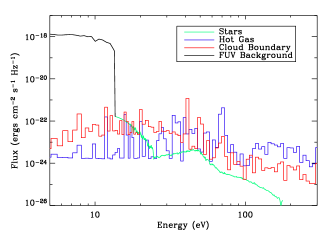
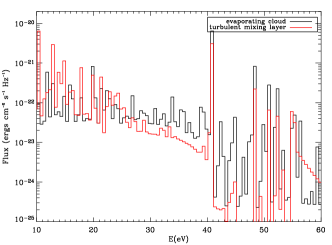
Figure 7: Left: Components of the interstellar radiation incident on the local interstellar cloud complex. Contributions from stars show the EUV flux from nearby white dwarf and B stars, after deabsorbing the corresponding $N$(H^o) to the cloud surface. The cloud boundary flux produced by emission from an evaporative interface between the local gas and the hot gas of the Local Bubble is shown ([Slavin and Frisch, 2002]). Right: Radiation field from a turbulent mixing layer interface compared to that of a conductive interface. Instabilities at the boundaries of tenuous clouds may lead to quite different radiation fields inside of the clouds, particularly near 584 Å where He^o is ionized.

4.2 Radiative Transfer Models of the Local Cloud and other Tenuous ISM

Our radiative transfer models are constrained by observations of local ISM towards nearby stars, and in situ data from LIC neutrals that have penetrated the heliosphere. The in situ data includes direct detection of He^o, observations of solar L${\alpha}$ florescence from H^o in the heliosphere, and observations of the pickup ion and anomalous cosmic ray populations that are seeded by interstellar neutrals (see Moebius et al., Chapter 8). Generally elements with FIP$<$13.6 eV are fully ionized in tenuous clouds, while elements such as H, O, N, Ar, He, and Ne with 13.6  $\buildrel<\over{\sim}$  FIP  $\buildrel<\over{\sim}$  25 eV are partially ionized. Neutrals from these partially ionized species enter the heliosphere, where they seed the pickup ion and anomalous cosmic ray populations measured by instruments on various spacecraft. Column densities towards nearby stars constrain sight-line integrated values, and permit the recovery of $n({\rm H^{+}})$/$n$(H^o) as a function of distance to the cloud surface (Fig. 9). While the LIC temperature is determined directly from Ulysses observations of He^o, the densities $n$(H^o) and $n({\rm H^{+}})$ at the solar location vary as the Sun moves through the LIC, and must be determined from radiative models.

The detailed attention paid here to LIC radiative transfer models is motivated by the facts that $n$(H^o) and $n$(He^o) at the solar location are important boundary conditions of the heliosphere, and that ionization gradients in the CLIC are factors in reconstructing the 3D cloud morphology from data. An extensive study of the LIC ionization has resulted in a series of $\sim$50 radiative transfer models appropriate for tenuous ISM such as the LIC and CLIC ([Slavin and Frisch, 2002, Frisch and Slavin, 2003, Frisch and Slavin, 2005]). These models use the CLOUDY code ([Ferland et al., 1998]), an interstellar radiation field based on known sources, and models for the interface expected between the LIC and Local Bubble plasma (also see §2.2). Boundary conditions for outer scales are provided by ISM data integrated over the LIC, which can be subject to ionization gradients. On inner scales the boundary conditions are given by in situ observations of ISM at the heliosphere. Both sets of constraints are important for evaluating the RT properties of the surrounding ISM where large H^o/${\rm H^{+}}$ gradients are found. The data sets used here include $n$(He^o), pickup ions, and anomalous cosmic rays inside of the heliosphere, and absorption line data of the LIC towards the downwind star $\epsilon$ CMa (GJ, FS).

These RT models will be updated in the future, as the density, composition, LIC magnetic field, radiation field, and interface regions between the LIC and Local Bubble plasma become better understood. The LIC magnetic field enters indirectly through the contribution of magnetic pressure to the cloud interface. The magnetic pressure in the cloud helps to determine the thermal pressure and thus cooling in the interface, so that further studies of $B_{\rm IS}$ near the Sun will provide insight into the characteristics of the interface radiation. One of the significant results of our study is that the spread in predicted neutral and ion densities demonstrates that low column density ISM can be in equilibrium at a range of ionization levels, and that the ionization itself is highly sensitive to the radiation field, interface characteristics, and other cloud properties.

Figure 8: Variation of neutral densities between the Sun and cloud surface for Model 2 from Slavin and Frisch (2002). Shown are variations in neutral column densities between the Sun ($N$(H^o)=6.5$\times$ 10¹⁷ cm^-2) and cloud surface ($N$(H^o)=0) for H^o, He^o, Ne^o, O^o, and N^o. At the heliopause, $n$(He^o)$\sim$0.015 cm^-3, $n$(H^o)$\sim$0.22 cm^-3, $n{\rm(e)}$$\sim$0.1 cm^-3.

4.3 Results of Radiative Transfer Models

Two generations of radiative transfer (RT) models have been developed, with the focus on matching data for the LIC inside of the heliosphere, and matching data on nearby ISM in the downwind direction where the brightest point sources of EUV radiation ($\epsilon$ CMa and $\beta$ CMa) and low column densities are found. Both sets of models are constrained by LIC data obtained inside of the heliosphere, such as for pickup ions, He^o, and anomalous cosmic rays. The PUI and ACR populations are seeded by neutral ISM flowing into the heliosphere, and are subject to filtration losses in the heliosheath regions (Moebius et al., Zank et al., this volume).

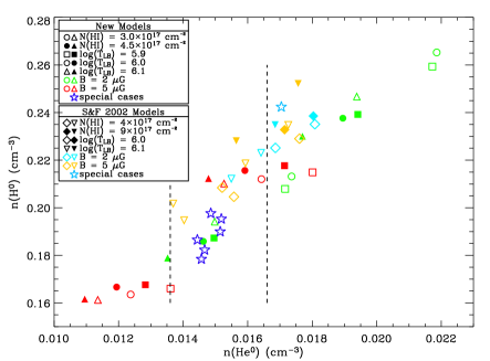
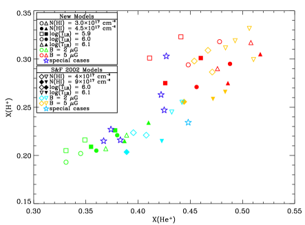
Figure 9: Top: H neutral density vs. He neutral density, both at the Solar location for a large set of model calculations. The symbol colors indicate the assumed magnetic field strength in the cloud, the fill indicates the assumed HI column density, and the shape indicates the assumed temperature of the hot gas of the Local Bubble. Stars represent special parameter sets which do not fall on the grid of model parameters, but rather are chosen to better match the data. The density and uncertainties of He^o are plotted as vertical lines [Möbius et al., 2004]. Note that a range of n(HI) values are consistent with the n(He^o) measurements. The radiative transfer models that provide the best agreement with all available data on the ISM also yield a consistent estimate of $n$(H^o)$=0.19-0.21$ cm^-3. Bottom: Same as left plot but for the ${\rm H^{+}}$ and He⁺ ion fractions. Note: Some of the differences not explained for by $N($H^o$)$, $T_{\mathrm{LB}}$, or $B$ are due to differences in the assumed total H densities.

The ionization state of the pristine ISM outside of the heliosphere is obtained from the RT models, using slightly different constraints for the first and second generations of models. The first generation of 25 models are constrained by the local ISM towards $\epsilon$ CMa, i.e. the sum of the LIC and blue shifted (BC) clouds, and by ISM byproducts inside the heliosphere. The ISM within $\sim$1–2 pc towards $\epsilon$ CMa is divided between two clouds, with projected HC velocities of 10 km s^-1 (the BC) and 18 km s^-1 (the LIC), and with a total $N$(H^o)$<10^{18}$ cm^-2. The LIC and BC are also observed towards Sirius ($\alpha$ CMa, 2.7 pc). Two models, Model 2 and Model 8, provide a good match to all data except for the cloud temperature inside of the heliosphere. The predicted temperature at the heliosphere is $\sim$3,000 K higher than found from in situ He^o data, $T$= 6,400$\pm$340 K. A possible explanation for this difference is that the abundances of coolants such as ${\rm C^{+}}$ are incorrect in the models, particularly since $N$(${\rm C^{+}}$) generally has large measurement uncertainties. A second mismatch occurs because predicted $N$(Si⁺²) values are lower than observed values, which suggests that interface models require additional processes such as a turbulent mixing layer. Models 2 and 8 predict that $n$(H^o)$\sim$0.20 cm^-3, $n{\rm(e)}$$\sim$0.1 cm^-3, and ionizations of $\chi$(H)$\sim$0.30, and $\chi$(He)$\sim$0.49 are appropriate for the solar location ([Slavin and Frisch, 2002, Frisch and Slavin, 2003]). The mean cloud density to the downwind surface is $\langle n$(H^∘)$\rangle_{\mathrm{LIC}}$$\sim$0.17 cm^-3.

The second set of models is constrained by data on the LIC towards $\epsilon$ CMa (excluding the BC) and in situ ISM. The best of these models are in good agreement with the in situ data, including cloud temperature data. However, these models require a high C abundance, possibly in conflict with solar abundances, and fail to predict $N$(Mg⁺)/$N$(Mg^o) in the LIC. The second set of models require that the LIC and BC have different ionization levels, which is similar to the findings of Gry and Jenkins (2001) but remains unexplained. LIC properties predicted by these models, which are still under study, are $n$(H^o)=0.19 cm^-3, $\chi$(H)=0.22, $n{\rm(e)}$=0.06 cm^-3, $n$(He^o)=0.015 cm^-3, and $\chi$(He)=0.37

The results of the RT models that are significant for heliosphere studies are summarized in Figures 8 and 9. The ionizations of H, He, O, N, and Ne throughout the LIC are shown in Fig. 8, with variations of $\sim$25% between the cloud surface and the Sun. Fig. 9 shows the extent of ionization states possible under equilibrium conditions in tenuous ISM. Minor variations in the physical assumptions input to the RT models result in a continuum of ionization levels that are in equilibrium for low density clouds like the LIC. Depending on the RT model constraints, H ionization levels are 0.19–0.23, while He ionization levels are 0.32–0.53. These models show that ionization levels might vary between clouds in the CLIC, so that variations in the heliosphere boundary conditions are expected as the CLIC flows past the Sun (see §3).

5 Passages through Nearby Clouds

The transition of the Sun from the near void of the Local Bubble, and into the stream of tenuous ISM flowing away from the Scorpius-Ophiuchus Association, can be probed with the kinematics and column densities of nearby clouds, combined with models of the volume density $n$(H^o). Specifically, cloud dimensions are assumed to be $\propto$$N$(H^o)/$\langle n$(H^∘)$\rangle$. Radiative transfer models of tenuous ISM show that cloud ionization, $\chi$(H), varies with column density. Since the densities of individual cloudlets are not currently available, $n$(H^o) determined by LIC radiative transfer models is extrapolated to other nearby clouds (§4). With this simple approach, we see that the Sun appears to have entered the CLIC within the past $\sim$140,000 years. The Sun is located close to the downwind edge of the CLIC ([Frisch, 1995]). CLIC physical properties are discussed in §3.

The most predictable passage of the Sun into an interstellar cloud is the epoch at which the Sun entered the LIC, the cloud now surrounding the Sun. The LIC is the only cloud with an accurate 3D velocity vector, which is found from Ulysses measurements of interstellar He^o inside of the solar system. The LIC HC velocity is 26.3$\pm$0.4 km s^-1, and the downwind direction is $\lambda=74.7\pm 0.5$^∘, $\beta$=–5.2$\pm$0.2^∘ (ecliptic coordinates, [Witte, 2004]). Several estimates are given for the epoch of the Sun’s entry into the LIC. Both the data and radiative transfer models, upon which the estimate relies, need further refinement before answers are conclusive. We test several models of the poorly known LIC shape. The observed cloud velocity and the projected LIC velocity towards the $\chi^{1}$ Ori, 8.7 pc away and $\sim$15^∘ from the downwind direction, differ by $\sim$2.4 km s^-1, suggesting non-LIC gas is contributing (Table 4).

The distance to the cloud edge is given by $N$(H^o)/$\langle n$(H^∘)$\rangle$, where $\langle n$(H^∘)$\rangle$ is the average space density of H^o in the cloud. The density of the LIC at the solar location is $n$(H^o)$\sim$0.2 cm^-3, and a mean density $\langle n$(H^∘)$\rangle_{\mathrm{LIC}}$$\sim 0.17$ cm^-3 is found from radiative transfer models of the LIC in the downwind direction (§4). When the cloud structure is not fully resolved, or several velocity components are present, there may be gaps in the cloud that are not incorporated into the adopted value for $\langle n$(H^∘)$\rangle$. We present several estimates below for the entry of the Sun into the LIC, with results that differ by factors of three. However, the answers are consistent with the Sun’s entry into the LIC sometime within the past $\sim$47,000 years for $\langle n$(H^∘)$\rangle$=0.17 cm^-3, and possibly quite recently within the past thousand years.

The difference between the LIC and upwind gas velocities, of $\ {\raise-2.15277pt\hbox{$\buildrel<\over{\sim}$}}\ 2$ km s^-1, including towards the nearest star $\alpha$ Cen, suggest that the properties of the cloud surrounding the Sun will change rather soon, in $\sim$3,800 years.

5.1 First Encounter of Sun with the Local ISM

The projected LIC velocity and $N$(H^o) towards nearby stars in the downwind direction (Table 4), indicates that the Sun entered the CLIC sometime within the past 44,000–140,000/$n_{HI,0.2}$ years, where $n_{HI,0.2}$ is the average cloud density in units of 0.2 cm^-3 (§4, Fig. 9). The value $n_{HI,0.2}$$\sim$1 is reasonable for nearby tenuous ISM, and is consistent with radiative transfer models of the LIC. This transition of the Sun out of the deep vacuum of the Local Bubble, and into the higher density CLIC ISM, would have been accompanied by the appearance of neutral interstellar gas, pickup ions, anomalous cosmic rays, and dust in the heliosphere. The geological record of cosmic ray radioisotopes should have sampled this transition (see the discussions of cosmic rays and the spallation product radioisotopes in Chapters 9, 10, and 12).

The simplest estimate for the date of entry of the Sun into the CLIC is to ignore non-radial motions for all clouds and look only at the nearby stars in the anti-apex direction. ISM towards the three stars $\alpha$ CMaA, $\alpha$ CMaB, and $\epsilon$ CMa are useful for this estimate, giving $N$(H^o)=5–7$\times 10^{17}$ cm^-2 (based on data and models in [Hebrard et al., 1999, Frisch and Slavin, 2003]). The distance to the cloud edge in the anti-apex direction is $\propto$$n_{HI,0.2}$^-1 pc. The most distant of the two cloudlets seen in these sightlines is a blue-shifted cloud, with a heliocentric radial velocity of 9.2–13.7 km s^-1 (Table 1). We then find that the Sun entered the CLIC within the past (59,000–120,000)/$n_{HI,0.2}$ years.

Using instead the ISM towards the stars $\chi^{1}$ Ori and $\alpha$ Aur, which are near the heliocentric downwind direction, and for a distance to the cloud edge given by $N$(H^o)/$n_{HI,0.2}$, the observed radial velocities (Table 4) indicate that the Sun entered the CLIC (44,000–140,000)/$n_{HI,0.2}$ years ago.

For these estimates, possible non-radial cloud motions and gaps between clouds are ignored. The cloud gas filling factor in the downwind direction is $f$$\sim$0.26 in §3. If the downwind CLIC consists of a series of wispy clouds with similar velocities, then $n_{HI,0.2}$$\ll$0.2 cm^-3, and the first solar encounter with the CLIC could have occurred up to $4\times 10^{5}$ years ago based on the $\chi^{1}$ Ori data.

5.2 Entering the Local Cloud

In principle the entry date of the Sun into the surrounding cloud, LIC, can be determined precisely since the full 3D velocity of the LIC is known from observations of He^o inside of the heliosphere (Table 1). The LIC shape is uncertain because components at the LIC velocity are not resolved in many sightlines. Although there may be high density contrasts from low speed waves in the LIC, for instance acoustic waves will have velocities $\sim$7 km s^-1, we take the approach that local clouds are defined by the component structure and look at several geometric LIC models to estimate the epoch the Sun entered the LIC. ISM data for downwind stars are summarized in Table 4.

The simplest estimate (A) uses $N$(H^o) and the LIC velocity towards $\chi^{1}$ Ori, $\sim$15^∘ from the downwind LIC direction. Estimate (B) is based on the closest observed star in the downwind direction, $\alpha$ CMa, which is $\sim$45^∘ from the downwind direction, combined with the assumption that the normal to the downwind cloud surface is parallel to the LSR LIC velocity. This assumption results in an entry epoch that varies with the assumed LSR (§1.2), and ignores data for more distant downwind stars. Estimate (C) approximates the downwind LIC surface as a flat plane, defined by the distance of the LIC edge towards any three stars from Table 4, moving through space at the LIC velocity. The final estimate (D) relies on the Colorado LIC model (RL0), which however does not incorporate the most recent data for the LIC, but can be expected to substantially improve in the future.

A. The values for the LIC $N$(H^o) and the projected LIC velocity towards $\chi^{1}$ Ori (Table 4) indicate that the Sun entered the LIC $\sim$40,000/$n_{HI,0.2}$ years ago, where $n_{HI,0.2}$ is the mean $n$(H^o) to cloud surface in units of 0.2 cm^-3. Radiative transfer models indicate $n_{HI,0.2}$$\sim$0.85 (§4). The observed cloud velocity towards $\chi^{1}$ Ori differs from the projected LIC velocity by 2.4$\pm$1.0 km s^-1, so that additional cloud gas is present in this sightline that is not at the LIC velocity. In addition, the turbulent contribution to the line broadening is $\xi=2.38^{+0.15}_{-0.17}$ km s^-1 towards $\chi^{1}$ Ori (§1.3, [Redfield and Linsky, 2004b]), indicating unresolved cloudlets may be present.

B. For this estimate we use LIC data towards the nearest star in the downwind direction for which ISM data are available, $\alpha$ CMaAB (Sirius). The LIC downwind surface is assumed to be oriented such that the surface normal is parallel to the LIC LSR velocity, based on the model of Frisch (1994, Figure 10). Note that the “downwind” nomenclature is referenced with respect to the Sun, and the “downwind surface” is the leading edge of the LIC as it moves through the LSR. Since the LIC surface is referenced to the LSR, the solar apex motion is a variable (Table 1, §1.2). The Sun then encountered the LIC within the past $\sim$13,500/$n_{HI,0.2}$ years or $\sim 10^{3}$/$n_{HI,0.2}$ years, for the Hipparcos or Standard solar apex motions, respectively. The present distance to the LIC downwind surface is $\sim 0.01-0.3$ pc for this model. The velocity of most of the interstellar gas observed towards $\chi$ Ori and $\alpha$ Aur differs by a small amount, 0.7–1.4 km s^-1, from the projected LIC velocity (Table 4), and therefore is located in a separate cloud. Because the LIC also extends less than $\sim 10^{4}$ AU in the upwind direction, this model implies that the LIC is filamentary or sheet-like, similar to global low density ISM (§6). This model results in an interstellar magnetic field direction, $B_{\rm IS}$, which is approximately parallel to the cloud surface (perpendicular to the surface normal).

Figure 10: SEE fig6.pdf. The distribution of nearby ISM is shown based on the assumption that the LSR motion of the LIC is parallel to the normal of the cloud surface (model B, §5.2). The Sun and LIC motions are in the LSR. Figure from Frisch (2000), courtesy of American Scientist.

Table 4: Stars Sampling the Downwind LIC

Object	$\ell$, $b$	Dist.	Vobserved	V${}^{proj}_{\rm LIC}$	log$N$(Ho)
	(∘, ∘)	(pc)	(km s-1)	(km s-1)	(cm-3)
$\alpha$ Aur	162.6, 4.6	12.9	21.5$\pm$0.5	23.0$\pm$0.3	18.26
LIC Heo	183.3, –15.9	0	26.3$\pm$0.3	26.3$\pm$0.3	–
$\chi^{1}$ Ori	188.5, –2.7	8.7	23.1$\pm$0.7	25.5$\pm$0.3	17.80
$\alpha$ CMi	213.7, 13.0	3.5	20.5$\pm$1.0, 24.0	19.6$\pm$0.2	17.90
$\alpha$ CMaA	227.2, –8.9	2.7	13.7, 19.5$\pm$0.3	19.1$\pm$0.2	17.25
$\alpha$ CMaB	227.2, –8.9	2.7	11.7, 17.6$\pm$1.5	19.1$\pm$0.2	17.63
$\epsilon$ CMa	239.8, –11.3	132	9.2, 16.2$\pm$1.5	15.1$\pm$0.2	$\sim$17.54

Notes: The LIC velocity component is in $italics$. V${}^{proj}_{\rm LIC}$ is the LIC velocity projected towards the star. All velocities are heliocentric. The column densities and data are from Witte (2004), Hebrard et al. (1999), Frisch & Welty (2005), RL, GJ, SF02, and FS.

C. The third estimate models the downwind cloud surface as a locally flat surface moving with the LIC velocity, based on the model in Mueller et al. (2005). We then use any three stars in Table 4 to define this plane, and the time at which the Sun crosses this plane marks the entry of the Sun into the LIC. For this model, the Sun entered the LIC between 33,000/$n_{HI,0.2}$ to 36,000/$n_{HI,0.2}$ years ago.

D. The final estimate relies on the Colorado LIC model, based on density $\langle n$(H^∘)$\rangle$=0.1 cm^-3 and a LIC velocity determined from UV absorption lines towards nearby downwind stars (RL). This UV LIC vector differs by $\sim$0.6 km s^-1 in velocity, and $\sim$0.8^∘ in direction, from the LIC velocity given by data on interstellar He^o inside of the solar system ([Witte, 2004]). The Colorado Model Web calculator gives a distance to the downwind surface of 4.5 pc, indicating the Sun entered the LIC $\sim$170,000 years ago for a relative Sun-LIC velocity of 26.3 km s^-1, or alternatively $\sim$85,500/$n_{HI,0.2}$ years ago. The column density towards the downwind direction is predicted to be $N$(H^o)=$10^{18.14}$ cm^-2, however, which differs substantially from recent values for $\chi^{1}$ Ori (Table 4). We therefore disregard this estimate, but expect further improvements in the Colorado model to significantly increase our understanding of the LIC morphology.

5.3 Future Cloud Encounters

The best limits on the distance to the upwind edge of the LIC are found from observations of 36 Oph, 6 pc away and $\sim 16$^∘ from the heliosphere nose. The ISM velocity towards 36 Oph is –28.5$\pm$0.6 km s^-1, which corresponds to the G-cloud velocity (Table 3). The limit on $N$(H^o) at the projected LIC velocity of 25.7 km s^-1 is $N$(H^o)$<6\times 10^{16}$ cm^-2 ([Wood et al., 2000b]). These numbers indicate that the Sun will exit the LIC sometime within the next $\sim$3700/$n_{HI,0.2}$ years, and that the distance to the upwind LIC surface is $<$0.10 pc. Support for this result is provided by the ISM velocity towards the nearest star $\alpha$ Cen, which is $\sim$50^∘ from the HC nose direction. Towards $\alpha$ Cen, the observed cloud velocity and the projected LIC velocity differ by $\sim$1 km s^-1 ([Landsman et al., 1984, Linsky and Wood, 1996]). Column densities of $N$(H^o)=17.6–18.0 cm^-2 were originally found towards $\alpha$ CenAB ([Linsky and Wood, 1996]), which indicate that $\langle n$(H^∘)$\rangle$ may be similar to the LIC density of $\sim$0.2 cm^-3. Later interpretations of the data favor the low end of this column density range ([Wood et al., 2005]), indicating that the sightline is only partially filled with warm gas.

Possibilities for the next cloud to be encountered by the Sun include the G and Apex clouds (Table 3, [Frisch, 2003]). Both clouds have LSR upwind directions, ($\ell$, $b$)=(348$\pm$3^∘, 5$\pm$5^∘), that are approximately perpendicular to the LSR solar apex motion (§1.2). Observations of $\alpha$ Cen and $\alpha$ Aql show that the G-cloud is within 1.3 pc, and the Apex cloud is within 5 pc of the Sun, giving upper limits for an encounter date of $\sim$45,000 and $\sim$175,000 years, respectively. The column densities of the G-cloud are $\sim$3 times larger than Apex cloud column densities, which are $N$(H^o)$\sim 10^{17.47}$ cm^-2 towards 70 Oph and $\alpha$ Aql. Typical G-cloud column densities are $N$(H^o)$\sim 10^{17.92}$ cm^-2.

Both clouds are inhomogeneous. Only the Apex cloud is seen towards AU Mic (d=9.9 pc, $\ell$=12.7^∘, $b$=–36.8^∘). Only the G-cloud is seen towards $o$ Ser (d=13 pc, $\ell$=13.3^∘, $b$=9.2^∘) and $\nu$ Ser (d=59 pc, $\ell$=10.6^∘, $b$=13.5^∘). Both clouds are seen towards $\alpha$ Aql (d=5 pc, $\ell$=47.7^∘, $b$=–8.9^∘) and $\alpha$ Oph (d=14 pc, $\ell$=35.9^∘, $b$=22.6^∘).

The G-cloud Ca⁺ component ($N$(Ca⁺)=1.58$\times 10^{11}$ cm^-2) towards $\alpha$ Oph is extraordinarily strong for a nearby star, and it implies a density of $n$(H^o)$>$5 cm^-3 in the G-cloud, which is $\sim$15 times the density of the LIC ([Frisch, 2003]). This estimate is found by using the G-cloud limit of $N$(Ca⁺)/$N$(H^o)$<7.1\times 10^{-9}$ towards $\alpha$ Cen in order to estimate $N$(H^o) for the G-cloud in the $\alpha$ Oph sightline, and by assuming the G-cloud is entirely foreground to $\alpha$ Cen, giving a distance limit of 1.3 pc. However, should the G-cloud temperature be colder towards $\alpha$ Oph than towards $\alpha$ Cen, or should a significant amount of the G-cloud be beyond the distances of 36 Oph and $\alpha$ Cen, then the requirement for a high density becomes diminished.

6 The Solar Environment and Global ISM

The global properties of ISM in the solar neighborhood offer hints about potential variations in the ISM that might impact the heliosphere.

Over the past $\sim$50 years, radio and UV data have slowly disproved simple ISM models consisting of gravitationally clumped clouds embedded in a substrate of warm or hot low density gas. Evidence supporting a filamentary nature for low column density ISM, with $N$(H)$<10^{21}$ cm^-2, is provided by H^o 21 cm observations of high latitude H^o filaments, and also by UV observations that are interpreted as high space density ($n$(H^o)$>$10 cm^-3), low column density ( $N$(H^o)$<10^{19}$ cm^-2 and $N({\rm H^{+}})$$<10^{18}$ cm^-2) nearby gas ([Hartmann and Burton, 1997, Welty et al., 1999, Welty et al., 2002]). Towards 23 Ori, warm low velocity diffuse gas has densities in the range $n$(H^o)=15–20 cm^-3, and cloud thicknesses, $L$, are 0.7–0.9 pc. The densities of cold clouds, with temperatures $\leq$100 K, are slightly lower, $n$(H^o)=10–15 cm^-3. Diffuse ionized gas is present at intermediate velocities, $|V_{\rm LSR}|\geq 20$ km s^-1, $n{\rm(e)}$$\leq$5 cm^-3, and $L$= 0.0006–0.04 pc. Thin diffuse ionized clouds, with $n{\rm(e)}$$\sim$0.17 cm^-3, $L$= 0.2–2.7 pc, and similar velocities, are observed towards Orion stars spread over $>$15^∘, which indicates that these clouds must be thin sheets or filaments.

Winds of massive stars and supernova in young stellar associations eject energy into the surrounding ISM, and evacuate cavities in the ISM that are surrounded by irregular shells of WNM. These shells, which may overlap or be filled with X-ray plasma, are traced by H^o 21-cm emission, and explain some of the ISM filamentary structure ([MacLow and McCray, 1988, Cox and Smith, 1974, Dickey, 2004, Heiles and Troland, 2003b]). The CLIC appears to be a fragment of a superbubble shell from one epoch of star formation in the SCA, and $\alpha$ Oph may be in a direction that is tangential to this shell ([Frisch, 1995]).

6.1 Warm Ionized and Partially Ionized Gas

Interstellar plasma and neutrals interact with the heliosphere in fundamentally different ways, and small variations in the interstellar radiation field convert neutral gas to plasma. Nearby WPIM was discussed in §3.1, and we now compare warm interstellar plasma over 100 pc scales and show that the CLIC and global observed diffuse ionized gas are similar. We conclude that dense ionized ISM has not been, and will not be, part of the immediate solar environment over short timescales. However, diffuse WPIM similar to the LIC and CLIC is much more widespread.

Dense fully ionized ISM is not found close to the Sun, although diffuse ionized gas surrounds many hot stars at distances of $>$150 pc, such as $\beta$ CMa bordering the giant ionized Gum Nebula, $\beta$ Cen, which energizes the interior of Loop I, and several stars in Upper Scorpius. Generally H II regions surround hot O, early B, and white dwarf stars that emit strongly in the EUV, $\lambda<$912 Å. The solar path is unlikely to traverse an H II region surrounding an O–B1 star over timescales of $\pm$4 Myrs because there are no hot stars or dense H II regions nearby. The closest H II region surrounds the high latitude star $\alpha$ Vir, 80 pc away. White dwarf stars are relatively frequent near the Sun. Over 25 white dwarf stars with surface temperatures $T>10^{4}$ K are found within 20 pc, and $>40$% of these stars are hotter than 15,000 K. Small Stromgren spheres will surround the hottest white dwarf stars, but the densities will be very low for nearby stars ([Tat and Terzian, 1999]).

Diffuse ionized gas is widespread, in contrast to dense ionized gas. It is traced by weak optical recombination lines such as the H$\alpha$ line, N ii, He i, He ii, O i, and Si ii ([Haffner et al., 2003],[Reynolds, 2004]), UV absorption lines ([Welty et al., 1999, Holberg et al., 1999, Lehner et al., 2003], GJ), and EUV observations of He^o and He⁺ towards white dwarf stars (§3). Pulsar dispersion measures trace the interactions between pulsar wave packets and electrons (e.g. [Taylor and Cordes, 1993, Cordes and Lazio, 2002, Armstrong et al., 1995]). These data reveal a low density, ionized component, $n{\rm(e)}$$\sim$0.1 cm^-3, which fills $\sim$20% of the volume of a 2-kpc-thick layer around the Galactic disk. The diffuse ${\rm H^{+}}$ has been mapped in the northern hemisphere by WHAM, however the LIC emission measure is an order of magnitude below the WHAM sensitivity (e.g. [Reynolds, 2004]). About 30% of diffuse H^o and ${\rm H^{+}}$ gas are found in spatially and kinematically associated clouds with densities $\sim$0.2–0.3 cm^-3 ([Reynolds et al., 1995]). If the H^o and ${\rm H^{+}}$ were spatially coincident in these clouds then $\chi$(H) would be $\sim 0.4$, but Reynolds et al. argue that the H^o and ${\rm H^{+}}$ are spatially separated. Despite the evidence from spatial maps and line widths, however, we believe that the existence of some true WPIM (perhaps at lower ionization levels) cannot be ruled out in these regions. These clouds are associated with large filamentary or sheet-like structures, and exhibit cloud densities and hydrogen ionization levels that are similar to LIC values. In other directions, H${\alpha}$ line emission indicates that H is highly ionized in the WIM, $\chi$(H)$\sim$1. Emission at 588 Å from He^o shows that for the WIM $\chi$(He)$\sim$0.3–0.6. Ratios of $\chi$(He)/$\chi$(H) are $\sim$0.3–0.6 are found, versus $\sim$1.6 for the LIC, implying that the LIC radiation field is harder than for most of the WIM, perhaps because of lower column densities. The WIM has a continuum of temperatures, 5000–10,000 K, and ionization levels, as demonstrated by emission in [N ii], [O i], and [S ii] lines that trace temperature and ionization.

The interstellar plasma is structured over all spatial scales, and these plasma clumps appear to be similar to the LIC. The plasma is partially opaque to radio emission in the energy range 0.1 to 10 MHz, and as a result synchrotron emission probes the WIM clumpiness ([Kulkarni and Heiles, 1988, Peterson and Webber, 2002]). Models for the propagation of low frequency synchrotron emission through a clumpy WIM fit the radio data better than do propagation models, that assume a uniformly distributed parallel slab model for the WIM. These clumps have density $n{\rm(e)}$$\sim$0.2 cm^-3, fill 8%–15% of the disk, and have a free-free opacity at 10 MHz that is consistent with WIM temperatures as low as 4500 K. The dispersion, refraction and scintillation of pulsar wave packets indicates that the WIM is turbulent over scale sizes $10^{-2}-10^{2}$ AU, or even larger, $\sim 10^{2}$ pc, if Faraday rotation and plasma density gradients are included ([Armstrong et al., 1995]).

The WIM properties are consistent with predictions of the radiative transfer models, which find $\chi$(${\rm H^{+}}$)=0.15–0.35, $T\sim 5,000-9,000$ K, and $n$(H^o)=0.2–0.3 cm^-3 for low column density clouds (Fig. 9, [Slavin and Frisch, 2002]). For very low column densities, $<$10¹⁸ cm^-2, a continuum of ionization and temperature levels are expected from variations in the cloud column density and the EUV radiation field. The WNM and WIM in the CLIC may show similar variations, if the $N$(H^o)$\sim$10¹⁹ cm^-2 clouds represent clusters of lower column density objects. The uncertain role of turbulence in cloud evolution allow this possibility.

6.2 Neutral Interstellar Gas and Turbulence

Radio and UV observations of low $N$(H^o) cloudlets in the solar vicinity indicate that dense, low column density, cloudlets may be hidden in the CLIC flow. Radio 21-cm data indicate ISM of this type is widespread, and has column densities and kinematics similar to CLIC ISM.

Two populations of interstellar clouds, WNM and CNM, are found based on observations of the collisionally populated H i hyperfine 21-cm line towards radio-continuum sources. The recent Arecibo Millennium Survey used an ON-OFF observing strategy to survey the properties of H^o clouds towards $\sim$80 radio continuum sources, including emission and and opacity profiles, which were then fit with $\sim$375 Gaussian components. The detailed attention paid to sources of noise and line contamination yielded a data set that provides a new perspective on the statistics of low $N$(H^o) CNM and WNM clouds ([Heiles and Troland, 2003a, Heiles and Troland, 2003b]).

The CNM and WNM components observed in the Arecibo survey show that $\sim$25% of the ISM H^o mass is contained in clouds traveling with velocities $\geq$10 km s^-1 through the local standard of rest. When the solar apex motion of 13–20 km s^-1 is included, this means that Sun-cloud encounters with relative velocities larger than 25 km s^-1 are quite likely, as we might have guessed because of the LIC heliocentric velocity of –26.3 km s^-1.

For 21-cm absorption components with spin temperature $T_{\rm s}$, the opacity is $\tau\propto$$N$(H^o)/$T_{\rm s}$ and the line width is FWHM$\propto$$\sigma$_v, where $\sigma$_v is the dispersion in cloud velocity. Therefore the turbulent ($\Delta V_{\rm turb}$) and thermal contributions to $\sigma$_v can be distinguished for the CNM. Spin temperatures, $T_{\rm s}$, for the CNM are typically $\sim$20–100 K.

The Arecibo survey discovered that 60% of the diffuse ISM is WNM, and $\sim$40% is CNM. Median column densities for the WNM and CNM towards sources with $|$$b$$|>$10^∘ are $N$(H^o)=1.3 $\times$ 10¹⁹ cm^-3 and 5.2 $\times$ 10¹⁹ cm^-3, respectively. The finding that CNM column densities are typically lower than WNM values was unexpected. The column density weighted median spin temperature for the CNM is 70 K, although minimum temperatures are 20 K or lower. Upper limits on WNM kinetic temperatures are 15,000 K or higher, with a typical value of 4,000 K. The turbulent velocities derived for CNM components indicate that the turbulence must be highly supersonic, with a turbulent Mach number $M_{\rm turb}=3\Delta V_{\rm turb}^{2}/C^{2}_{\rm s}\sim$3, where $C^{2}_{\rm s}$ is the sound speed and the factor of 3 converts to three-dimensional turbulence ([Heiles, 2004b]). The densities of the CNM observed towards 23 Ori are $>$10 cm^-3 ([Welty et al., 1999]).

The velocities of CLIC, WNM, and CNM components are compared in Fig. 11. Only high latitude WNM and CNM data with $|$$b$$|>$25^∘ are included, in order to avoid distant gas near the galactic plane. Some of the CNM and WHM components are found at velocities lower than –25 km s^-1, which may be partly due to infalling H^o gas at high latitudes. Otherwise, the CLIC kinematics and column densities overlap generic WNM and CNM values.

Figure 11: SEE figures fig11a.pdf and fig11b.pdf. Left: CLIC velocities, for d$<$50 pc, are plotted against CNM and WNM velocities for sightlines with $|$$b$$|>$25^∘ in the Arecibo Millennium Survey [Heiles and Troland, 2003b]. The Arecibo clouds are within $\sim$425 pc if the H^o layer thickness is 185 pc. The CLIC $N$(H^o) is based on D^o/H^o$=1.5\times 10^{-5}$, Ca⁺/H^o$=8.3\times 10^{-9}$, or ${\rm Mg^{+}}$/H^o$=6.7\times 10^{-6}$, and LSR_Std is used. Right: This composite profile shows that some CNM components can be lost in the WNM at UV resolutions. The solid line shows a D^o 1215 Å absorption component formed by two clouds at the same velocity (0 km s^-1) and column density ($N$(D^o)$=10^{13.17}$ cm^-2), but different temperatures (50 K and 7,000 K). The dashed line shows WNM only, with $N$(D^o)$=10^{13.17}$ cm^-2 and $T=7000$ K. This theoretical profile incorporates a Gaussian instrument resolution of FWHM 3 km s^-1 appropriate for UV data. Turbulent broadening is not included.

Of special interest are very low column density cold CNM, or “tiny” clouds, found for a broad range of velocities. An example is a component with $T_{\rm s}$=16.6 K, $N$(H^o)=2 $\times$10¹⁸ cm^-2 and velocity $-40.6$ km s^-1 observed towards 3C 225. Another example is a component with $T_{\rm s}$=43 K, $N$(H^o)$=3\times 10^{18}$ cm^-2, and velocity –4.6 km s^-1 observed towards 4C 32.44. In addition, CNM components with $N$(H^o)$\sim$10¹⁸ cm^-3, $T_{\rm s}$$\sim$30–90 K, and velocities –30 to 0 km s^-1, are confirmed towards several other sources ([Stanimirovic and Heiles, 2005, Braun and Kanekar, 2005]).

CNM ISM is detected in the UV towards 23 Ori, with low column densities, weak ionization, and low temperatures: $N$(H)$\ {\raise-2.15277pt\hbox{$\buildrel>\over{\sim}$}}\ 2$ x $10^{19}$ cm^-2, $T_{\rm s}$$\sim$60–150 K, and $\sim$1% ionization. Cold clouds with lower column densities may be difficult to resolve at UV resolutions. The densities of these clouds are found from pressure considerations using C i and C ii fine structure lines ([Jenkins, 2002]), and yield $n_{\rm H}$$\sim$10-15 cm^-3 and a cloud thickness of $\sim$0.5 pc ([Welty et al., 1999]). These components are formed in the Orion-Eridanus Bubble shell. Similar features are observed in other Orion stars. This CNM is either filamentary or sheet-like, and it is a plausible template for the CNM in Fig. 11.

The evident crowding of absorption components in velocity space may introduce problems with the interpretation of UV data (§1.3). CNM and WNM clouds with low $N$(H^o) and similar velocities would be unresolved at a nominal 3 km s^-1 UV resolution, as shown by the theoretical composite D^o profile plotted in Fig. 11. This profile is synthesized from the expected profiles of two clouds at 0 km s^-1, temperatures 7,000 K and 50 K clouds, and each with $N$(H^o)=10¹⁸ cm^-2. An instrumental resolution of 3 km s^-1 is included, but turbulence is not. Resolution problems are worse for heavy elements, since the line FWHM$\propto mass^{\rm-1/2}$. Therefore local low $N$(H^o) cold cloudlets can not be ruled out, and if present would be traversed by the heliosphere in $\sim$1–20,000 years.

6.3 Magnetic Fields

Interstellar magnetic fields interact strongly with the heliosphere, and modify the propagation of galactic cosmic rays in space. Unfortunately the uniformity and strength of the interstellar magnetic field ($B_{\rm IS}$) at the Sun are unknown. We showed that magnetic field strengths of $B_{\rm IS}$$\sim$0.6–3.7 $\mu$G would satisfy several assumptions about the equilibrium of local ISM (§3.4). However, the only direct data on the nearby magnetic field are the starlight polarization data attributed to weakly aligned interstellar grains in the nearest $\sim$35 pc ([Tinbergen, 1982, Frisch, 1990]). More recently, it appears as if these grains are instead trapped in the magnetic wall of the heliosheath ([Frisch, 2005]). The global nearby $B_{\rm IS}$ thus must be used to obtain insight on $B_{\rm IS}$ near the Sun.

The properties of the interstellar magnetic field, including the weak spatially uniform ($B_{\rm u}$) and stronger random ($B_{\rm r}$) components, are known for both CNM and WIM (e.g. [Beck, 2001, Crutcher et al., 2003, Heiles, 2004a, Heiles and Crutcher, 2005]). The CNM median field strength of 6.0$\pm$1.8 $\mu$G is determined from data on the Zeeman splitting of the H i 21 cm line ([Heiles and Troland, 2005]), but may not apply to the CLIC where CNM is not yet detected. Although $B_{\rm IS}$$\sim n$ for densities larger than 10³ cm^-3, at lower densities $B_{\rm IS}$ strengths are uncorrelated with cloud density, in violation of simple flux freezing assumptions.

Pulsar data, synchrotron emission, and starlight polarization data indicate that the ratios of the random ($B_{\rm r}$) and uniform ($B_{\rm u}$) components of the local field are $B_{\rm u}$/$B_{\rm r}$$\sim$0.6–1.0. Synchrotron emission of external galaxies indicate that the ratio $B_{\rm u}$/$B_{\rm r}$ increases in interarm regions such as surrounding the Sun, but decreases in spiral arm regions as the magnetic fields become more random. Comparisons of magnetic field strengths determined from polarized synchrotron emission and pulsar dispersion measure observations, which interact with $B_{\rm IS}$ and the WIM, give the total local field strength and the relative strengths of $B_{\rm u}$ and $B_{\rm r}$. Synchrotron emission gives a total field strength locally of $B_{\rm IS}$$\sim 6\pm 2\leavevmode\nobreak\ \mu$G, and the uniform component strength $B_{\rm u}$$\sim 4\leavevmode\nobreak\ \mu$G. Faraday rotation from the propagation of the oppositely polarized circular components produces a polarization phase shift, given by the rotation measure RM =$\int_{0}^{L}B_{\rm||}$(x)$n_{\rm e}(x)dx$, which responds to the parallel component of the magnetic field, $B_{\rm||}$, weighted by the electron density, $n$${}_{\rm e}(x)$, and integrated over pathlength $L$. $B_{\rm IS}$ is directed away from the observer for RM$<$0. Wave packet dispersion in the WIM gives the dispersion measure DM = $\int_{0}^{L}\hbox{$n$}_{\rm e}(x)dx$. The mean local field, weighted by $n{\rm(e)}$, is found from the ratio RM/DM and is $B_{\parallel}$$\sim 6.5\leavevmode\nobreak\ \mu$G, where $B_{\rm u}$$\sim$$B_{\parallel}$.

Starlight polarization data show that the local $B_{\rm IS}$ is relatively uniform, and not strongly strongly distorted or tangled by turbulence. Locally the total field, $B_{\rm IS}$, follows the pitch angle, 9.4^∘, of the local spiral arm, and has a curvature radius of $\sim$7.8 kpc centered on $\ell$=344.6^∘. The starlight polarization vectors converge near $\ell$$\sim$80^∘ and $\sim$270^∘, where the random component of the field, $B_{\rm r}$, results in a polarization angle that is rotated over all angles.

A large excursion from $B_{\rm u}$ is seen towards within 150 pc, towards Loop I, where both polarized starlight and synchrotron emission indicate a magnetic field conforms to the superbubble shell around the Scorpius-Centaurus Association. Surveys of $B_{\parallel}$ in morphologically distinct objects such as the Loop I, Eridanus, and Orion supershells, show that the magnetic field is strong, $B_{\parallel}$$>5\leavevmode\nobreak\ \mu$G, and ordered throughout these shell features.

6.4 Origin of Local ISM

Several origins have been suggested for the CLIC. CLIC kinematics and abundance patterns led to the suggestion that the CLIC is part of a superbubble shell surrounding the Scorpius-Centaurus Association ([Frisch, 1981, Frisch and York, 1986, de Geus, 1992, Frisch, 1995]). The SCA is surrounded by a well-known supershell formed by epochs of star formation, winds from massive stars and supernovae ([Weaver, 1979]). Using superbubble expansion models and the star formation rates in the SCA, Frisch modeled the CLIC as a fragment of the shell from the formation of the Upper Scorpius subgroup ($\sim 4$ Myrs old) of the SCA, which has expanded away from the high-density ISM close to the association to the lower pressure regions around the Sun ([Frisch, 1995]). A related suggestion attributes the origin of the CLIC to Rayleigh-Taylor instabilities in the shell of the younger Loop I supernova remnant ($\sim$0.5 Myrs old), which has propelled ISM towards the Sun ([Breitschwerdt et al., 2000]). A third origin suggests that the CLIC originates as a magnetic flux tube that is originally captured in the inner wall of the Local Bubble surrounding the Sun, and is driven back into the Local Bubble interior by magnetic tension ([Cox and Helenius, 2003]). This scenario requires that the CLIC velocity and magnetic fields are parallel, which appears unlikely because of the asymmetric capture of small interstellar dust grains in the heliosheath ([Frisch, 2005]). Each of these suggestions is consistent with the CLIC kinematics, but should have different consequences for short-term variations in the solar environment.

7 Summary

In this chapter we have tried to present the essential information required to understand short-term variations in the galactic environment of the Sun, and at the same time make an educated guess about the times that the Sun has transitioned between different types of ISM for the past $10^{3}-10^{5}$ years. It is our hope some day that the geological radio isotope records can be searched for the signatures of these transitions, although earlier searches have been inconclusive (e.g., [Frisch, 1981, Sonett et al., 1987, Frisch, 1997]).

Both the Sun and ISM move through our local neighborhood of the Milky Way Galaxy, which is described by the LSR rest velocity frame (with its own uncertainties). The Sun has been in the nearly empty space of the Local Bubble interior for several million years. Sometime in the past $\sim$140,000/$n_{HI,0.2}$ years, the Sun exited the nearly empty Local Bubble and entered an outflow of ISM with an upwind direction towards the Scorpius-Centaurus Association. Even more recently, $\sim$40,000/$n_{HI,0.2}$ years ago, the Sun entered the cloud now surrounding us, the LIC. Within $\sim$4,000 years the Sun will exit the LIC. What’s next? The flow of local ISM past the Sun is bearing down on the Sun at a relative velocity of $\sim$28 km s^-1, the cloudlets in this flow are expected to pass over the Sun more often than roughly once per $\sim$70,000 years. The next cloud the Sun is most likely to traverse is either the G-cloud or the Apex Cloud. This cloud must be either either inhomogeneous or denser by a factor of $\sim$30 than the LIC.

Most of this nearby ISM is warm partially ionized gas, not dissimilar to warm ISM observed elsewhere, except that column densities tend to be lower. The properties of this gas are mainly consistent with predictions of radiative transfer models, which then suggests that the local gas is close to equilibrium. If viewed from elsewhere in the galaxy, the ensemble of ISM close to the Sun could easily pass as warm neutral material such as observed by H i 21 cm data. The general characteristics of nearby ISM are similar to the global warm neutral material, except that column densities are very low so that H^o ionizing photons penetrate to the cloud cores. The physical properties of the CLIC vary both between and within clouds. The low column densities of this ISM lead to ionization variations inside of a cloud. As the Sun passes between clouds, the interstellar ionization, dynamic pressure or the thermal pressure may vary, possibly all at once. As a consequence, the boundary conditions of the heliosphere may experience dramatic variations as the Sun moves through the CLIC. The efforts to understand these variations have just begun.

One of the more intriguing possibilities is that tiny cool ISM cloudlets are undetected in the nearby warm partially ionized gas (WPIM). Such structures, with $N$(H^o)$\sim 10^{18}$ cm^-2, are seen elsewhere, although infrequently. A new class of cloud models, perhaps based on macro-turbulence, will be required if such structures exist locally.

Most of our conclusions have substantial inherent uncertainties. The most prominent is that all distances, such as those to cloud edges, are based on $N$(H^o), which is moderately well known for most sightlines discussed here, and an assumption about the mean H^o space density, $\langle n$(H^∘)$\rangle$. We have a very good idea of the value for $\langle n$(H^∘)$\rangle$ in the LIC because of extensive development of radiative transfer models for the LIC. Our confidence in the models follows from their ability to predict both ISM densities inside of the heliosphere, including the Ulysses satellite values for $n$(He^o), and ISM column densities towards nearby stars. Since column densities are too small locally for measurements of the fine-structure lines that yield $n$(H^o), we have assumed that the LIC value for $\langle n$(H^∘)$\rangle$ applies elsewhere in the CLIC. In addition, the transition epochs for the Sun are calculated by assuming that there are no gaps between individual cloudlets, as defined by velocity. The LIC $\langle n$(H^∘)$\rangle$ value is probably representative of the downwind CLIC, because the Sun is so close to the downwind edge. However, we can not rule out gaps between the cloudlets, and such gaps would alter estimates of the epoch the Sun entered the CLIC.

One of the most significant improvements will be to make good maps of nearby ISM. Such maps would require a new generation of space instrumentation, capable of high resolution, R$\sim$500,000, and high signal-to-noise observations of both bright and faint objects over the spectral range 912–3,000 Å. We also need more precise measurements of the diffuse interstellar radiation field, throughout the full spectral interval of 2000 Å to 0.1 keV. Such data would provide a strong constraint on the interface emission and reduce uncertainties in the ${\rm Mg^{o}}$ photoionization rate.

In this chapter we have reviewed the short-term variations in the galactic environment of the Sun. Our galactic environment affects the heliosphere, and by analogy the astrospheres of nearby stars, so that the space trajectory of a star is a filter for other planetary systems with conditions conducive to stable climates for exoplanets ([Frisch, 1993]). As other papers in this volume demonstrate, the ISM-modulated heliosphere has a pronounced effect on the cosmic ray flux in the inner heliosphere, which in turn appears to affect the climate. Similar processes will affect the climates of planets outside of the solar system. Such possibilities make the study of short-term variations in the galactic environment of the Sun highly topical.

Acknowledgments: The authors thank NASA for supporting this research through grants NAG5-11005, NAG5-13107 and NAG5-13558. This article will appear in the book ”Solar Journey: The Significance of Our Galactic Environment for the Heliosphere and Earth”, Springer, in press (2006), editor P. C. Frisch.

References

- [Adams and Frisch, 1977] Adams, T. F. and Frisch, P. C. (1977). High-resolution observations of Lyman alpha sky background. ApJ, 212:300–308.
- [Adams, 1949] Adams, W. S. (1949). Observations of interstellar H and K, molecular lines, and radial velocities in spectra of 300 O and B stars. ApJ, 109:354–379.
- [Armstrong et al., 1995] Armstrong, J. W., Rickett, B. J., and Spangler, S. R. (1995). Electron density power spectrum in the local interstellar medium. ApJ, 443:209–221.
- [Bash, 1986] Bash, F. (1986). Present, Past and Future Velocity of Nearby Stars: The path of the Sun in 108 Years. In Galaxy and the Solar System, pages 35–46. University of Arizona Press.
- [Beck, 2001] Beck, R. (2001). Galactic and Extragalactic Magnetic Fields. Space Science Reviews, 99:243–260.
- [Bohlin et al., 1978] Bohlin, R. C., Savage, B. D., and Drake, J. F. (1978). A survey of interstellar H I from L-alpha absorption measurements. ApJ, 224:132–142.
- [Braun and Kanekar, 2005] Braun, R. and Kanekar, N. (2005). Tiny H I clouds in the local ISM. A&A, 436:L53–L56.
- [Breitschwerdt et al., 2000] Breitschwerdt, D., Freyberg, M. J., and Egger, R. (2000). Origin of H I clouds in Local Bubble. I. Hydromagnetic Rayleigh-Taylor instability caused by interaction of Loop I and Local Bubble. A&A, 361:303–320.
- [Bruhweiler and Kondo, 1982] Bruhweiler, F. C. and Kondo, Y. (1982). UV spectra of nearby white dwarfs and the nature of the local interstellar medium. ApJ, 259:232–243.
- [Cheng and Bruhweiler, 1990] Cheng, K. and Bruhweiler, F. C. (1990). Ionization processes in local interstellar medium - effects of hot coronal substrate. ApJ, 364:573–581.
- [Cordes and Lazio, 2002] Cordes, J. M. and Lazio, T. J. W. (2002). NE2001.I. A New Model for Galactic Distribution of Free Electrons and its Fluctuations. ArXiv Astrophysics e-prints.
- [Cowie and McKee, 1977] Cowie, L. L. and McKee, C. F. (1977). Evaporation of spherical clouds in a hot gas. I - Classical and saturated mass loss rates. ApJ, 211:135.
- [Cox, 2000] Cox, A. N. (2000). Allen’s Astrophysical Quantities, pages 29–30. AIP Press.
- [Cox, 1998] Cox, D. P. (1998). Modeling the Local Bubble. LNP Vol. 506: IAU Colloq. 166: The Local Bubble and Beyond, 506:121–131.
- [Cox and Helenius, 2003] Cox, D. P. and Helenius, L. (2003). Flux-Tube Dynamics and Model for Origin of Local Fluff. ApJ, 583:205–228.
- [Cox and Smith, 1974] Cox, D. P. and Smith, B. W. (1974). Large-scale effects of supernova remnants on Galaxy: Generation and maintenance of a hot network of tunnels. ApJ, 189:L105–L108.
- [Cravens, 2000] Cravens, T. E. (2000). Heliospheric X-ray Emission Associated with Charge Transfer of Solar Wind with Interstellar Neutrals. ApJ, 532:L153–L156.
- [Cravens et al., 2001] Cravens, T. E., Robertson, I. P., and Snowden, S. L. (2001). Temporal variations of geocoronal and heliospheric X-ray emission associated with solar wind interaction with neutrals. J. Geophys. Res., 106:24883–24892.
- [Crutcher et al., 2003] Crutcher, R., Heiles, C., and Troland, T. (2003). Observations of Interstellar Magnetic Fields. Lecture Notes in Physics, Berlin Springer Verlag, 614:155–181.
- [Crutcher, 1982] Crutcher, R. M. (1982). The local interstellar medium. ApJ, 254:82–87.
- [de Geus, 1992] de Geus, E. J. (1992). Interactions of stars and interstellar matter in Scorpio Centaurus. A&A, 262:258–270.
- [Dehnen and Binney, 1998] Dehnen, W. and Binney, J. J. (1998). Local stellar kinematics from Hipparcos data. MNRAS, 298:387–394.
- [Dickey, 2004] Dickey, J. M. (2004). Is the Local Fluff typical? Adv. Space Res., 34:14–19.
- [Dupuis et al., 1995] Dupuis, J., Vennes, S., Bowyer, S., Pradhan, A. K., and Thejll, P. (1995). Hot White Dwarfs in Local Interstellar Medium: Hydrogen and Helium Interstellar Column Densities and Stellar Effective Temperatures from EUVE Spectroscopy. ApJ, 455:574.
- [Dutra and Bica, 2002] Dutra, C. M. and Bica, E. (2002). A catalogue of dust clouds in the Galaxy. A&A, 383:631–635.
- [Ebel, 2000] Ebel, D. S. (2000). Variations on solar condensation: Sources of interstellar dust nuclei. J. Geophys. Res., 105:10363–10370.
- [Eggen, 1963] Eggen, O. J. (1963). Luminosities, colors, and motions of the brightest A-type stars. AJ, 68:689.
- [Ferland et al., 1998] Ferland, G. J., Korista, K. T., Verner, D. A., Ferguson, J. W., Kingdon, J. B., and Verner, E. M. (1998). Cloudy 90: Numerical simulation of plasmas and their spectra. PASP, 110:761–778.
- [Ferlet et al., 1993] Ferlet, R., Lagrange-Henri, A.-M., Beust, H., Vitry, R., Zimmermann, J.-P., Martin, M., Char, S., Belmahdi, M., Clavier, J.-P., Coupiac, P., Foing, B. H., Sevre, F., and Vidal-Madjar, A. (1993). Beta Pictoris protoplanetary system. XIV - Observations of Ca II H and K lines. A&A, 267:137–144.
- [Fitzgerald, 1968] Fitzgerald, M. P. (1968). Distribution of interstellar reddening material. AJ, 73:983.
- [Florinski et al., 2004] Florinski, V., Pogorelov, N. V., Zank, G. P., Wood, B. E., and Cox, D. P. (2004). On the Possibility of a Strong Magnetic Field in the Local Interstellar Medium. ApJ, 604:700–706.
- [Frisch, 1999] Frisch, P. (1999). Galactic Environments of Sun and Cool Stars, pages 3–10. Editions Frontieres.
- [Frisch and York, 1986] Frisch, P. and York, D. G. (1986). Interstellar clouds near the Sun. In The Galaxy and the Solar System, pages 83–100. University of Arizona Press.
- [Frisch, 1979] Frisch, P. C. (1979). Interstellar Material towards Chi Ophiuchi. I - Optical observations. ApJ, 227:474–482.
- [Frisch, 1981] Frisch, P. C. (1981). The Nearby Interstellar Medium. ”Nature”, 293:377–379.
- [Frisch, 1990] Frisch, P. C. (1990). Characteristics of the local interstellar medium. In Grzedzielski, S. and Page, D. E., Eds., Physics of the Outer Heliosphere, pages 19–22.
- [Frisch, 1993] Frisch, P. C. (1993). G-star astropauses - A test for interstellar pressure. ApJ, 407:198–206.
- [Frisch, 1994] Frisch, P. C. (1994). Morphology and Ionization of Interstellar Cloud Surrounding the Solar System. Science, 265:1423.
- [Frisch, 1995] Frisch, P. C. (1995). Characteristics of Nearby Interstellar Matter. Space Sci. Rev., 72:499–592.
- [Frisch, 1997] Frisch, P. C. (1997). Journey of the Sun. http://xxx.lanl.gov/, page astroph/9705231.
- [Frisch, 2000] Frisch, P. C. (2000). The Galactic Environment of Sun. American Scientist, 88:52–59.
- [Frisch, 2003] Frisch, P. C. (2003). Local Interstellar Matter: The Apex Cloud. ApJ, 593:868–873.
- [Frisch, 2005] Frisch, P. C. (2005). Tentative Identification of Interstellar Dust in the Magnetic Wall of Heliosphere. ApJ, 632:L143–L146.
- [Frisch et al., 1990] Frisch, P. C., Welty, D. E., York, D. G., and Fowler, J. R. (1990). Ionization in nearby interstellar gas. ApJ, 357:514–523.
- [Frisch et al., 1999] Frisch, P. C., Dorschner, J. M., Geiss, J., Greenberg, J. M., Grün, E., Landgraf, M., Hoppe, P., Jones, A. P., Krätschmer, W., Linde, T. J., Morfill, G. E., Reach, W., Slavin, J. D., Svestka, J., Witt, A. N., and Zank, G. P. (1999). Dust in the Local Interstellar Wind. ApJ, 525:492–516.
- [Frisch et al., 2002] Frisch, P. C., Grodnicki, L., and Welty, D. E. (2002). Velocity Distribution of Nearest Interstellar Gas. ApJ, 574:834–846.
- [Frisch et al., 2005] Frisch, P. C., Jenkins, E. B., Johns-Krull, C., Sofia, U. J., Welty, D. E., York, D. G., and Aufdenberg, J. (2005). Local Interstellar Matter towards UMa. in preparation.
- [Frisch et al., 1990] Frisch, P. C., Sembach, K., and York, D. G. (1990). Studies of the local interstellar medium. VIII - Morphology and kinematics of diffuse interstellar clouds toward Orion. ApJ, 364:540–548.
- [Frisch and Slavin, 2003] Frisch, P. C. and Slavin, J. D. (2003). Chemical Composition and Gas-to-Dust Mass Ratio of Nearby Interstellar Matter. ApJ, 594:844–858.
- [Frisch and Slavin, 2005] Frisch, P. C. and Slavin, J. D. (2005). Heliospheric Implications of Structure in the Interstellar Medium. Adv.Sp. Res., 35:2048–2054.
- [Frisch and Welty, 2005] Frisch, P. C. and Welty, D. E. (2005). CaII Observations of Local Interstellar Material. In preparation.
- [Frisch and York, 1983] Frisch, P. C. and York, D. G. (1983). Synthesis Maps of Ultraviolet Observations of Neutral Interstellar gas. ApJ, 271:L59–L63.
- [Frisch et al., 1987] Frisch, P. C., York, D. G., and Fowler, J. R. (1987). Local interstellar medium. VII - Local interstellar wind and interstellar material towards star alpha Ophiuchi. ApJ, 320:842–849.
- [Frogel and Stothers, 1977] Frogel, J. A. and Stothers, R. (1977). Local complex of O and B stars. II - kinematics. AJ, 82:890–901.
- [Gayley et al., 1997] Gayley, K. G., Zank, G. P., Pauls, H. L., Frisch, P. C., and Welty, D. E. (1997). One- versus Two-Shock Heliosphere: Constraining Models with Goddard High Resolution Spectrograph Ly-alpha Spectra toward alpha Centauri. ApJ, 487:259–270.
- [Grenier, 2004] Grenier, I. A. (2004). Gould Belt, star formation, and the local interstellar medium. ArXiv Astrophysics e-prints.
- [Gry and Jenkins, 2001] Gry, C. and Jenkins, E. B. (2001). Local clouds: Ionization, temperatures, electron densities and interfaces, from GHRS and IMAPS spectra of epsilon Canis Majoris. A&A, 367:617–628.
- [Haffner et al., 2003] Haffner, L. M., Reynolds, R. J., Tufte, S. L., Madsen, G. J., Jaehnig, K. P., and Percival, J. W. (2003). Wisconsin H Mapper Northern Sky Survey. ApJS, 149:405–422.
- [Hartmann and Burton, 1997] Hartmann, D. and Burton, W. B. (1997). Atlas of Galactic Neutral Hydrogen. Cambridge University Press, Cambridge.
- [Hebrard et al., 1999] Hebrard, G., Mallouris, C., Ferlet, R., Koester, D., Lemoine, M., Vidal-Madjar, A., and York, D. (1999). Ultraviolet observations of Sirius A and Sirius B with HST-GHRS. An interstellar cloud with a possible low deuterium abundance. A&A, 350:643–658.
- [Heiles, 2004a] Heiles, C. (2004a). Observational Magnetogasdynamics: 21 Years of HI Zeeman Splitting Measurements… and More. Ap&SS, 292:77–88.
- [Heiles, 2004b] Heiles, C. (2004b). Physical Properties of the Diffuse HI. In ASP Conf. Ser. 317: Milky Way Surveys: Structure and Evolution of our Galaxy, pages 323.
- [Heiles and Crutcher, 2005] Heiles, C. and Crutcher, R. (2005). Magnetic Fields in Diffuse H I and Molecular Clouds. ArXiv Astrophysics e-prints.
- [Heiles and Troland, 2003a] Heiles, C. and Troland, T. H. (2003a). Millennium Arecibo 21 Cm Absorption-Line Survey. I. Techniques and Gaussian Fits. ApJS, 145:329–354.
- [Heiles and Troland, 2003b] Heiles, C. and Troland, T. H. (2003b). Millennium Arecibo 21 Cm Absorption-Line Survey. II. Properties of the Warm and Cold Neutral Media. ApJ, 586:1067–1093.
- [Heiles and Troland, 2004] Heiles, C. and Troland, T. H. (2004). Millennium Arecibo 21 Cm Absorption-Line Survey. III. Techniques for Spectral Polarization and Results for Stokes V. ApJS, 151:271–297.
- [Heiles and Troland, 2005] Heiles, C. and Troland, T. H. (2005). Millennium Arecibo 21 Centimeter Absorption-Line Survey. IV. Statistics of Magnetic Field, Column Density, and Turbulence. ApJ, 624:773–793.
- [Holberg et al., 1999] Holberg, J.B., Bruhweiler, F.C., and Dobie, M.A. Barstow P. D. (1999). Far-UV spectra of the white dwarf REJ1032+532. ApJ, 517:841–849.
- [Jenkins, 1987] Jenkins, E. B. (1987). Element abundances in the interstellar atomic material. In ASSL Vol. 134: Interstellar Processes, pages 533–559.
- [Jenkins, 2002] Jenkins, E. B. (2002). Thermal Pressures in Neutral Clouds inside the Local Bubble, as Determined from C I Fine-Structure Excitations. ApJ, 580:938–949.
- [Jenkins et al., 2000] Jenkins, E. B., Oegerle, W. R., Gry, C., Vallerga, J., Sembach, K. R., Shelton, R. L., Ferlet, R., Vidal-Madjar, A., York, D. G., Linsky, J. L., Roth, K. C., Dupree, A. K., and Edelstein, J. (2000). Ionization of the local interstellar medium as revealed by FUSE observations of N, O, and Ar toward white dwarf stars. ApJ, 538:L81–L85.
- [Jones et al., 1994] Jones, A. P., Tielens, A. G. G. M., Hollenbach, D. J., and McKee, C. F. (1994). Grain destruction in shocks in the interstellar medium. ApJ, 433:797–810.
- [Kimble et al., 1993] Kimble, R. A., Davidsen, A. F., Long, K. S., and Feldman, P. D. (1993). Extreme ultraviolet observations of HZ 43 and the local H/He ratio with HUT. ApJ, 408:L41–L44.
- [Kulkarni and Heiles, 1988] Kulkarni, S. R. and Heiles, C. (1988). Neutral hydrogen and the diffuse interstellar medium, pages 95–153. Galactic and Extragalactic Radio Astronomy.
- [Kuntz and Snowden, 2000] Kuntz, K. D. and Snowden, S. L. (2000). Deconstructing the Spectrum of the Soft X-Ray Background. ApJ, 543:195–215.
- [Lallement and Bertin, 1992] Lallement, R. and Bertin, P. (1992). Northern-hemisphere observations of nearby interstellar gas - possible detection of the local cloud. A&A, 266:479–485.
- [Lallement and Ferlet, 1997] Lallement, R. and Ferlet, R. (1997). Local interstellar cloud electron density from Mg and Na ionization: A comparison. A&A, 324:1105–1114.
- [Lallement et al., 1986] Lallement, R., Vidal-Madjar, A., and Ferlet, R. (1986). Multi-component velocity structure of the local interstellar medium. A&A, 168:225–236.
- [Landsman et al., 1984] Landsman, W. B., Henry, R. C., Moos, H. W., and Linsky, J. L. (1984). Observations of interstellar hydrogen and deuterium toward Alpha Centauri A. ApJ, 285:801–807.
- [Lehner et al., 2003] Lehner, N., Jenkins, E., Gry, C., Moos, H., Chayer, P., and Lacour, S. (2003). FUSE Survey of Local Interstellar Medium within 200 Parsecs. ApJ, 595:858–879.
- [Leroy, 1999] Leroy, J. L. (1999). Interstellar dust and magnetic field at the boundaries of the Local Bubble. Analysis of polarimetric data in the light of HIPPARCOS parallaxes. A&A, 346:955–960.
- [Linsky, 2003] Linsky, J. L. (2003). Atomic Deuterium/Hydrogen in the Galaxy. Space Science Reviews, 106:49–60.
- [Linsky and Wood, 1996] Linsky, J. L. and Wood, B. E. (1996). Alpha Centauri line of sight: D/H ratio, physical properties of local interstellar gas. ApJ, 463:254–270.
- [Lodders, 2003] Lodders, K. (2003). Solar System Abundances and Condensation Temperatures of the Elements. ApJ, 591:1220–1247.
- [Lucke, 1978] Lucke, P. B. (1978). Distribution of color excesses and interstellar reddening material in the solar neighborhood. A&A, 64:367–377.
- [Möbius et al., 2004] Möbius, E., Bzowski, M., Chalov, S., Fahr, H.-J., Gloeckler, G., Izmodenov, V., Kallenbach, R., Lallement, R., McMullin, D., Noda, H., Oka, M., Pauluhn, A., Raymond, J., Ruciński, D., Skoug, R., Terasawa, T., Thompson, W., Vallerga, J., von Steiger, R., and Witte, M. (2004). Synopsis of the interstellar He parameters from combined neutral gas, pickup ion and UV scattering. A&A, 426:897–907.
- [MacLow and McCray, 1988] MacLow, M. and McCray, R. (1988). Superbubbles in disk galaxies. ApJ, 324:776–785.
- [McCammon et al., 2002] McCammon, D., Almy, R., Apodaca, E., Bergmann Tiest, W., Cui, W., Deiker, S., Galeazzi, M., Juda, M., Lesser, A., Mihara, T., Morgenthaler, J. P., Sanders, W. T., Zhang, J., Figueroa-Feliciano, E., Kelley, R. L., Moseley, S. H., Mushotzky, R. F., Porter, F. S., Stahle, C. K., and Szymkowiak, A. E. (2002). High Spectral Resolution Observation of the Soft X-Ray Diffuse Background. ApJ, 576:188–203.
- [McClintock et al., 1978] McClintock, W., Henry, R. C., Linsky, J. L., and Moos, H. W. (1978). Ultraviolet observations of cool stars. VII - Local interstellar H and D Lyman-alpha. ApJ, 225:465–481.
- [McRae Routly and Spitzer, 1952] McRae Routly, P. and Spitzer, L., Jr. (1952). A Comparison of components in Interstellar Na and Ca. ApJ, 115:227.
- [Mihalas and Binney, 1981] Mihalas, D. and Binney, J. (1981). Galactic Astronomy. Freeman, San Francisco.
- [Morton, 1975] Morton, D. C. (1975). Interstellar absorption lines in the spectrum of Ophiuchi. ApJ, 197:85–115.
- [Mueller et al., 2005] Mueller, H. R., Frisch, P. C., Florinski, V., and Zank, G. P. (2005). Heliospheric Response to Different Possible Interstellar Environments. submitted to ApJ.
- [Munch and Unsold, 1962] Munch, G. and Unsold, A. (1962). Interstellar gas near the Sun. ApJ, 135:711–715.
- [Oegerle et al., 2005] Oegerle, W. R., Jenkins, E. B., Shelton, R. L., Bowen, D. V., and Chayer, P. (2005). A Survey of O VI Absorption in the Local Interstellar Medium. ApJ, 622:377–389.
- [Pepino et al., 2004] Pepino, R., Kharchenko, V., Dalgarno, A., and Lallement, R. (2004). Spectra of the X-Ray Emission Induced in the Interaction between the Solar Wind and the Heliospheric Gas. ApJ, 617:1347–1352.
- [Perryman, 1997] Perryman, M. A. C. et. al (1997). HIPPARCOS Catalogue. A&A, 323:L49–L52.
- [Peterson and Webber, 2002] Peterson, J. D. and Webber, W. R. (2002). Interstellar Absorption of the Galactic Polar Low-Frequency Radio Background Synchrotron Spectrum as an Indicator of Clumpiness in the Warm Ionized Medium. ApJ, 575:217–224.
- [Pottasch, 1972] Pottasch, S. R. (1972). A model of the interstellar medium. Interpretation of the Na/Ca ratio. A&A, 20:245.
- [Ratkiewicz et al., 1998] Ratkiewicz, R., Barnes, A., Molvik, G. A., Spreiter, J. R., Stahara, S. S., Vinokur, M., and Venkateswaran, S. (1998). Local interstellar magnetic field and exterior heliosphere. A&A, 335:363–369.
- [Redfield and Linsky, 2000] Redfield, S. and Linsky, J. L. (2000). Three-dimensional Structure of the Warm Local Interstellar Medium. ApJ, 534:825–837.
- [Redfield and Linsky, 2001] Redfield, S. and Linsky, J. L. (2001). Microstructure of the Local Interstellar Cloud and the Identification of the Hyades Cloud. ApJ, 551:413–428.
- [Redfield and Linsky, 2002] Redfield, S. and Linsky, J. L. (2002). Structure of the Local Interstellar Medium. I. High-Resolution Observations of Fe II, Mg II, and Ca II toward Stars within 100 Parsecs. ApJS, 139:439–465.
- [Redfield and Linsky, 2004a] Redfield, S. and Linsky, J. L. (2004a). Structure of the Local Interstellar Medium. II. Observations of D I, C II, N I, O I, Al II, and Si II toward Stars within 100 Parsecs. ApJ, 602:776–802.
- [Redfield and Linsky, 2004b] Redfield, S. and Linsky, J. L. (2004b). Structure of the Local Interstellar Medium. III. Temperature and Turbulence. ApJ, 613:1004–1022.
- [Reid et al., 1999] Reid, M. J., Readhead, A. C. S., Vermeulen, R. C., and Treuhaft, R. N. (1999). Proper Motion of Sagittarius A*. I. First VLBA Results. ApJ, 524:816–823.
- [Reynolds, 2004] Reynolds, R. J. (2004). Warm ionized gas in the local interstellar medium. Adv. Space Res., 34:27–34.
- [Reynolds et al., 1995] Reynolds, R. J., Tufte, S. L., Kung, D. T., McCullough, P. R., and Heiles, C. (1995). A Comparison of Diffuse Ionized and Neutral Hydrogen Away from the Galactic Plane: H alpha -emitting HI Clouds. ApJ, 448:715–726.
- [Rogerson et al., 1973] Rogerson, J. B., York, D. G., Drake, J. F., Jenkins, E. B., Morton, D. C., and Spitzer, L. (1973). Results from the Copernicus Satellite. III. Ionization and Composition of the Intercloud Medium. ApJ, 181:L110–L114.
- [Sanders et al., 2001] Sanders, W. T., Edgar, R. J., Kraushaar, W. L., McCammon, D., and Morgenthaler, J. P. (2001). Spectra of the 1/4 keV X-Ray Diffuse Background from the Diffuse X-Ray Spectrometer Experiment. ApJ, 554:694–709.
- [Savage, 1995] Savage, B. D. (1995). Gaseous Galactic Corona. In ASP Conf. Ser. 80: Physics of the Interstellar Medium and Intergalactic Medium, pages 233–250.
- [Savage and Sembach, 1996] Savage, B. D. and Sembach, K. R. (1996). Interstellar and Physical Conditions toward Distant High-Latitude Halo Stars. ApJ, 470:893.
- [Sfeir et al., 1999] Sfeir, D. M., Lallement, R., Crifo, F., and Welsh, B. Y. (1999). Mapping the contours of the Local Bubble: preliminary results. A&A, 346:785–797.
- [Shapiro and Benjamin, 1991] Shapiro, P. R. and Benjamin, R. A. (1991). ”New results concerning the galactic fountain”. PASP, 103:923.
- [Slavin, 1989] Slavin, J. D. (1989). Consequences of a conductive boundary on the local cloud. I - No dust. ApJ, 346:718–727.
- [Slavin and Frisch, 2002] Slavin, J. D. and Frisch, P. C. (2002). Ionization of Nearby Interstellar Gas. ApJ, 565:364–379.
- [Slavin et al., 2004] Slavin, J. D., Jones, A. P., and Tielens, A. G. G. M. (2004). Shock Processing of Large Grains in the Interstellar Medium. ApJ, 614:796–806.
- [Slavin et al., 1993] Slavin, J. D., Shull, J. M., and Begelman, M. C. (1993). Turbulent mixing layers in the interstellar medium of galaxies. ApJ, 407:83.
- [Snow, 2000] Snow, T. P. (2000). Composition of interstellar gas and dust. J. Geophys. Res., 105:10239–10248.
- [Snow and Meyers, 1979] Snow, T. P. and Meyers, K. A. (1979). Interstellar abundances in the zeta Ophiuchi clouds. ApJ, 229:545–552.
- [Sonett et al., 1987] Sonett, C. P., Morfill, G. E., and Jokipii, J. R. (1987). Interstellar Shock Waves and 10/BE from Ice Cores. Nature, 330:458.
- [Spitzer, 1978] Spitzer, L. (1978). Physical Processes in the Interstellar Medium. John Wiley & Sons, Inc., Newrk.
- [Spitzer, 1954] Spitzer, L. J. (1954). Behavior of Matter in Space. ApJ, 120:1–17.
- [Stanimirovic and Heiles, 2005] Stanimirovic, S. and Heiles, C. (2005). Thinnest cold HI clouds in the diffuse interstellar medium? ArXiv Astrophysics e-prints.
- [Tat and Terzian, 1999] Tat, H. H. and Terzian, Y. (1999). Ionization of the Local Interstellar Medium. PASP, 111:1258–1268.
- [Taylor and Cordes, 1993] Taylor, J. H. and Cordes, J. M. (1993). Pulsar distances and the galactic distribution of free electrons. ApJ, 411:674–684.
- [Tinbergen, 1982] Tinbergen, J. (1982). Interstellar polarization in the immediate solar neighborhood. A&A, 105:53–64.
- [Vallerga et al., 1993] Vallerga, J. V., Vedder, P. W., Craig, N., and Welsh, B. Y. (1993). High-resolution Ca II observations of the local interstellar medium. ApJ, 411:729–749.
- [Vallerga, 1996] Vallerga, John (1996). Observations of the local interstellar medium with the EUVE. Space Sci. Rev., 78:277–288.
- [Vandervoort and Sather, 1993] Vandervoort, P. O. and Sather, E. A. (1993). On the Resonant Orbit of a Solar Companion Star in the Gravitational Field of the Galaxy. Icarus, 105:26–47.
- [Vergely et al., 1997] Vergely, J.-L., Egret, D., Freire Ferrero, R., Valette, B., and Koeppen, J. (1997). Extinction in Solar Neighborhood from HIPPARCOS Data. In ESA SP-402: Hipparcos - Venice ’97, volume 402, pages 603–606.
- [Vergely et al., 2001] Vergely, J.-L., Freire Ferrero, R., Siebert, A., and Valette, B. (2001). NaI, HI 3D density distribution in solar neighborhood. A&A, 366:1016–1034.
- [Vidal-Madjar and Ferlet, 2002] Vidal-Madjar, A. and Ferlet, R. (2002). Hydrogen Column Density Evaluations toward Capella: Consequences on the Interstellar Deuterium Abundance. ApJ, 571:L169–L172.
- [Wargelin et al., 2004] Wargelin, B. J., Markevitch, M., Juda, M., Kharchenko, V., Edgar, R., and Dalgarno, A. (2004). Chandra Observations of the “Dark” Moon and Geocoronal Solar Wind Charge Transfer. ApJ, 607:596–610.
- [Warwick et al., 1993] Warwick, R. S., Barber, C. R., Hodgkin, S. T., and Pye, J. P. (1993). EUV source population and the Local Bubble. MNRAS, 262:289–300.
- [Weaver, 1979] Weaver, H. (1979). Large supernova remnants as common features of the disk. In IAU Symp. 84: Large-Scale Characteristics of the Galaxy, volume 84, pages 295–298.
- [Welty and Hobbs, 2001] Welty, D. E. and Hobbs, L. M. (2001). A high-resolution survey of interstellar K I absorption. ApJS, 133:345–393.
- [Welty et al., 1994] Welty, D. E., Hobbs, L. M., and Kulkarni, V. P. (1994). A high-resolution survey of interstellar Na I D1 lines. ApJ, 436:152–175.
- [Welty et al., 1999] Welty, D. E., Hobbs, L. M., Lauroesch, J. T., Morton, D. C., Spitzer, L., and York, D. G. (1999). Diffuse Interstellar Clouds toward 23 Orionis. ApJS, 124:465–501.
- [Welty et al., 2002] Welty, D. E., Jenkins, E. B., Raymond, J. C., Mallouris, C., and York, D. G. (2002). Intermediate- and High-Velocity Ionized Gas toward Orionis. ApJ, 579:304–326.
- [Welty et al., 1996] Welty, D. E., Morton, D. C., and Hobbs, L. M. (1996). A high-resolution survey of interstellar Ca II absorption. ApJS, 106:533–562.
- [Witte, 2004] Witte, M. (2004). Kinetic parameters of interstellar neutral He. Review of results obtained during one solar cycle with the Ulysses/GAS-instrument. A&A, 426:835–844.
- [Wolff et al., 1999] Wolff, B., Koester, D., and Lallement, R. (1999). Evidence for an ionization gradient in the local interstellar medium. A&A, 346:969–978.
- [Wood et al., 2000a] Wood, B. E., Ambruster, C. W., Brown, A., and Linsky, J. L. (2000a). Mg II and Ly-alpha lines of nearby K dwarfs. ApJ, 542:411–420,.
- [Wood et al., 2002] Wood, B. E., Linsky, J. L., Hébrard, G., Vidal-Madjar, A., Lemoine, M., Moos, H. W., Sembach, K. R., and Jenkins, E. B. (2002). Deuterium Abundance toward WD 1634-573: Results from FUSE. ApJS, pages 91–102.
- [Wood et al., 2000b] Wood, B. E., Linsky, J. L., and Zank, G. P. (2000b). Heliospheric, astrospheric, and interstellar Ly-alpha; absorption toward 35 Oph. ApJ, 537:304–311.
- [Wood et al., 2005] Wood, B. E., Redfield, S., Linsky, J. L., Mueller, H., and Zank, G. P. (2005). Stellar Lyman-alpha Emission Lines in the Hubble Space Telescope Archive: Intrinsic Line Fluxes and Absorption from the Heliosphere and Astrospheres. ArXiv Astrophysics e-prints.
- [York, 1976] York, D. G. (1976). A UV picture of the gas in the interstellar medium. Memorie della Societa Astronomica Italiana, 47:493–551.
- [York, 1983] York, D. G. (1983). Lambda Sco. ApJ, 264:172–195.
- [York and Kinahan, 1979] York, D. G. and Kinahan, B. F. (1979). Alpha Virginis. ApJ, 228:127–146.
- [Zank and Frisch, 1999] Zank, G. P. and Frisch, P. C. (1999). Consequences of a Change in the Galactic Environment of the Sun. ApJ, 518:965–973. Submitted 19 July 2005; accepted 19 October 2005.