On the accuracy of the ALI method for solving the radiative transfer equation

We solve the integral equation describing the propagation of light in an isothermal plane-parallel atmosphere of optical thickness $\tau^{*}$, adopting a uniform thermalization parameter $\epsilon$. The solution given by the ALI method, widely used in the field of stellar atmospheres modelling, is compared to the exact solution. Graphs are given that illustrate the accuracy of the ALI solution as a function of the parameters $\epsilon$, $\tau^{*}$ and optical depth variable $\tau$.

1 Introduction

The solution of the radiative transfer equation (RTE) is at the heart of the stellar atmospheres modelling, since this equation has to be solved typically thousands of times in order to construct a realistic model. It is thus crucial to get a clear idea of the accuracy with which the RTE is solved, and the effect it has on the determination of the main physical quantities of the model: populations, electron density, temperature, etc. In this article, we focus on the first point checking the ALI method for solving the integral form of the RTE, since this method is nowadays at the basis of most numerical schemes used to determine the radiation field in stellar atmospheres. We recall that “ALI” means Accelerated (or Approximate) Lambda Iteration, the Lambda operator being defined by Eqs. (2)-(3) below for the scattering law we adopt here. The ALI code used in this paper is a combination of an accelerated iterative method (with a diagonal $\Lambda$-operator) and a formal solver based on parabolic short characteristics. Recent reviews on this approach are Paletou (2001), Hubeny (2003) and section 3 of Trujillo Bueno (2003).

The accuracy of our ALI code is tested while applied to a well-known problem consisting of a homogeneous, isothermal slab with isotropic and monochromatic light scattering (Sec. 2). Indeed, this idealized problem can be solved exactly, which allows for a direct comparison with the solution given by the ALI method. This problem is very simple on physical grounds but implies analytical and numerical calculations that are far from trivial. It contains the seeds of most of the difficulties met when solving the RTE in a thick, highly scattering medium. It thus provides an excellent test for numerical codes since very accurate analytical solutions are available (Sec. 3). After a brief description of our ALI code, we move to the numerical tests in Sec. 4, which is the main part of this paper. The link with previous studies on the subject (Trujillo Bueno & Fabiani Bendicho 1995, Trujillo Bueno & Manso Sainz 1999) is finally commented in Sec. 5.

2 The standard radiative transfer problem

This problem consists in solving the RTE in a homogeneous plane-parallel atmosphere of optical thickness $\tau^{*}>0$ (possibly infinite); light scattering is assumed to be isotropic and monochromatic. It is furthermore supposed that the matter is in local thermodynamical equilibrium with uniform temperature $T$ through the atmosphere. The thermal source function at any frequency is then $\epsilon B(T)$, where $\epsilon$ is the (spatially invariant) photon destruction probability per scattering and $B(T)$ the Planck function at temperature $T$ (frequency dependence is not mentioned). In the absence of any external source of radiation, this problem reduces to solving the following integral equation for the source function $S$ (Mihalas 1978):

$$S(\tau)=\epsilon B(T)+(1-\epsilon)(\Lambda S)(\tau)\,,$$ (1)

where the $\Lambda$-operator for isotropic and monochromatic scattering is

$$(\Lambda S)(\tau)=\frac{1}{2}\int_{0}^{\tau^{*}}E_{1}(|\tau-\tau^{\prime}|)S(\tau^{\prime})\,\mathrm{d}\tau^{\prime}\,.$$ (2)

Here, $E_{1}$ is the first exponential integral function as defined by

$$E_{1}(\tau)=\int_{0}^{1}\exp(-\tau/\mu)\frac{\,\mathrm{d}\mu}{\mu}\quad(\tau>0)\,.$$ (3)

We remind the reader that Eq. (1) models the multiple scattering of photons of frequency $\nu$ assuming that 1) the scattering is monochromatic (or coherent) if $\nu$ belongs to a continuum, 2) the line profile is rectangular (Milne profile) if $\nu$ belongs to a spectral line (see, e.g., Ivanov 1973, p. 57).

The solution to problem (1) is $S(\tau)=S(\epsilon,\tau^{*},\tau)B(T)$, where $S(\epsilon,\tau^{*},\tau)$ satisfies the integral equation

$$S(\epsilon,\tau^{*},\tau)=\epsilon+(1-\epsilon)(\Lambda S)(\epsilon,\tau^{*},\tau)$$ (4)

depending on parameters $\epsilon$ and $\tau^{*}$. Note that this function is symmetrical about the $\tau$-mid-plane: $S(\epsilon,\tau^{*},\tau)=S(\epsilon,\tau^{*},\tau^{*}-\tau)$.

This equation is the integral formulation of the RTE in our model; it specifies the standard radiative transfer problem we intend to solve analytically (Sec. 3) and numerically (Sec. 4).

3 Analytical solution of the standard problem

There are many analytical methods for solving the integral equation (4). The classical approach, recently reviewed by Chevallier & Rutily (2003, hereafter Paper I), involves the basic auxiliary functions of radiative transfer theory in plane-parallel geometry, namely the $H$-function for a semi-infinite space, and the $X$- and $Y$-functions for a finite slab (Chandrasekhar 1960). The $H$-function depends on the parameter $\epsilon$ and on an angular variable $\mu$, taken as positive hereafter. In addition the $X$- and $Y$-functions depend on $\tau^{*}$, and we have $X(\epsilon,\tau^{*},\mu)\to H(\epsilon,\mu)$ and $Y(\epsilon,\tau^{*},\mu)\to 0$ as $\tau^{*}\to+\infty$.

The zero-order moments of the functions $H$, $X$, and $Y$ yield the surface values of the solution $S$ to (4). The moment of the $H$-function is defined and given by

$$\alpha_{0}(\epsilon)=\int_{0}^{1}H(\epsilon,\mu)\,\mathrm{d}\mu=\frac{2}{1+\sqrt{\epsilon}}\,,$$ (5)

and those of the $X$- and $Y$-functions defined as

$$\alpha_{0}(\epsilon,\tau^{*})=\!\int_{0}^{1}\!X(\epsilon,\tau^{*}\!,\mu)\,\mathrm{d}\mu\;,\quad\beta_{0}(\epsilon,\tau^{*})=\!\int_{0}^{1}\!Y(\epsilon,\tau^{*}\!,\mu)\,\mathrm{d}\mu$$ (6)

are related by

$$\left[1-\frac{1-\epsilon}{2}\alpha_{0}(\epsilon,\tau^{*})\right]^{2}-\left[\frac{1-\epsilon}{2}\beta_{0}(\epsilon,\tau^{*})\right]^{2}=\epsilon\,.$$ (7)

There is no exact expression of these moments.

In a semi-infinite atmosphere, the surface value of the solution $S$ to (4) is

$$S(\epsilon,0)=1-\frac{1-\epsilon}{2}\alpha_{0}(\epsilon)=\sqrt{\epsilon}$$ (8)

and it is

$$S(\epsilon,\tau^{*},0)=1-\frac{1-\epsilon}{2}[\alpha_{0}(\epsilon,\tau^{*})+\beta_{0}(\epsilon,\tau^{*})]$$ (9)

in a finite slab. As $S$ is symmetrical about the $\tau$-mid-plane, $S(\epsilon,\tau^{*},\tau^{*})=S(\epsilon,\tau^{*},0)$. These relations were first derived by Sobolev (1957, 1958). The former result is the famous “$\!\sqrt{\epsilon}$-law” for semi-infinite media. The latter one is less known; it requires a table of moments $(\alpha_{0},\,\beta_{0})$ for numerical applications. Such tables are available in the literature: see references in Van de Hulst (1980, p. 225-227). Very accurate surface values of the $S$-function can also be found in Paper I.

The calculation of the function $S$ within the slab is discussed in detail in Paper I, which contains ten-figure tables of $S(\epsilon,\tau^{*},\tau)$ for $(\epsilon,\tau^{*})$ = $(0.5,2)$, $(10^{-2},20)$, $(10^{-4},2000)$ and $(10^{-8},2\times 10^{8})$. In a half-space, the internal solution is known since the end of the 50’s and it can be expressed in closed-form in terms of the $H$-function. In a finite slab, the solution involves two non-classical auxiliary functions $\zeta_{+}$ and $\zeta_{-}$, that are implicitly defined by Fredholm integral equations over $[0,1]$. These equations can be solved very accurately, so that the solution in a finite slab is nearly as accurate as in a half-space. The accuracy is estimated at better than $10^{-10}$ for any value of $\epsilon,\tau^{*}$ and $\tau$, which means that the solution given in Paper I can safely be used as an accuracy test of the ALI code.

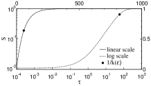
Figure 1: Source function $S(\epsilon,\tau^{*},\tau)$ in a slab with $\epsilon=10^{-4}$, $\tau^{*}=2000$. Right and top axes display the linear plot with infinite first derivative at $\tau=0$. Black dots show the thermalization depth $1/k(\epsilon)$ on both scales, the definition of $k(\epsilon)$ being given in Paper I.

The general behavior of the $S$-function is shown in Fig. 1, which illustrates the Table 3 of Paper I ($\epsilon=10^{-4}$ and $\tau^{*}=2000$). It can be seen that the solution $S$ tends to 1 for large values of $\tau$ and that it drops when $\tau$ is close to the thermalization depth $1/k(\epsilon)\approx 58$ for $\epsilon=10^{-4}$, where $k(\epsilon)$ is defined in Paper I. It tends steeply to the surface value $S(0)$ as $\tau$ tends to 0, with an infinite derivative at 0. It is regrettable that the generally adopted logarithmic scale in $\tau$ obscures this essential last point, as seen when comparing the solid and dashed curves of Fig. 1. The explanation lies in the fact that $\partial S/\partial(\log\tau)=\tau\,\partial S/\partial\tau\to 0$ even if $\partial S/\partial\tau\sim E_{1}(\tau)\to+\infty$.

4 Comparison with ALI numerical solutions

In this section we compare in detail the analytical solution described in the previous section to the one given by our ALI code. This code uses a diagonal approximate $\Lambda$-operator (Olson et al. 1986). At each iteration, a formal solver has to be used in order to calculate the transform of the source function by the $\Lambda$-operator. Inserting the definition (3) of the $E_{1}$-function into Eq. (2) and inverting the order of integrations, the so-called formal solution to the RTE is first calculated

$$I(\tau,\mu)=\left\{\!\begin{array}[]{ll}\displaystyle-\frac{1}{\mu}\!\int_{0}^{\tau}S(\tau^{\prime})\exp\left[(\tau-\tau^{\prime})/\mu\right]\,\mathrm{d}\tau^{\prime}&\rm if\;-1\leq\mu<0,\\ \displaystyle S(\tau)&\rm if\;\mu=0,\\ \displaystyle+\frac{1}{\mu}\!\int_{\tau}^{\tau^{*}}S(\tau^{\prime})\exp\left[-(\tau^{\prime}-\tau)/\mu\right]\,\mathrm{d}\tau^{\prime}&\rm if\;0<\mu\leq+1.\end{array}\right.$$ (13)

Then the $\Lambda$-transform of the source function is derived, since it is here the associated mean intensity

$$(\Lambda S)(\tau)=\frac{1}{2}\int_{-1}^{+1}I(\tau,\mu)\,\mathrm{d}\mu\,.$$ (15)

The formal solution (13) is calculated following the method of short characteristics whose basic elements can be found in Olson & Kunasz (1987) and Kunasz & Auer (1988). It was further improved by the implementation of monotonic interpolation for multi-dimensional applications (Auer & Paletou 1994) and by Fabiani Bendicho & Trujillo Bueno (1999) for three-dimensional applications with horizontal periodic boundary conditions. In the present paper, we used parabolic short characteristics. The $\mu$-integration in (15) is performed with the help of a Gaussian quadrature.

A numerical acceleration scheme is used so as to improve the rate of convergence of ALI: this is the so-called Ng-acceleration introduced in the field of radiative transfer by Auer (1987, 1991; see also Rybicki & Hummer 1991).

We have calculated the relative error

$$d(\epsilon,\tau^{*},\tau)=\left|\frac{S_{\mathrm{ALI}}(\epsilon,\tau^{*},\tau)-S(\epsilon,\tau^{*},\tau)}{S(\epsilon,\tau^{*},\tau)}\right|$$ (16)

at various optical depths, where $S(\epsilon,\tau^{*},\tau)$ is the analytical solution of Sec. 3 and $S_{\mathrm{ALI}}(\epsilon,\tau^{*},\tau)$ is the solution given by the ALI code. This error corresponds to the “true error” defined by Auer, Fabiani Bendicho & Trujillo Bueno (1994), who used a finer grid to calculate $S(\epsilon,\tau^{*},\tau)$.

We introduce also the maximum value of $d(\epsilon,\tau^{*},\tau)$ when the $\tau$-variable covers the domain $[0,\tau^{*}]$, viz.

$$d_{\mathrm{M}}(\epsilon,\tau^{*})=\max_{0\leq\tau\leq\tau^{*}}d(\epsilon,\tau^{*},\tau)\,.$$ (17)

Of course $d$ and $d_{\mathrm{M}}$ depend on the number of iterations $N$ performed by the ALI code during each run. Finally we define $N_{\mathrm{c}}$ as the number of iterations used to reach convergence, which is the smallest value of $N$ satisfying the condition $|1-d_{\mathrm{M}}(N)/d_{\mathrm{M}}(+\infty)|<\varepsilon_{\mathrm{c}}$, where $d_{\mathrm{M}}(+\infty)=d_{\mathrm{M}}(N=10\,000)$ and $\varepsilon_{\mathrm{c}}$ is arbitrarily set to $0.01$ in the present paper.

The slab optical depth is discretized using a logarithmic grid, symmetric with respect to the mid-plane, with $n_{\tau}$ points per decade, including the $\tau=0$ point, the next point denoted by $\tau_{\mathrm{m}}$, and the last point $\tau=\tau^{*}/2$. The angular integration in Eq. (15) is performed with a symmetric grid containing $n_{\mu}$ Gauss-Legendre points in $[0,1]$. There is no frequency integration since light scattering has been supposed monochromatic. In most of our calculations, we chose the values $\tau_{\mathrm{m}}=10^{-4}$, $n_{\tau}=9$, and $n_{\mu}=5$ (i.e., values quite often adopted for stellar atmospheres modelling). Some values of $(\epsilon,\tau^{*})$ may be (0.01, 20) for a continuum, ($10^{-4},2000$) for an “average” spectral line and ($10^{-8},2\times 10^{8}$) for a strong spectral line.

The quantities of interest are the maximum relative error $d_{\mathrm{M}}$ and the number of iterations to reach convergence $N_{\mathrm{c}}$, which depend on $\epsilon$, $\tau^{*}$ and numerical parameters $\tau_{\mathrm{m}}$, $n_{\tau}$, $n_{\mu}$ and $N$. We first study the variation of $d(\epsilon,\tau^{*},\tau)$ with $\tau$. Then, we study the influence of $\epsilon$, $\tau^{*}$, $n_{\tau}$ on $d_{\mathrm{M}}$ and $N_{\mathrm{c}}$, for given $\tau_{\mathrm{m}}$, $n_{\mu}$ and for $N=N_{\mathrm{c}}$.

4.1 The influence of $\tau$ and $N$

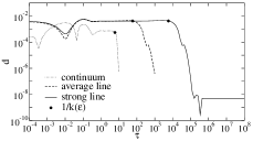
Figure 2: Relative error $d(\epsilon,\tau^{*},\tau)$ of the ALI code for $n_{\tau}=9$, $n_{\mu}=5$, $\tau_{\mathrm{m}}=10^{-4}$ and $N=1000$. Black dots show the thermalization depth $1/k(\epsilon)$ for each case.

Figure 2 shows the variation of the relative error $\tau\to d(\epsilon,\tau^{*},\tau)$ for the three selected values of $\epsilon$ and $\tau^{*}$. It can be seen that the accuracy (i.e. maximum relative error) of our ALI code is about $5\times 10^{-3}$ for the three cases studied here. Relative error is close to this accuracy when $\tau$ is smaller than the thermalization depth $1/k(\epsilon)$ of the atmosphere (black dots on the curves), and significantly improves beyond (up to $10^{-8}$). In photon mean free path units, the thermalization depth is 6, 58 and 5774 for $\epsilon=10^{-2},10^{-4}$ and $10^{-8}$ respectively. Note that the surface relative error is a good estimator of the accuracy in spectral lines, but not in the continuum.

Figure 3: Evolution of the maximum relative error $d_{\mathrm{M}}$ with iteration number $N$ for $n_{\tau}=9$, $n_{\mu}=5$ and $\tau_{\mathrm{m}}=10^{-4}$.

The iterative algorithm was stopped after $N=1000$ iterations. Figure 3 shows that this number ensures convergence of the ALI code, the convergence being slower when $\epsilon\to 0$ and $\tau^{*}\to+\infty$. Irregular steps in these curves are due to the Ng acceleration process, here operated every four iterations.

4.2 The influence of $\tau_{\mathrm{m}}$

We point out that $d_{\mathrm{M}}$ is improved when $\tau_{\mathrm{m}}$ goes to 0, up to a given value where the accuracy is constant. Including the $\tau=0$ point in the grid and choosing $\tau_{\mathrm{m}}<10^{-2}$, the best accuracy is warranted. Excluding the $\tau=0$ point from the grid has no influence on accuracy if we choose $\tau_{\mathrm{m}}<10^{-4}$. The standard choice $\tau_{\mathrm{m}}=10^{-4}$ is thus correct, and this value will be adopted hereafter.

4.3 The influence of $n_{\tau}$ and $n_{\mu}$

In Fig. 4 are shown the variations of $d_{\mathrm{M}}$ in an average line as a function of $n_{\tau}$ and $n_{\mu}$. The maximum relative error $d_{\mathrm{M}}$ decreases with increasing number $n_{\tau}$ of $\tau$-grid points, and it is sensitive to the choice of the number $n_{\mu}$ of angular grid points up to an optimal value $n_{\mu}^{\mathrm{(opt)}}$; the latter is defined as the smallest value of $n_{\mu}$ for which the condition $|1-d_{\mathrm{M}}(n_{\mu})/d_{\mathrm{M}}(64)|<0.01$ holds. The accuracy does not increase with a finer $\mu$-grid. We note that $n_{\mu}^{\mathrm{(opt)}}<n_{\tau}$ and that we have a linear dependence of this optimal value on $n_{\tau}$: $n_{\mu}^{\mathrm{(opt)}}=0.8n_{\tau}+2.7$ (dashed curve). This fit is still valid for strong lines.

As seen in Fig. 5 (same as Fig. 4 for the continuum), the fit for lines cannot be applied to the continuum, for which $n_{\mu}^{\mathrm{(opt)}}>n_{\tau}$. It is still possible to define and calculate an optimal value for $n_{\tau}<18$, using the relation $n_{\mu}^{\mathrm{(opt)}}=1.7n_{\tau}+1.3$ (dashed curve). It appears that our ALI code is more demanding in angular resolution when solving the problem (4) in a continuum than in a line.

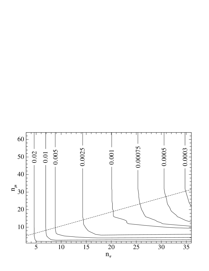
Figure 4: Maximum relative error $d_{\mathrm{M}}$ in an average line ($\tau^{*}=2000$, $\epsilon=10^{-4}$) as a function of $n_{\tau}$ and $n_{\mu}$. The dashed curve represents a linear fit $n_{\mu}^{\mathrm{(opt)}}=0.8n_{\tau}+2.7$.

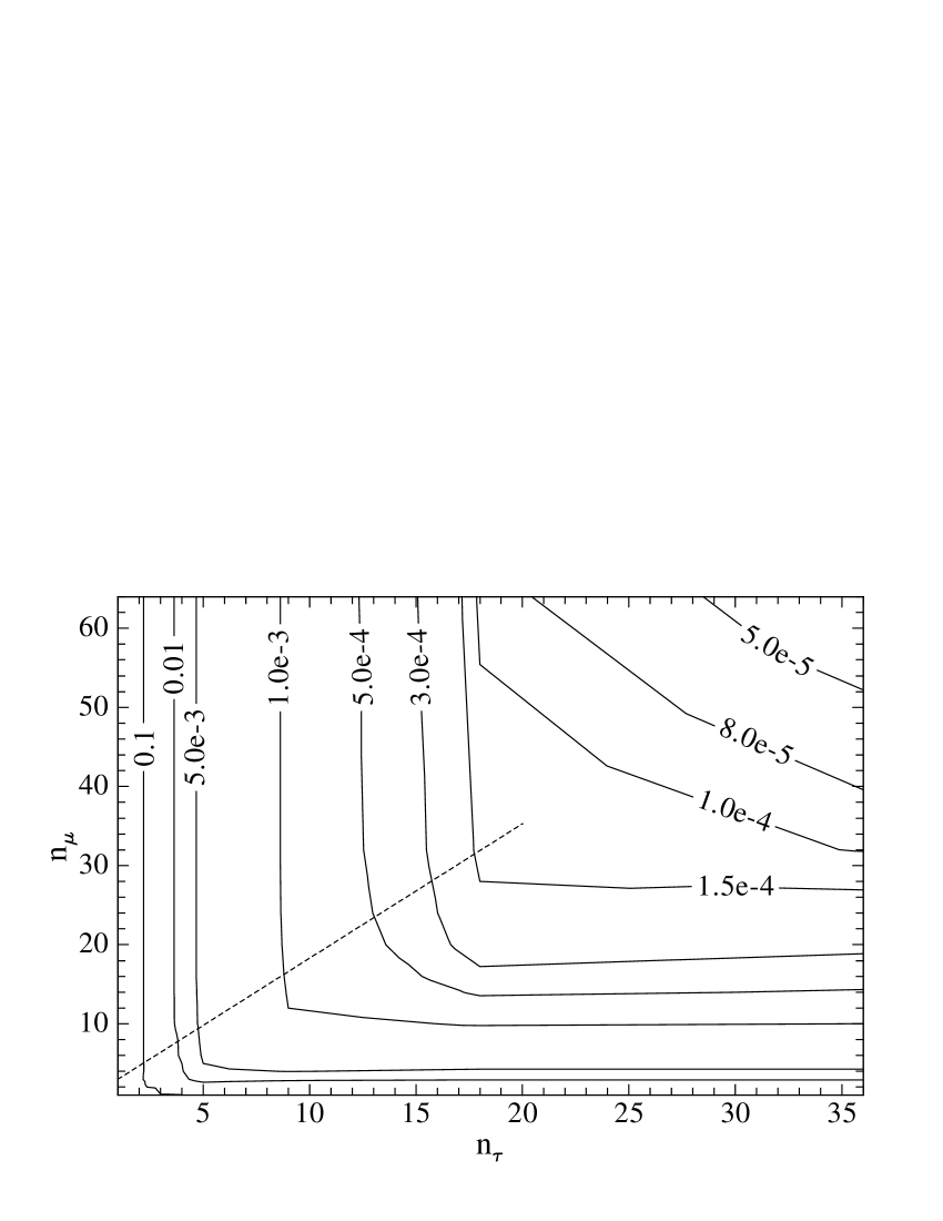
Figure 5: Maximum relative error $d_{\mathrm{M}}$ in the continuum ($\tau^{*}=20$, $\epsilon=0.01$) as a function of $n_{\tau}$ and $n_{\mu}$. Dashed curve represents a linear fit $n_{\mu}^{\mathrm{(opt)}}=1.7n_{\tau}+1.3$ for $n_{\tau}<18$.

The results of Figs. 4 and 5 are detailed in Fig. 6 for the three chosen values of $(\epsilon,\tau^{*})$ and $n_{\mu}=64$. We remark that the accuracy improves with $n_{\tau}$ for each couple $(\epsilon,\tau^{*})$, more significantly in the continuum than in lines.

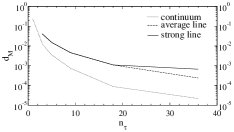
Figure 6: Maximum relative error $d_{\mathrm{M}}$ for different values of $n_{\tau}$ and $n_{\mu}=64$.

Figure 7: Number of iterations $N_{\mathrm{c}}$ used to reach convergence ($\varepsilon_{\mathrm{c}}=10^{-2}$) for different values of the parameter $n_{\tau}$ and $n_{\mu}=64$.

Figure 7 gives the number of iterations $N_{\mathrm{c}}$ used to reach convergence for $\varepsilon_{\mathrm{c}}=10^{-2}$ and $n_{\mu}=64$. The number $N_{\mathrm{c}}$ appreciably increases with $n_{\tau}$ in the lines: it is indeed well known that the rate of convergence of the one-point ALI iterative scheme drops for an increasing refinement of the spatial grid (Olson et al. 1986); however improvements were already proposed (e.g., Trujillo Bueno & Fabiani Bendicho 1995) in order to increase significantly the rate of convergence of ALI-based methods.

4.4 The influence of $\epsilon$ and $\tau^{*}$

The maximum relative error $d_{\mathrm{M}}$ and number of iterations $N_{\mathrm{c}}$ are shown in Figs. 8 and 9 for an extended range of $(\epsilon,\tau^{*})$ after the ALI code has converged ($N=10\,000$, $n_{\tau}=9$ and $n_{\mu}=5$ are fixed here).

As seen in Fig. 8, the accuracy hardly changes as $\epsilon\to 0$ and $\tau^{*}\to+\infty$, but the number of iterations needed to achieve convergence increases substantially (see Fig. 9). When $\epsilon>0.1$ the accuracy no longer depends on values of $\tau^{*}$. The comparison of Figs. 6 and 8 leads to a disagreement since the parameter $n_{\mu}$ is set to different values, 64 and 5 respectively.

In Fig. 9, we have plotted the parameter $N_{\mathrm{c}}$ as a function of $\epsilon$ and $\tau^{*}$. When $\epsilon\to 0$ and $\tau^{*}\to+\infty$, we note a slowing down of the convergence (already seen in Fig. 3).

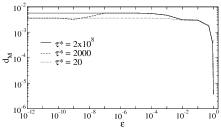
Figure 8: Maximum relative error $d_{\mathrm{M}}$ as a function of $\epsilon$ for parameters $n_{\tau}=9$ and $n_{\mu}=5$.

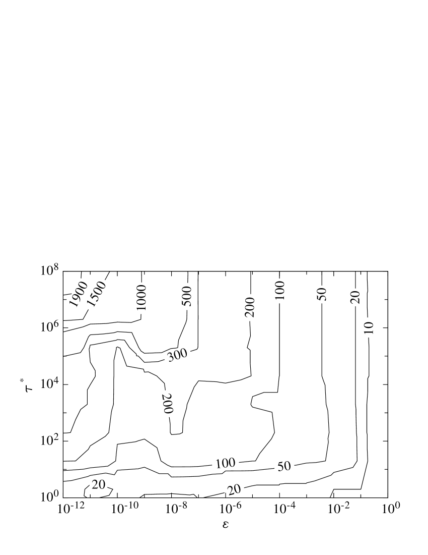
Figure 9: Number of iterations $N_{\mathrm{c}}$ ($\varepsilon_{\mathrm{c}}=10^{-2}$) as a function of $\epsilon$ and $\tau^{*}$ ($n_{\tau}=9$, $n_{\mu}=5$).

5 Comments on previous studies

Now we compare our results for the monochromatic scattering problem with those published by Trujillo Bueno & Fabiani Bendicho (1995) and Trujillo Bueno & Manso Sainz (1999). Although these two papers concern mainly the development of new iterative methods for radiative transfer applications (for the unpolarized and polarized cases respectively) they give some information on the accuracy of the numerical solutions obtained for spatial grids of increasing resolution.

In Table 1, good agreement is found between our values of $N_{\mathrm{c}}$, $d(\epsilon,\tau^{*},0)$ and those given by these authors; our surface relative error $d(\epsilon,\tau^{*},0)$ corresponds to their surface true error $T_{\mathrm{e}}$. The observed small discrepancies are possibly due to the different scattering laws adopted, leading to different $\Lambda$-operators.

Table 1: Comparison of results obtained with our (ALI+Ng) code and previous ones. Our $N_{\mathrm{c}}$ is defined by $\varepsilon_{\mathrm{c}}=0.01$, while values from other authors are based on a graphical guess $\varepsilon_{\mathrm{c}}\approx 0.05$. The optical thickness is $\tau^{*}=2\times 10^{8}$. Note that in Trujillo Bueno & Manso Sainz (1999), $N_{\mathrm{c}}$ values (in parenthesis) are given for a non-accelerated Jacobi scheme. These numbers have been divided by 2 in order to estimate the number of iterations when Ng acceleration is used.

$\epsilon,n_{\tau},n_{\mu}$	JTB & PFB (1995)		JTB & RMS (1999)		This article
	$N_{\mathrm{c}}$	$T_{\mathrm{e}}$	$N_{\mathrm{c}}$	surface $T_{\mathrm{e}}$	$N_{\mathrm{c}}$	$d_{\mathrm{M}}(\epsilon,\tau^{*})$	$d(\epsilon,\tau^{*},0)$
$10^{-6}$, 9, 1	180	$3.5\times 10^{-3}$			179	$8.6\times 10^{-2}$	$4.1\times 10^{-3}$
$10^{-12}$, 9, 1	1300	$3.5\times 10^{-3}$			985	$8.6\times 10^{-2}$	$4.1\times 10^{-3}$
$10^{-4}$, 5, 64			33 (65)	$2\times 10^{-2}$	42	$1.5\times 10^{-2}$	$1.3\times 10^{-2}$
$10^{-4}$, 9, 64			75 (150)	$3\times 10^{-3}$	88	$4.5\times 10^{-3}$	$3.9\times 10^{-3}$
$10^{-4}$, 18, 64			175 (350)	$4\times 10^{-4}$	184	$1.1\times 10^{-3}$	$9.0\times 10^{-4}$
$10^{-4}$, 36, 64			400 (800)	$5\times 10^{-5}$	356	$2.4\times 10^{-4}$	$1.9\times 10^{-4}$

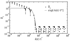
Figure 10: Relative difference $\delta_{1}=|1-S(\epsilon,\tau^{*},0)/\sqrt{\epsilon}|$ as a function of $k(\epsilon)\tau^{*}$. Dots represent values of $\epsilon\in[10^{-12},1]$ and $\tau^{*}\in[0.2,2\times 10^{8}]$, and the solid curve is $\exp\left(-k(\epsilon)\tau^{*}\right)$.

In Fig. 10 it is shown how far the semi-infinite exact result $S(\epsilon,0)=\sqrt{\epsilon}$ agrees with the finite one. This comparison is useful since many authors use the $\sqrt{\epsilon}$-law as a check for their calculations in thick slabs. We plot the relative difference $\delta_{1}=|\,1-S(\epsilon,\tau^{*},0)/\sqrt{\epsilon}\,|$ as a function of $k(\epsilon)\tau^{*}$, and the quantity $\exp\left(-k(\epsilon)\tau^{*}\right)$ which characterizes the validity of the $\sqrt{\epsilon}$-law (solid curve). For $k(\epsilon)\tau^{*}>100$, the accuracy limit of our code is reached, which explains that the solid curve no longer fits the dots. This law is very well satisfied in lines ($k(\epsilon)\tau^{*}\approx 34$ in an average line) but not enough in the continuum ($k(\epsilon)\tau^{*}\approx 3.3$). We conclude that the $\sqrt{\epsilon}$-law can be used as a test for the ALI code when $k(\epsilon)\tau^{*}>10$, since then $\sqrt{\epsilon}$ is an approximation to the surface value with an accuracy better than $10^{-4}$, as seen in Fig. 10.

In Trujillo Bueno & Fabiani Bendicho (1995), the Eddington approximation is used as the reference solution for a one-point angular quadrature $n_{\mu}=1$ with $\mu=\pm 1/\sqrt{3}$. The analytical expression of the Eddington approximation in a finite slab is:

$$S_{\mathrm{E}}(\epsilon,\tau^{*},\tau)=1-(1-\epsilon)\frac{\exp\left(-\sqrt{3\epsilon}\,\tau\right)+\exp\left(-\sqrt{3\epsilon}\,(\tau^{*}-\tau)\right)}{1+\sqrt{\epsilon}+(1-\sqrt{\epsilon})\exp\left(-\sqrt{3\epsilon}\,\tau^{*}\right)}.$$

This is the exact solution of the monochromatic scattering problem when the mean intensity is calculated with the above-mentioned one-point angular quadrature. However, as is well-known, it gives only an approximation to the exact (i.e., multi-angle) solution of the full problem (1)-(3). In other words, the true error given by Trujillo Bueno & Fabiani Bendicho (1995) is relative to the $n_{\mu}=1$ monochromatic scattering problem only, it does not give information on the error that would have been got by comparing the numerical solution to the $n_{\mu}=1,3,5,\ldots$ problem to the exact multi-angle solution ($n_{\mu}=\infty$). In fact, as given in Table 1 for $n_{\mu}=1$, when the solution of the $n_{\mu}=1$ problem is compared to the exact multi-angle solution, we find that the maximum error for $n_{\tau}=9$ is $8.6\times 10^{-2}$. The latter represents the maximum relative difference between the Eddington approximation and the exact solution (Fig. 11). A similar investigation, but for the two-level atom resonance-line scattering polarization problem, was carried out by Trujillo Bueno & Manso Sainz (1999), whose Table 3 gives the surface true-error values of the fractional atomic polarization for $n_{\mu}=3,5,7,11,\ldots,61$.

Figure 11: Variation with $\tau$ of the function $\delta_{2}(\epsilon,\tau^{*},\tau)=|1-S_{\mathrm{E}}(\epsilon,\tau^{*},\tau)/S(\epsilon,\tau^{*},\tau)|$ characterizing the accuracy of the Eddington approximation $S_{\mathrm{E}}$ as given by (5) for the usual three couples $(\epsilon,\tau^{*})$.

6 Conclusion

Our ALI code has been subjected to a wide range of tests, revealing at the same time its capabilities and its limits. Before developing these two points, we note that our conclusions are relative to the particular code we have used (based on Jacobi’s method), specifically solving the standard problem (1)-(3). The accuracy of the code is ultimately determined by the accuracy of the formal solver we have used (parabolic short characteristics).

We have checked the great robustness of our code, which is certainly its most remarkable feature. It is able to solve the standard problem (1)-(3) for a wide range of input parameters $\epsilon$ and $\tau^{*}$, with no important lack of performance when $\epsilon\to 0$ and/or $\tau^{*}\to+\infty$.

However, the lowest accuracy of the ALI numerical solutions happens in the outermost layers of a star, corresponding to $\tau$ lower than the thermalization depth $1/k(\epsilon)$, these layers forming, by definition, the atmosphere of the star. The accuracy of our code is not better than, say $10^{-2}$, when we choose $n_{\tau}=9$, $n_{\mu}=5$ and limit the number of iterations to $N<100$, as it is currently done in stellar atmospheres modelling. To improve the accuracy of the calculations up to $\sim 10^{-3}$, the parameters $n_{\tau}$, $n_{\mu}$ and $N$ should be set to larger (but today impractical) values when solving the radiative transfer equation on a large frequency spectrum, i.e. at thousands of frequencies. Indeed we pointed out a truly noticeable improvement of the accuracy when using finer grids in $\tau$ or $\mu$. Such an observation was made easier by the use of a very accurate reference solution. Of course, increasing the level of refinement of both spatial and angular quadratures has a strong impact upon the number of iterations needed for convergence. However, to overcome this difficulty while keeping the same accuracy on the numerical solutions, methods based on Gauss-Seidel and successive over-relaxation iterations were already proposed by Trujillo Bueno & Fabiani Bendicho (1995).

Another important question is relative to the propagation of errors in a stellar atmosphere model: to what extent are the main quantities provided by the model (populations of heavy particles, electron density, pressure, etc.) sensitive to the accuracy on the RTE solution? We intend to tackle this subject in a future work by constructing an accurate – but still very idealized – stellar atmosphere model, in which the main quantities are first derived from an exact solution to the RTE, and then from the solution given by a ALI-based numerical method.

- (1) Auer, L. H. 1987, in Numerical Radiative Transfer, ed. W. Kalkofen (Cambridge: Cambridge Univ. Press), 101
- (2) Auer, L. H. 1991, in NATO ASI Ser. C, Stellar Atmospheres: Beyond Classical Models, ed. L. Crivellari, I. Hubeny, & D. G. Hummer (Dordrecht: Kluwer), 9
- (3) Auer, L. H., & Paletou, F. 1994, A&A, 285, 675
- (4) Auer, L. H., Fabiani Bendicho, P., & Trujillo Bueno J. 1994, A&A, 292, 599
- (5) Chandrasekhar, S. 1960, Radiative Transfer, 2nd edn. (New York: Dover)
- (6) Chevallier, L., & Rutily, B. 2003, Exact solution of the standard transfer problem in a stellar atmosphere, A&A, submitted (Paper I)
- (7) Fabiani Bendicho, P., & Trujillo Bueno, J. 1999, Solar Polarization, ed. K.N. Nagendra & J.O. Stenflo, ASSL 243, 219
- (8) Hubeny, I. 2003, in ASP Conf. Ser. 288, Stellar Atmosphere Modeling, ed. I. Hubeny, D. Mihalas & K. Werner, 17
- (9) Ivanov, V.V. 1973, Transfer of radiation in spectral lines, National Bureau of Standards Special Publication 385, U. S. Government Printing Office
- (10) Kunasz, P. B., & Auer, L. H. 1988, J. Quant. Spectros. Radiat. Transfer, 39, 67
- (11) Mihalas, D. 1978, Stellar Atmospheres, 2nd edn. (San Francisco: Freeman and Co)
- (12) Olson, G. L., Auer, L. H., & Buchler, J. R. 1986, J. Quant. Spectros. Radiat. Transfer, 35, 431
- (13) Olson, G.L., & Kunasz, P.B. 1987, J. Quant. Spectros. Radiat. Transfer, 38, 325
- (14) Paletou, F. 2001, C. R. Acad. Sci. Paris, Serie IV, t. 2, 6, 885
- (15) Rybicki, G. B., & Hummer, D. G. 1991, A&A, 245, 171
- (16) Sobolev, V. V. 1957, Dokl. Akad. Nauk SSSR, 116, 45 [Sov. Phys. Dokl., 2, 426]
- (17) Sobolev, V. V. 1958, Dokl. Akad. Nauk SSSR, 120, 69 [Sov. Phys. Dokl., 3, 541]
- (18) Trujillo Bueno, J., & Fabiani Bendicho, P. 1995, ApJ, 455, 646
- (19) Trujillo Bueno, J., & Manso Sainz, R. 1999, ApJ, 516, 436
- (20) Trujillo Bueno, J. 2003, in ASP Conf. Ser. 288, Stellar Atmosphere Modeling, ed. I. Hubeny, D. Mihalas & K. Werner, 551
- (21) Van de Hulst, H. C. 1980, Multiple Light Scattering, vol. 1 (New York: Academic Press)