BARRED GALAXIES: STUDYING THE CHAOTIC AND ORDERED NATURE OF ORBITS

Abstract

The chaotic or ordered character of orbits in galactic models is an important issue, since it can influence dynamical evolution. This distinction can be achieved with the help of the Smaller ALingment Index - (SALI). We describe here briefly this method and its advantages. Then we apply it to that case of 2D and 3D barred galaxy potentials. In particular, we find the fraction of chaotic and ordered orbits in such potentials and present how this fraction changes when the main parameters of the model are varied. For this, we consider models with different bar mass, bar thickness or pattern speed. Varying only one parameter at a time, we find that bars that are more massive, or thinner, or faster, have a larger fraction of chaotic orbits.

1 INTRODUCTION

The chaotic and ordered motion in dynamical systems is a very important issue in non - linear sciences in general and in dynamical astronomy in particular. The qualitative distinction of the motion is, generally, not that trivial and it becomes harder in systems of many degrees of freedom. Thus, it is necessary to use fast and precise methods to indicate the nature of the orbits.

Many methods have been developed over the years trying to give an answer to this problem. The inspection of the successive intersections of an orbit with a Poincaré surface of section (PSS) LL has been used mainly for 2 dimensional (2D) maps and 2 degrees of freedom Hamiltonian systems. One of the most common methods of chaos detection is the computation of the ”Maximal Lyapunov Characteristic Number” (LCN) Fro:1 ,Ben:1 , which can be applied for systems with many degrees of freedom. Another very efficient method is the ”Frequency Map Analysis” Las:1 ,Las:2 . In recent years new methods have been introduced such as the study of spectra of ”Short Time Lyapunov Characteristic Numbers” Fro:2 ,Loh:1 or ”Stretching Numbers” Vog:1 ,Con:1 and the ”Spectral Distance” of such spectra Vog:2 , as well as the study of spectra of helicity and twist angles Con:2 ,Con:3 ,Fro:3 . In addition, Froeschlé, Lega & Gonzi Fro:4 introduced the ”Fast Lyapunov Indicator” (FLI), while Vozikis, Varvoglis & Tsiganis Voz:1 proposed a method based on the frequency analysis of ”Stretching Numbers”.

Recently, a new, fast and easy to compute indicator of the chaotic or ordered nature of orbits, has been introduced sk:1 and was applied successfully in different dynamical systems sk:1 ,sk:2 ,sk:3 ,sk:4 ,sk:5 ,Pan:1 ,Ant:1 ,SESS , the so-called ”Smaller Alignment Index (SALI)”, or, as elsewhere called Alignment Index (AI) VKS ,KVC . In the present paper, we first recall its definition and then we show its effectiveness in distinguishing between ordered and chaotic motion, by applying it to a barred potential of 2 and 3 degrees of freedom.

2 DEFINITION OF THE SMALLER ALIGNMENT INDEX

Let us consider the $n$ - dimensional phase space of a conservative dynamical system, which could be a symplectic map or a Hamiltonian flow. We consider also an orbit in that space with initial condition $P(0)=(x_{1}(0),x_{2}(0),...,x_{n}(0))$ and a deviation vector $v(0)=(dx_{1}(0),dx_{2}(0),...,dx_{n}(0))$ from the initial point $P(0)$. In order to compute the SALI for a given orbit one has to follow the time evolution of the orbit with initial condition itself and also of two deviation vectors $v_{1}(t),v_{2}(t)$ which initially point in two different directions. The evolution of these deviation vectors is given by the variational equations for a flow and by the tangent map for a discrete-time system. At every time step the two deviation vectors $v_{1}(t)$ and $v_{2}(t)$ are normalized and the SALI is then computed as:

$$SALI(t)=min\left\{\left\|\frac{v_{1}(t)}{\|v_{1}(t)\|}+\frac{v_{2}(t)}{\|v_{2}(t)\|}\right\|,\left\|\frac{v_{1}(t)}{\|v_{1}(t)\|}-\frac{v_{2}(t)}{\|v_{2}(t)\|}\right\|\right\}.$$ (1)

The properties of the time evolution of the SALI clearly distinguish between ordered and chaotic motion as follows: In the case of Hamiltonian flows or dimensional symplectic maps with $n\geq 2$, the SALI fluctuates around a non-zero value for ordered orbits, while it tends to zero for chaotic orbits sk:1 ,sk:3 ,sk:4 . In the case of 2D maps the SALI tends to zero both for ordered and chaotic orbits, following however completely different time rates, which again allows us to distinguish between the two cases. In 2 and 3 degrees of freedom Hamiltonian systems the distinction between ordered and chaotic motion is easy because the ordered motion occurs on a 2D or 4D torus respectively on which any initial deviation vector becomes almost tangent after a short transient period. In general, two different initial deviation vectors become tangent to different directions on the torus, producing different sequences of vectors, so that SALI does not tend to zero but fluctuates around positive values. On the other hand, for chaotic orbits, any two initially different deviation vectors tend to coincide in the direction defined by the nearby unstable manifold and hence either coincides with each other, or become opposite. This means that the SALI tends to zero when the orbit is chaotic and to a non-zero value when the orbit is ordered. Thus, the completely different behavior of the SALI helps us to distinguish between ordered and chaotic motion in Hamiltonian systems with 2 and 3 degrees of freedom and in general in dynamical systems of higher dimensionality.

3 THE MODEL

A 3D rotating bar model can be described by the Hamiltonian function:

$$H=\frac{1}{2}(p_{x}^{2}+p_{y}^{2}+p_{z}^{2})+V(x,y,z)-\Omega_{b}(xp_{y}-ypx_{x}),$$ (2)

where $x$ is the long axis, $y$ the intermediate and $z$ the short axis around which the bar rotates. The $p_{x},p_{y}$ and $p_{z}$ are the canonically conjugate momenta. Finally, $V$ is the potential, $\Omega_{b}$ represents the pattern speed of the bar and $H$ is the total energy of the system.

The potential of the model $V$ consists of three components:

a) A disc, represented by a Miyamoto disc Miy.1975 :

$$V_{D}=-\frac{GM_{D}}{\sqrt{x^{2}+y^{2}+(A+\sqrt{z^{2}+B^{2}})^{2}}}.$$ (3)

where $M_{D}$ is the total mass of the disc, $A$ and $B$ are the horizontal and vertical scalelengths, and $G$ is the gravitational constant.

b) The bulge is modeled by a Plummer sphere with the potential:

$$V_{S}=-\frac{GM_{S}}{\sqrt{x^{2}+y^{2}+z^{2}+\epsilon_{s}^{2}}}$$ (4)

where $\epsilon_{s}$ is the scalelength of the bulge and $M_{S}$ is its total mass.

c) The triaxial Ferrers bar, the density $\rho(x)$ of which is:

$$\rho(x)=\begin{cases}\rho_{c}(1-m^{2})^{2}&,m<1\\ \qquad 0&,m\geq 1\end{cases},$$ (5)

where $\rho_{c}=\frac{105}{32\pi}\frac{GM_{B}}{abc}$ the central density, $M_{B}$ is the total mass of the bar and

$$m^{2}=\frac{x^{2}}{a^{2}}+\frac{y^{2}}{b^{2}}+\frac{z^{2}}{c^{2}},\qquad a>b>c\geq 0,$$ (6)

with $a,b$ and $c$ are the semi-axes and $M_{B}$ the mass of the bar component. The corresponding potential $V_{B}$ and the forces are given in D. Pfenniger (1984) Pfe .

3.1 Applications in the 2D case

We first apply the SALI index to the 2 degrees of freedom barred potential. In this case, we can have a Poincaré Surface of Section (PSS) and can check the effectiveness of the SALI, by comparing the results.

In figure 1, we present two orbits of different kind: (i) $(x,y,p_{x},p_{y})=(1.5,0,p_{x}(H),0)$ and (ii) $(x,y,p_{x},p_{y})=(-0.9,0,p_{x}(H),0)$. For this application $H=-0.3$. In panels a) and b) of figure 1, we show the orbit projections in the $(x,y)$-plane and in panel c) we draw their corresponding PSS, where we can see that the chaotic orbit (i) tends to fill with scattered points the available part of the $(x,\dot{x})$ plane and that the ordered orbit (ii) creates a closed invariant curve. Finally, in panel d) we apply the SALI method for these two orbits. For the chaotic one, the SALI tends to zero $(10^{-16})$ exponentially after some time steps while for the regular orbit, it fluctuates around a positive number. By choosing initial conditions on the line $\dot{x}=0$ of the PSS and calculating the values of the SALI, we can detect very small regions of stability that can not be visualized easily by the PSS method. Repeating this for many values of the energy, we are able to follow the change of the fraction of chaotic and ordered orbits in the phase space as the energy of the orbit varies.

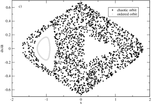
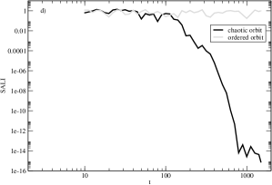
Figure 1: Projections of the orbits (i) and (ii) in the $(x,y)$-plane (panels a), b)). PSS of these two orbits in panel c). Behaviour of the SALI of the same orbits (panel d)).

3.2 Applications in the 3D case

In figure 2 we present percentages of chaotic, intermediate and regular trajectories, where we vary the mass of the bar component (panels A3-B3) and the length of the short $z$-axis (panels A2-B2) of the initial models A1 and B1. The two rows differ in the way we give the 27000 initial conditions. For the A1, we give initial conditions in the plane $(x,p_{y},z)$ with $(y,p_{x},p_{z})=(0,0,0)$ and for the B1, in the plane $(x,p_{y},p_{z})$ with $(y,z,p_{x})=(0,0,0)$. By comparing the results, we see that the increase of the bar mass causes more chaotic behavior in both cases (panels A3, B3). This confirms the results by Athanassoula et al. (1983) ABMP in 2 degrees of freedom. On the other hand, it is obvious

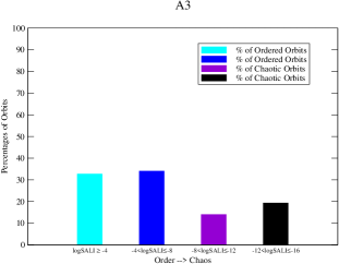
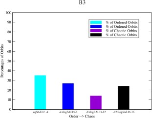
Figure 2: Percentages of regular (first and second bar) and chaotic (third and forth bar) orbits, for our standard model (first row of panels), a model with a thick bar (second row) and a model with a massive bar (third row). The two columns show two different ways of choosing the orbital population.

that when the bar is thicker, i.e. the length of the $z$-axis larger, the system gets more regular.

Finally, we calculated the same percentages for different pattern speeds $\Omega_{b}$. From the orientation of periodic orbits, Contopoulos (1980) Con:4 showed that bars have to end before corotation, i.e. that $r_{L}>a$, where $r_{L}$ the Lagrangian, or corotation, radius. Comparing the shape of the observed dust lanes along the leading edges of bars to that of the shock loci in hydrodynamic simulations of gas flow in barred galaxy potentials, Athanassoula (1992a,b) Athan:2 ,Athan:3 was able to set both a lower and an upper limit to corotation radius, namely $r_{L}=(1.2\pm 0.2)a$. This restricts the range of possible values of the pattern speed, i.e. $\Omega_{b}=0.0367032$, that corresponds to the Lagrangian radius $r_{L}=1.4a$ and $\Omega_{b}=0.0554349$, that corresponds to $r_{L}=1.0a$. Using the extremes of this range, we investigated how the pattern speed of the bar affects the system and found that the percentage of the regular orbits is greater in slow bars.

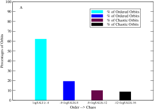
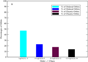
Figure 3: The percentages of the chaotic and ordered orbits for the two different values of the pattern speeds. Panel A corresponds to $\Omega_{b}=0.0367032$ and panel B to $\Omega_{b}=0.0554349$. The latter presents more chaotic behavior.

4 CONCLUSIONS

In this paper, we applied the SALI method in the Ferrers barred galaxy models of 2 and 3 degrees of freedom. We presented and discussed our results comparing the SALI index with traditional methods, such as the PSS method for the 2 degrees of freedom and showed its effectiveness. We also, calculated percentages of chaotic and regular orbits and how they change with the main model parameters, for the 3 degrees of freedom case. In more detail, we calculated percentages of chaotic and ordered trajectories, as some important parameters, as the mass, the length of the short $z$-axis and the pattern speed of the bar vary in the initial basic model.

References

- (1) M. Lieberman and A. Lichtenberg, Springer Verlag, (1992).
- (2) C. Froeschlé, Cel. Mech., 34, 95, (1984).
- (3) G. Benettin, L. Galgani and J.M. Strelcyn, Phys. Rev. A, 14, 2338, (1976).
- (4) J. Laskar, Icarus, 88, 266, (1990).
- (5) J. Laskar, C. Froeschlé and A. Celletti, Physica D, 56, 253, (1992).
- (6) C. Froeschlé, Ch. Froeschlé and E. Lohinger, Celest. Mech. Dyn. Astron., 56, 307, (1993).
- (7) E. Lohinger, C. Froeschlé and R. Dvorak, Celest. Mech. Dyn. Astron., 56, 315, (1993).
- (8) N. Voglis and G. Contopoulos J. Phys. A, 27, 4899, (1994).
- (9) G. Contopoulos, E. Grousousakou and N. Voglis, Astr. Astroph., 304, 374, (1995).
- (10) N. Voglis, G. Contopoulos and C. Efthymiopoylos, Celest. Mech. Dyn. Astron., 73, 211, (1999).
- (11) G. Contopoulos and N. Voglis, Celest. Mech. Dyn. Astron., 64, 1, (1996).
- (12) G. Contopoulos and N. Voglis, Astr. Astroph., 317, 73, (1997).
- (13) C. Froeschlé and E. Lega, Astr. Astroph., 334, 355, (1998).
- (14) C. Froeschlé, E. Lega and R. Gonzi, Celest. Mech. Dyn. Astron., 67, 41, (1997).
- (15) Ch. L. Vozikis, H. Varvoglis and K. Tsiganis, Astr. Astroph., 359, 386, (2000).
- (16) Ch. Skokos, J. Phys. A: Math. Gen., 34, 10029, (2001).
- (17) Ch. Skokos, C. Antonopoulos, T. Bountis and M. Vrahatis, in Proceedings of the 4th GRACM, edited by D. T. Tsahalis, IV, 1496. (2002).
- (18) Ch. Skokos, C. Antonopoulos, T. Bountis and M. Vrahatis, Prog. Theor. Phys. Suppl., 150, 439, (2003).
- (19) Ch. Skokos, C. Antonopoulos, T. Bountis and M. Vrahatis, in Proceedings of the Conference Libration Point Orbits and Applications, edited by G. Gomez, M. W. Lo and J. J. Masdemont , World Scientific, 653, (2003).
- (20) Ch. Skokos, C. Antonopoulos, T. Bountis and M. Vrahatis, J. Phys. A, 37, 6269, (2004).
- (21) P. Panagopoulos, T. Bountis and Ch. Skokos, J. Vib. & Acoust., 126, 520, (2004).
- (22) C. Antonopoulos, T. Manos and Ch. Skokos, in Proceedings of the 1st IC-SCCE, edited by D. T. Tsahalis, Patras Univ. Press, III, 1082, (2005).
- (23) A. Széll, B. Érdi, Zs. Sándor and B. Steves, Mon. Not. R. Astron. Soc., 347, 380, (2004).
- (24) N. Voglis , C. Kalapotharakos and I. Stavropoulos, Mon. Not. R. Astron. Soc., 337, 619, (2002).
- (25) C. Kalapotharakos , N. Voglis and G. Contopoulos, Mon. Not. R. Astron. Soc., 428, 905, (2004).
- (26) M. Miyamoto and R. Nagai, PASJ, 27, 533, (1975).
- (27) D. Pfenniger, Astr. Astroph., 134, 373, (1984).
- (28) E. Athanassoula , O. Bienayme, L. Martinet and D. Pfenniger, Astr. Astroph, 127, 349, (1983).
- (29) G. Contopoulos, Astr. Astroph, 81, 198, (1980).
- (30) E. Athanassoula, Mon. Not. R. Astron. Soc., 259, 328, (1992a).
- (31) E. Athanassoula, Mon. Not. R. Astron. Soc., 259, 354, (1992b).