Stacking weak lensing signals of SZ clusters to constrain cluster physics

Abstract

We show how to place constraints on cluster physics by stacking the weak lensing signals from multiple clusters found through the Sunyaev-Zeldovich (SZ) effect. For a survey that covers about $200$ sq. deg. both in SZ and weak lensing observations, the slope and amplitude of the mass vs. SZ luminosity relation can be measured with few percent error for clusters at $z\sim 0.5$. This can be used to constrain cluster physics, such as the nature of feedback. For example, we can distinguish a pre-heated model from a model with a decreased accretion rate at more than 5$\sigma$. The power to discriminate among different non-gravitational processes in the ICM becomes even stronger if we use the central Compton parameter $y_{0}$, which could allow one to distinguish between models with pre-heating, SN feedback and AGN feedback, for example, at more than 5$\sigma$. Measurement of these scaling relations as a function of redshift makes it possible to directly observe e.g., the evolution of the hot gas in clusters. With this approach the mass-L_SZ relation can be calibrated and its uncertainties can be quantified, leading to a more robust determination of cosmological parameters from clusters surveys. The mass-L_SZ relation calibrated in this way from a small area of the sky can be used to determine masses of SZ clusters from very large SZ-only surveys and is nicely complementary to other techniques proposed in the literature.

1. Introduction

Clusters of galaxies are powerful probes of cosmology. In particular, the cluster number density as a function of mass and redshift can provide unique constraints on the growth of cosmological structure and e.g. on dark energy.

The next generation of Sunyaev-Zel’dovich (SZ) surveys, e.g., the Atacama Cosmology Telescope (ACT) and the South Pole Telescope (SPT), will provide a catalog of thousands of clusters. The flux of the SZ is proportional to the integral of the density times the temperature of the hot gas in the cluster (Sunyaev & Zeldovich, 1980) and the flux limit of the catalogs will approximately translate into a mass limit. However, the actual value of the cluster’s mass for a given SZ flux depends on the details of the SZ-mass relation, which in turn is governed by cluster physics.

Recent work has shown how this relation can be obtained by using numerical simulations (e.g. Oh & Benson (2003); da Silva et al. (2004); Motl et al. (2005); Nagai (2005)) or analytical approximations (e.g. Dos Santos & Dore (2001); Reid & Spergel (2005); Roychowdhury et al. (2005); Ostriker et al. (2005)). Numerical models find that the SZ-mass relation is expected to be very tight, implying that clusters masses can be directly read out from the SZ observations once the SZ-mass relation has been calibrated. In addition, both numerical work and analytical approximations have shown that the integrated SZ luminosity of a cluster is relatively insensitive to input physics used in the models, such as pre-heating and energy injection by supernovae or Active Galactic Nuclei (e.g. Motl et al. (2005); Nagai (2005); Lapi et al. (2005)). The same models, however, show a larger scatter with mass of the central SZ decrement parameter ($y_{0}$) and a much stronger dependence of $y_{0}$ on the cluster physics.

Ideally, we would like an independent and robust measurement of the cluster mass from observations. This would open the possibility to not just calibrate the SZ-mass relation directly from observations, but also to test intra-cluster medium (ICM) models, and therefore to directly probe cluster physics. Arguably, weak gravitational lensing provides a direct way to measure the mass of clusters. The distortions of the background galaxies due to the cluster’s gravitational field are sensitive to the mass along the line of sight, not just the intra-cluster gas. These distortions can be used to reconstruct the cluster’s projected mass density (e.g., Kaiser & Squires (1993)).

The weak lensing signal induced by galaxy clusters has been measured for a large number of systems (e.g., Clowe et al. (2005); Sheldon et al. (2001) and references therein). The amplitude of the lensing signal depends on the redshift distribution of the faint background galaxies, which can be obtained from photometric observations. Observations from the ground are limited by the atmosphere: both the maximum surface density of background galaxies and the minimum error on the shear are set by the seeing. While observations from space could circumvent this difficulty, there is no wide-field imager available in the near future to do this (ACT will cover a region of a few hundred sq. deg. and SPT 4000 sq. deg.). As both these factors set the minimum cluster mass that can be directly detected from weak lensing, a direct mass determination is possible only for fairly massive clusters, $\approx 10^{15}\rm M_{\odot}$ (e.g., Marian & Bernstein (2005)).

Here we circumvent this limitation by taking advantage of the wide multi-wavelength coverage provided by ACT and SPT with their planned extensive optical follow up (Southern Cosmology Survey and Dark Energy Survey). By combining (stacking) the weak lensing signals from multiple clusters with roughly the same SZ luminosity, otherwise undetectable shear signal can be amplified, and thus an average mass determination can be achieved.

The goal of this paper is to quantify the error in the calibration of the mass-SZ relation achievable by stacking weak lensing observations of SZ clusters. This also will allow one to investigate cluster physics since the scatter and amplitude in the SZ-mass relation can then be directly compared with predictions from numerical simulations. In addition, a well calibrated mass$-$SZ relation can lead to a more robust determination of cosmological parameters from cluster surveys.

Here, we will consider what can be learned by stacking clusters from a survey with the specifications of the two-year ACT SZ survey, assuming that the entire clean region (200 sq. deg.) is covered by optical weak lensing observations with a seeing of $\sim 0.6$ to $0.7$ arcsec and $20$ source galaxies per square arcminute. The outline of the paper is as follows: in section 2 we compute the expected error in the mass estimator for the stacked clusters. In section 3 we explore how cluster physics can be constrained with the mass-SZ relation calibrated from the finding of section 2. We conclude in section 4 where we also outline the possible consequences of this approach for constraining the evolution of the hot gas in clusters and for obtaining a more robust determination of cosmological parameters from clusters surveys.

2. Combining lensing signals from multiple clusters

In ground-based experiments, the cluster weak lensing signal is smaller than the noise for masses less than $10^{15}$ $\rm M_{\odot}$, due to the low number density of background galaxies and the error with which their sheer can be measured. Here we illustrate how the weak lensing signal from multiple lower–mass clusters can be combined to increase the signal-to-noise ($S/N$) ratio. In particular, we will consider measuring the average mass of several clusters in a given redshift bin and mass range. We follow closely Marian & Bernstein (2005) and define our average mass estimator as the weighted sum:

$$M=\sum_{d,k,s}w_{ks,d}\gamma_{T}(R_{k},z_{s},z_{d})$$ (1)

where $d$ is the index of the stacked clusters, and $\gamma_{T}$ denotes the average tangential shear of source galaxies in redshift bin $s$ in an annulus with physical radius $R_{k}$ in the plane of lens $d$, and $w_{ks,d}$ are the weights, which should be chosen e.g., to maximize $S/N$. This is the same as the mass estimator used by Marian & Bernstein (2005), but here it includes a weighted sum over different clusters, and the tangential shear is in physical rather than angular annuli.

The variance of this mass estimator is

$$\sigma_{M}^{2}=\sum_{d,k,s}w_{ks,d}^{2}\sigma^{2}_{\gamma_{T}}(R_{k},z_{s},z_{d}).$$ (2)

The weights $w_{ks,d}$ that maximize $S/N$ are,

$$w_{ks,d}=\left[\frac{\sum_{i,j,l}w_{ij,l}\gamma_{T}}{\sum_{ij,l}w_{ij,l}^{2}\sigma^{2}_{\gamma_{T}}}\right]\frac{\gamma_{T}(R_{k},z_{s},z_{d})}{\sigma^{2}_{\gamma_{T}}(R_{k},z_{s},z_{d})}$$ (3)

The term in square brackets is constant for all $k,s$ and $d$. Denoting this normalization constant by $\mathcal{A}$, clearly

$$\mathcal{A}=\frac{M}{\sum_{k,s,d}\frac{\gamma_{T}^{2}}{\sigma^{2}_{\gamma_{T}}}}$$ (4)

which yields

$$\sigma_{M}^{2}=M^{2}\left(\sum_{k,s,d}\frac{\gamma_{T}^{2}(R_{k},z_{s},z_{d})}{\sigma^{2}_{{\gamma_{T}}_{k,s,d}}}\right)^{-1}$$ (5)

Like Marian & Bernstein (2005); Bartelmann & Schneider (2001), we define $Z(z_{s},z_{d})\equiv\frac{D_{ds}}{D_{s}}\Theta(z_{s}-z_{d})$ where $\Theta$ is the unit step function. The shear per unit mass for a hypothetical source at infinity is,

$$\tilde{\gamma}_{\infty}(\theta_{k},z_{d})=\frac{\gamma_{T}(R_{k},z_{s},z_{d})}{MZ(z_{s},z_{d})}$$ (6)

The variance of $\gamma_{T}$ from $N$ galaxies in annulus $k$ and redshift bin $s$ is approximated by $\sigma_{\gamma}^{2}/N$ and $\sigma_{\gamma}$ is assumed constant. We also assume a constant number density $n_{g}$ of galaxies per unit solid angle on the sky, distributed in redshift according to a Poisson distribution,

$$\mathcal{P}(z_{s})=\frac{1}{2z_{0}^{3}}z_{s}^{2}e^{\frac{-z_{s}}{z_{0}}}.$$ (7)

The number of galaxies in an annulus of thickness $d\theta$ is $2\pi n_{g}\sin\theta\,d\theta$, where $\theta=R/D_{d}$, so the number of galaxies in a physical annulus per unit redshift of a cluster at redshift $z_{d}$ is $2\pi n_{g}\mathcal{P}(z_{s})\sin\left(\frac{R}{D_{d}}\right)/D_{d}\,dR\,dz_{s}$.

Taking the continuous limit of the summation over $k,s$ in Eq. 5, and $R\ll D_{d}$, we obtain

$$\sigma_{M}^{2} = \frac{\sigma_{\gamma}^{2}}{2\pi n_{g}}$$

$$\times \frac{1}{\sum_{d}\int_{0}^{\infty}dz_{s}\mathcal{P}(z_{s})Z^{2}(z_{s},z_{d})\int_{0}^{R_{\mathrm{lim}}}\frac{R}{D_{d}^{2}}dR\theta\,\tilde{\gamma}_{\infty}^{2}(R,z_{d})}$$

$$= \left(\sum_{d}\frac{1}{\sigma^{2}_{d}}\right)^{-1},$$ (9)

where $\sigma^{2}_{d}$ is the contribution to the variance from a single lens at redshift $z_{d}$, as derived by Marian & Bernstein (2005). Thus, as intuitively expected, if one were to stack $N$ identical clusters (clusters with the same mass at the same redshift) the density of background galaxies would increase by a factor $N$ and thus the error on the measured mass would decrease by a factor $\sqrt{N}$.

2.1. Cluster profiles

We assume a NFW radial cluster profile (Navarro et al., 1997),

$$\rho(r)=\frac{\rho_{s}}{(r/r_{s})(1+r/r_{s})^{2}}.$$ (10)

We set $\rho_{s}$ and $r_{s}$ according to the clusters mass and redshift, using the fitting formulae from Bullock et al. (2001); Bryan & Norman (1998).

$$\rho_{s}(z,\mathcal{C})=\frac{1}{3}\delta_{\mathcal{C}}(\mathcal{C})\Delta(z)\rho_{\mathrm{cr}}(z)$$ (11)

$$\Delta(z)=18\pi^{2}+82(\Omega(z)-1)-39(\Omega(z)-1)^{2}$$ (12)

$$\delta_{\mathcal{C}}=\frac{\mathcal{C}^{3}}{\ln(1+\mathcal{C})-\mathcal{C}/(1+\mathcal{C})}$$ (13)

$$r_{s}(M_{\mathrm{vir}},z)=\frac{r_{\mathrm{vir}}(M_{\mathrm{vir}})}{\mathcal{C}(M_{\mathrm{vir}},z)}$$ (14)

$$\mathcal{C}(M_{\mathrm{vir}},z)=\frac{9.6}{\left(\frac{M_{\mathrm{vir}}}{M_{*}(z)}\right)^{0.13}(1+z)}$$ (15)

$$\sigma(M_{*})=\frac{1.686}{G(z)}$$ (16)

where $G(z)$ is the linear growth rate and $\mathcal{C}$ is the concentration parameter, $\Omega(z)$ is the ratio of the mean matter density to $\rho_{\mathrm{cr}}(z)$, $\rho_{\mathrm{cr}}(z)$ is the critical density of the universe at redshift $z$, and $\sigma^{2}(M)$ is the linear density field variance smoothed with a top-hat filter. The mass is related to the virial radius by

$$M\equiv M_{\mathrm{vir}}=\frac{4\pi}{3}\Delta(z)\rho_{\mathrm{cr}}(z)r_{\mathrm{vir}}^{3}.$$ (17)

The tangential shear is given by Wright & Brainerd (2000):

$$\gamma_{NFW}=\frac{r_{s}\delta_{\mathcal{C}}\rho_{\mathrm{cr}}}{\Sigma_{\mathrm{cr}}}g(x)$$ (18)

$$\Sigma_{\mathrm{cr}}=\frac{c^{2}}{4\pi G}\frac{D_{s}}{D_{d}D_{ds}}$$ (19)

where $x=\frac{R}{r_{s}}$. Thus $\tilde{\gamma}_{\infty}$ becomes

$$\tilde{\gamma}_{\infty}=\frac{3G}{\Delta(D_{d})c^{2}}\frac{D_{d}\delta_{\mathcal{C}}}{r_{s}^{2}\mathcal{C}^{3}}g(x).$$ (20)

Following Marian & Bernstein (2005), we take the upper limit of the second integral in Eq.2 to be $R_{\mathrm{lim}}=2r_{\mathrm{vir}}$, obtaining

$$\int_{0}^{R_{\mathrm{lim}}}\frac{R}{D_{d}^{2}}dR\tilde{\gamma}_{\infty}^{2}(R)=\left(\frac{3G}{\Delta c^{2}}\right)^{2}\frac{\delta_{\mathcal{C}}^{2}}{r_{s}^{2}\mathcal{C}^{6}}\int_{0}^{2\mathcal{C}}xdxg^{2}(x)\,.$$ (21)

If we denote the numbers of clusters per unit redshift per unit mass per steradian as $n_{c}(M,z)$, and the fraction of the sky observed as $f_{\rm sky}$, then the mass estimator variance becomes,

$$\sigma_{M}^{2}=\frac{\sigma_{\gamma}^{2}}{8\pi^{2}f_{\rm sky}n_{g}}\left[\int_{z_{\rm min}}^{z_{\rm max}}dz\int_{M_{\rm min}}^{M_{\rm max}}dMn_{c}(M,z)\right.$$

$$\left.\times\!\!\!\int_{0}^{\infty}\!\!dz_{s}\mathcal{P}(z_{s})Z^{2}(z_{s},z)\left(\frac{3G}{\Delta c^{2}}\right)^{2}\!\!\!\!\frac{\delta_{\mathcal{C}}^{2}}{r_{s}^{2}\mathcal{C}^{6}}\!\int_{0}^{2\mathcal{C}}\!\!\!\!\!\!xdxg^{2}(x)\right]^{-1}\!\!\!\!\!.$$ (22)

Lastly, we include the lognormal scatter in the concentration parameter from Bullock et al. (2001), by defining the probability distribution,

$$P(\mathcal{C}^{\prime},M,z)=\frac{1}{\mathcal{C}^{\prime}\sigma_{\mathcal{C}}\sqrt{2\pi}}e^{-\frac{(\ln\mathcal{C}^{\prime}-\ln\mathcal{C}(M,z))^{2}}{2\sigma_{\mathcal{C}}^{2}}},$$ (23)

with $\sigma_{\mathcal{C}}=0.18$, resulting in,

$$\sigma_{M}^{2} =\frac{\sigma_{\gamma}^{2}}{8\pi^{2}f_{\rm sky}n_{g}}\left[\int_{z_{\rm min}}^{z_{\rm max}}dz\int_{M_{\rm min}}^{M_{\rm max}}dMn_{c}(M,z)\right.$$ (24)

$$\times\int_{\mathcal{C}^{\prime}}P(\mathcal{C}^{\prime},M,z)\int_{0}^{\infty}dz_{s}\mathcal{P}(z_{s})Z^{2}(z_{s},z)$$

$$\left.\times\left(\frac{3G}{\Delta c^{2}}\right)^{2}\frac{\delta_{\mathcal{C}}^{2}}{r_{s}^{2}\mathcal{C}^{\prime 6}}\int_{0}^{2\mathcal{C}^{\prime}}xdxg^{2}(x)\right]^{-1}\;.$$

2.1.1 Computing the available cluster number

In order to find out the mass error achievable for a realistic survey we need to compute how many clusters could be stacked for a given mass bin, redshift and surveyed sky area. We use the Sheth-Tormen mass function (Sheth & Tormen, 1999) with Eisenstein and Hu’s analytical fit (Eisenstein & Hu, 1997) for the linear mass power spectrum, and we normalize $\sigma_{8}$ to get 1000 clusters above $2\times 10^{14}$ $\rm M_{\odot}$ in 100 square degrees, as expected for an experiment with the specifications of ACT.

To simplify our calculations we have found the following fitting formulae,

$$\sigma^{2}(M)\sim A_{1}\left(\frac{M}{10^{14}M_{\odot}}\right)^{(b_{1}+c_{1}\ln\frac{M}{10^{14}M_{\odot}})}$$ (25)

where $A_{1}=1.19357$, $b_{1}=-0.42588341$, $c_{1}=-0.02149738$, and

$$\frac{d\sigma(R(M))}{dR}\sim A_{2}\left(\frac{M}{10^{14}M_{\odot}}\right)^{(b_{2}+c_{2}\ln\frac{M}{10^{14}M_{\odot}})}$$ (26)

where $A_{2}=0.08502$, $b_{2}=-0.4590054$, $c_{2}=-0.0095691$. The cosmological parameters we assume are $\Omega_{m}=0.3,\Omega_{\Lambda}=0.7$ and $h=0.72$ in a $\Lambda$CDM universe (Spergel et al., 2003). The above fitting formulae only apply for the cosmology chosen.

$M$ bin range ($10^{14}\rm M_{\odot}$)	Number of clusters
0.50 - 0.59	72
0.59 - 0.69	61
0.69 - 0.80	51
0.80 - 0.94	42
0.94 - 1.10	35
1.10 - 1.29	29
1.29 - 1.51	24
1.51 - 1.77	19
1.77 - 2.07	16
2.07 - 2.42	13
2.42 - 2.83	10
2.83 - 3.32	8
3.32 - 3.88	6
3.88 - 4.55	5
4.55 - 5.32	3
5.32 - 6.23	2
6.23 - 7.30	2

Table 1Mass bin sizes and number of clusters per bin for $0<z<0.2$ and 200 square degrees.

$M$ bin range ($10^{14}\rm M_{\odot}$)	Number of clusters
0.50 - 0.55	480
0.55 - 0.61	427
0.61 - 0.67	379
0.67 - 0.74	336
0.74 - 0.81	297
0.81 - 0.89	262
0.89 - 0.98	230
0.98 - 1.08	202
1.08 - 1.19	177
1.19 - 1.31	154
1.31 - 1.45	134
1.45 - 1.59	116
1.59 - 1.76	100
1.76 - 1.93	86
1.93 - 2.13	74
2.13 - 2.35	63
2.35 - 2.58	53
2.58 - 2.85	45
2.85 - 3.14	38
3.14 - 3.45	31
3.45 - 3.80	26
3.80 - 4.19	21
4.19 - 4.62	17
4.62 - 5.08	14
5.08 - 5.60	11
5.60 - 6.17	9
6.17 - 6.79	7
6.79 - 7.48	5
7.48 - 8.24	4
8.24 - 10.00	6

Table 2Mass bin sizes and number of clusters per bin for $0.4<z<0.6$ and 200 square degrees.

$M$ bin range ($10^{14}\rm M_{\odot}$)	Number of clusters
0.50 - 0.62	1241
0.62 - 0.77	873
0.77 - 0.95	602
0.95 - 1.18	405
1.18 - 1.46	265
1.46 - 1.81	168
1.81 - 2.24	103
2.24 - 2.77	61
2.77 - 3.43	34
3.43 - 4.25	18
4.25 - 6.52	13
6.52 - 10.00	2

Table 3Mass bin sizes and number of clusters per bin for $1.1<z<1.3$ and 200 square degrees.

2.1.2 Accounting for the effect of the large scale structure

The gravitational lensing signal is sensitive to all the mass along the line of sight. This is both a blessing and a curse: it makes lensing the most direct technique to measure clusters masses, but it also means that large-scale structure along the line of sight contributes to the lensing signal and affects the mass estimates. The effect of local large-scale structure (filaments connecting clusters and groups) has been studied with numerical simulations (e.g. Cen (1997); Metzler et al. (1999); White et al. (2002)). This effect amounts to a bias in the mass determination and an additional scatter. While there is not yet agreement on an estimate of the amplitude of the bias and the scatter induced by local structures (e.g., Clowe et al. (2004)), we assume here that the bias can be accurately calibrated with numerical simulations and that the residual scatter is negligible compared to the weak lensing mass error. While this assumption is expected to hold in most of the regime considered, it may break down at the high end of our mass range, thus more investigation is needed. This does not affect the results presented here significantly. In addition, the SZ-mass relation is expected to be affected less by these structures than the mass determination alone. In fact both weak-lensing mass and SZ signal are projections along the line of sight, the former of mass and the latter of temperature-weighted gas mass, and thus they are affected by these structures in approximately the same way.

The effect of distant (not correlated with the cluster) large-scale structure is an important source of error in the mass determination of a single object, and it cannot be neglected. Hoekstra (2001) showed that these large-scale structures introduce a noise in the cluster mass but not a bias. Hoekstra (2001); White et al. (2002); Hoekstra (2003) quantify the effect and showed that it is roughly redshift independent for $z\gtrsim 0.1$ and that it amounts to roughly doubling the error estimate obtained without accounting for the large-scale structure effect. Dodelson (2004) showed how to somewhat correct for this effect, using the fact that the large-scale structure noise produces a signal which is correlated over many pixels. This can significantly reduce the resulting uncertainties. Here we consider two cases: in the pessimistic case following Hoekstra (2003) we double the errors estimated as in §2, in the optimistic case following Dodelson (2004) we increase the errors of §2 by 50%. In the text and figures we report the pessimistic case (in the optimistic case the errors will be reduced by a factor $1.15$), but in the tables we report both.

3. Constraining cluster physics with mass-SZ scaling relations

Here we will consider two quantities as a function of cluster mass and redshift: the total (integrated over the projected cluster area of a cluster) SZ luminosity, $L_{sz}$, and the central Compton parameter, $y_{0}$. Both these quantities are expected to depend on clusters mass approximately as power laws, with some intrinsic scatter. The details of the relation between mass and either $L_{sz}$ or $y_{0}$ depend on the physics of the Intra Cluster Medium (ICM). It is customary to parameterize these relation over a range of masses as power laws with two free parameters (an amplitude and a slope of a linear fit in log-log space) and study how these parameters are expected to change for different cluster physics. Turning the argument around by studying the effect of cluster physics on two parameters one is basically describing cluster physics with a two parameters model. Here we estimate how well these two parameters could be measured: using the errors calculated for the mass bins in the previous section, we estimate the error on the slope and amplitude of the mass-$L_{sz}$ scaling and the mass-$y_{0}$ scaling. To find out how this measurement can then be used to learn about cluster physics, we compare these findings with the slopes and amplitudes for various ICM physics models according to Reid & Spergel (2005), hereafter RS. RS examine the mass-SZ scaling relations for several analytical and phenomenological models of the intra-cluster medium, which span the range of plausible models motivated by recent observations (see RS and references therein). The approach presented here can of course be applied also to other analytical models and to predictions from numerical work. We show which ICM models we can distinguish based on these two parameters.

We examine the mass range from $5\times 10^{13}\,\rm M_{\odot}$ to $10^{15}\,\rm M_{\odot}$ and consider 3 representative redshift intervals, $0<z<0.2$, $0.4<z<0.6$, and $1.1<z<1.3$. We will hereafter refer to these as redshift bins L (low), M (medium), and H (high), respectively. We choose the mass and redshift bins so that the error, $\pm\sigma_{M}$, is greater than the size of the bin, $\pm\frac{\Delta M}{2}$, and we have more than one cluster per bin. Note that the three redshift bins are disjoined, therefore for a fixed survey area stronger constraints can be obtained by considering additional redshift bins and/or combining together all redshifts. We choose the sky coverage to be 200 square degrees, and $n_{g}=20$ source galaxies per square arcminute from a Poisson redshift distribution with $z_{0}=0.33$ (mean redshift 0.99). As the reported errors scale with $1/\sqrt{n_{g}}$ and $1/\sqrt{f_{sky}}$, quadrupling the sky coverage or the galaxy density would halve the errors. Figure 1 shows the mass bins chosen and the error per bin for the three redshift bins and two lines of constant S/N. The mass bin sizes and the number of clusters per bin are reported in tables 1, 2, and 3. In the figures we have included large-scale structure effects by doubling the errors (pessimistic case).

Figure 1.— Mass error ($\sigma_{M}$) vs. mass bin for three different redshift bins. The dotted lines are for $0<z<0.2$, the thin solid lines are for $0.4<z<0.6$, and the dashed lines are for $1.1<z<1.3$. The thick solid lines denote constant S/N: the lower, S/N=10; the upper, S/N=1. The error $\sigma_{M}$ has been doubled from the calculation based on the noise from galaxy shapes (sec. 2) in order to account for the effect of large-scale structure along the line of sight. The sky coverage is 200 sq. degrees, and the number density of galaxies is 20 per square arcminute, distributed as a Poisson distribution in redshift with mean $z=0.99$ ($z_{0}=0.33$). S/N will scale as the square-root of the sky coverage and as square-root of the number density of background galaxies.

Of course, mass cannot be directly observed. Forthcoming experiments (e.g., ACT, SPT) will observe the integrated SZ effect, $L_{sz}$. In practice, therefore, clusters will be binned by their $L_{sz}$. From numerical simulations (e.g., Motl et al. (2005); Nagai (2005)) the $M$-$L_{sz}$ relation is expected to be monotonic, $L_{sz}=A(M/M_{o})^{\alpha_{M}}$, with small (% level) scatter, enabling one to assign an average mass to a small $L_{sz}$ bin without introducing additional scatter. One can of course test this assumption a posteriori by comparing the predicted mass error with the intrinsic r.m.s. in a given bin for bins with high enough S/N.

Here we assume a fiducial relationship between mass and $L_{sz}$, with $\alpha_{M}=1.66$ and $A=6.18\times 10^{-6}$ Mpc² at $M_{o}=1.39\times 10^{14}\rm M_{\odot}$, corresponding to a self similar model, without non-gravitational physics (i.e. heating and cooling) where e.g. the gas temperature is given solely by the dark matter virial temperature.

Using this fiducial model, we thus transform the mass bins into bins in $L_{sz}$. The results are shown in figures 2, 3, and 4 for mass bins L, M and H respectively. We then compare these scaling relations and their errors with the theoretical models worked out by Reid & Spergel (2005), hereafter RS.

Our fiducial model corresponds to their self-similar phenomenological model. RS use a different equation for the concentration parameter $\mathcal{C}(M,z)$, but since we average over a range of $\mathcal{C}$, it amounts to a small effect which we neglect here. Their models focus on the entropy parameter $K=P/\rho^{5/3}$, where $P$ is pressure and $\rho$ is the density of the gas, so the gas entropy is proportional to $\ln K$. The gas entropy profile is parameterized by a normalization ($K_{\mathrm{max}}$) and a radial profile with a power law index ($s_{1}$), and optionally a core with smaller power law index. Cooling and/or preheating affect $K_{\mathrm{max}}$ and the profile. Preheating the gas causes it to start with a greater “preheating” entropy $K_{\mathrm{ph}}$, which serves to help offset the radiative cooling. Models of radiative cooling can reproduce important features of trends in X-ray clusters. However, including only radiative cooling cooling produces too much cooled gas, so some feedback is necessary. Other models deal with varying the accretion pressure. In the RS analytical models, the pressure is computed from the ram pressure of the infalling gas. The accretion is assumed to be smooth and spherical, while in reality is lumpy and stochastic. Deviations from these assumptions would change the accretion pressure. RS also examine models whose entropy profiles are derived by assuming a simple polytropic equation of state, $P\propto\rho^{\gamma}$, with pre-shock gas density $\rho_{1}$ and post-shock gas density $\rho_{2}$ (the gas is shocked as it accretes onto the cluster, when it crosses the sound barrier).

Our fiducial model corresponds to RS self-similar model with an entropy profile $K\propto r^{1.1}$, a baryon fraction of 0.13, an entropy normalization $K_{\mathrm{max}}=K_{100}$. The two models with extreme values of $\alpha_{M}$ are the RS analytical model with the lowest amount of preheating, $K_{\mathrm{preheat}}=10^{30}$ erg cm² g^-5/3 (and the largest fraction of cooled gas, $f_{\mathrm{cool}}=0.42$), which we will call model 1, and the phenomenological model with an accretion pressure decreased by a factor of 3.5 from self-similar spherical collapse, model 2. The models with extreme values of amplitude $A$ are model 1 and the phenomenological model with an accretion pressure increased by a factor of 3.5 from self-similar spherical collapse, model 3. Table 4 shows the best-fit slope, $\alpha_{M}$, and amplitude, $A$, for the $M$-$L_{sz}$ relation for these models. We have included these three models in the figures, where the dotted-dashed line denotes the low preheating value (model 1), the dashed line denotes the lower accretion pressure (model 2), and the dotted line denotes the higher accretion pressure (model 3). Performing a joint analysis using both the slope and and the amplitude reveals that we can distinguish models 1 and 3 at the $\geq 3\sigma$ level in the low redshift bin, and at better than 5 $\sigma$ in redshift bin M. For the survey parameters and redshift bins chosen, we cannot distinguish model 2 very well in any redshift bin (see table 5). However, if we combine measurements from all redshifts or if we increased the size of the survey to 1000 sq. deg. and, in this case, consider only redshift bin M, we could distinguish it at the $3\sigma$ level.

Cluster model	$\alpha_{M}$	$A$ (kpc2)
Fiducial (self-similar)	1.66	6.18
Model 1	1.77	4.76
Model 2	1.64	5.74
Model 3	1.71	7.78

Table 4The best-fit slopes $\alpha_{M}$ and amplitudes $A$ for RS models plotted in our figures, where $L_{sz}=A(M/M_{o})^{\alpha_{M}}$ and $M_{o}=10^{14}\rm M_{\odot}/h$. Model 1 is the RS model with preheated entropy parameter $K=10^{30}$ erg cm² g^-5/3, model 2 is the RS model with decreased accretion rate $\omega_{\mathrm{a}ccr}=1/3.5$, and model 3 is the RS model with increased accretion rate $\omega_{\mathrm{a}ccr}=3.5$.

Cluster model
# $\sigma$ from fiducial, pessimistic             # $\sigma$ from fiducial optimistic
	$z$ bin L	$z$ bin M	$z$ bin H	$z$ bin L	$z$ bin M	$z$ bin H
$K_{\mathrm{ph}}=10^{30}$ (Model 1)	3	$>$5	1	3.5	$>$5	1.5
$\omega_{\mathrm{accr}}=0.28$ (Model 2)	$0.5$	1.3	$<$1	1	2	$<$1
$\omega_{\mathrm{accr}}=3.5$ (Model 3)	3.5	$>$5	1	4	$>$5	1.3

Table 5The number of $\sigma$ from the fiducial to which the RS models plotted in our figures can be distinguished, using a joint analysis with both slope and amplitude, in the three redshift bins and in both the optimistic and pessimistic cases.

We expect that some systematic effects may affect much more one parameter than the other. If this is the case, one may want to consider the constraints on only one parameter (marginalized over the other one). Therefore, next we look at what can be learned using just slope or just amplitude information.

For the slope, we find that in the pessimistic case the error on the slope is $\sigma_{\alpha_{M}}=0.095$ for bin L, $\sigma_{\alpha_{M}}=0.052$ for bin M and $\sigma_{\alpha_{M}}=0.24$ for bin H.

We can thus distinguish model 1 from the fiducial to about $2\sigma$ in redshift bin M, but cannot distinguish much else in this case from slope information alone (see table 6).

Since the error in the slope is so small for redshift bin 2, due to the good signal to noise (and therefore large number of mass bins allowed), we can also distinguish among closer RS models in this case. For example, in the pessimistic case, we can distinguish between the two phenomenological models with varying accretion (by factors of 3.5 and 1/3.5) to more at about $2\sigma$, and we can distinguish between the two extreme slopes of the RS preheating models to more than $1\sigma$. Nagai (2005) found $\Delta\alpha_{M}\sim 0.1$ between a purely adiabatic cluster model and one that included cooling and star formation. Clearly in redshift bin M for a sky coverage $>200$ square degrees, we can begin to distinguish differences of this order and thus discriminate between these models.

Figure 2.— Left: Recovered mass vs. input mass and $L_{sz}$ for redshift bin L: $0<z<0.2$. The horizontal lines denote the mass bin and the vertical lines denote the error on the average mass in that bin. Right: Using the self-similar model from Reid & Spergel (2005) as a fiducial model (solid line), we have transformed each mass bin into a bin in $L_{sz}$, and again plotted the bin width and error as crosses. The dotted-dashed line shows model 1, the dashes line shows model 2, and the dotted line shows model 3. Note that the slope in this plot is $1/\alpha_{M}$.

Figure 3.— Left: Recovered mass vs. input mass and $L_{sz}$ for redshift bin M: $0.4<z<0.6$. The horizontal lines denote the mass bin and the vertical lines denote the error on the average mass in that bin. Right: Using the RS self-similar model as a fiducial model, we have transformed each mass bin into a bin in $L_{sz}$, and again plotted the bin width and error as crosses. The dotted-dashed line shows model 1, the dashes line shows model 2, and the dotted line shows model 3. Note that the slope in this plot is $1/\alpha_{M}-1/\alpha_{M}^{\rm FIDUCIAL}$.

Figure 4.— Left: Recovered mass vs. input mass and $L_{sz}$ for redshift bin H: $1.1<z<1.3$. The horizontal lines denote the mass bin and the vertical lines denote the error on the average mass in that bin rescaled by the fiducial. Right: Using the RS self-similar model as a fiducial model, we have transformed each mass bin into a bin in $L_{sz}$, and again plotted the bin width and error as crosses. The dotted-dashed line shows model 1, the dashes line shows model 2, and the dotted line shows model 3. Note that the slope in this plot is $1/\alpha_{M}-1/\alpha_{M}^{\rm FIDUCIAL}$.

Both analytical and numerical work (e.g, Nagai (2005); Reid & Spergel (2005); Motl et al. (2005); McCarthy et al. (2003)) show that different cluster physics modifies the amplitude of the $M-L_{sz}$ scaling much more than the slope. Nagai finds a difference of about 30% in amplitude between his purely adiabatic simulation and one with cooling and star formation. RS models differ by up to 90% in amplitude at $M=10^{14}\rm M_{\odot}/h$.

Thus we are very interested in how well we can constrain the amplitude of this relation. To do this, the weak lensing determination of clusters masses need to be accurately calibrated to yield the clusters virial masses. Here first we assume that this can be achieved with a negligible residual bias, although this is indeed an assumption whose validity remains to be tested. Then we show how relaxing this assumption (i.e. allowing a residual systematic error) degrades the results.

Assuming gaussian errors and marginalizing over the slope, we find the $1\sigma$ constraints on the amplitude $A$ of the $M-L_{sz}$ relation to be $5.67-6.55\times 10^{-6}$ Mpc² for redshift bin L, $5.85-6.34\times 10^{-6}$ Mpc² for redshift bin M, and $5.3-7.0\times 10^{-6}$ Mpc² for redshift bin H.

Using amplitude alone, we can distinguish models 1 and 3 from the fiducial at better than $3\sigma$, especially in the M redshift bin (see table 7). In the pessimistic case, we can distinguish all of the preheating models (from $K=5\times 10^{33}$ to $K=10^{30}$) from the fiducial to more than $2\sigma$ in redshift bins L and M.

Up to now we have assumed that the calibration of the mass determination has negligible residual systematic error. A systematic uncertainty in the mass determination of $x$% would propagate into $\sim 1.66\times x$% systematic in $L_{sz}$ to be added to the uncertainties in the amplitudes reported above. Thus, for example, $x=5$ would halve (reduce by a factor 2.5) the number of $\sigma$s reported for bin M.

As pointed out by, e.g., Reid & Spergel (2005); Motl et al. (2005), the scaling of the central Compton parameter, $y_{0}$, with mass is far more sensitive to the cluster model than the integrated $L_{sz}$. The effect of cluster physics on the $L_{sz}-y_{0}$ relation has been studied by e.g. McCarthy et al. (2003). Here instead we investigate what additional information can be learned from measuring $y_{0}$ in addition to $L{sz}$ and weak-lensing mass determination. Even with a single model, however, there is a large scatter in the $M-y_{0}$ relation (Motl et al., 2005). This partly counter-balances the advantage that the slopes for different models are farther apart.

As argued above, clusters could be binned in $L_{sz}$, and the average mass per bin computed from the stacked clusters using a fiducial model. Then one could measure the $y_{0}$ for each cluster in the bin and take the average. This will have an additional error associated because of the intrinsic scatter in the $M-y_{0}$ relation.

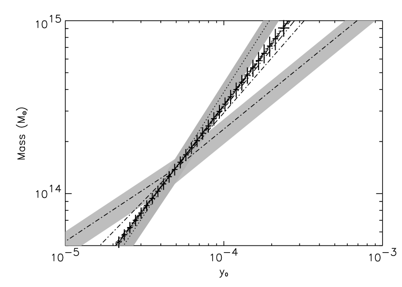
Figure 5.— Cluster physics has a bigger effect on the the scaling of mass with $y_{0}$. This plot shows assorted lines from RS for the mass-$y_{0}$ scaling, with amplitudes normalized to agree at $M=10^{14}\rm M_{\odot}/h$. The crosses show the mass bins and errors for the fiducial model, the RS self-similar phenomenological model, for redshift bin M. The gray regions show the intrinsic scatter in $y_{0}$ according to Motl et al. (2005) for the two most extreme slopes, models 4 (dotted-dashed) and 5 (dotted).

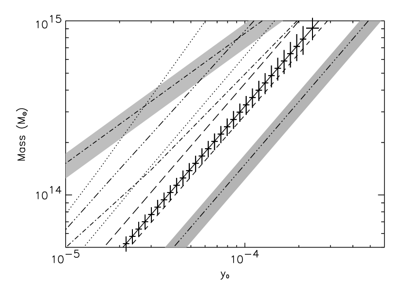
Figure 6.— Assorted models from RS for the mass-$y_{0}$ scaling, with amplitudes not normalized. The crosses show the bins and errors for the fiducial model, the RS self-similar phenomenological model, for redshift bin M. The gray regions show the intrinsic scatter in $y_{0}$ according to Motl et al. (2005) for the two most extreme amplitudes. The dotted-dashed lines show the extreme preheating models, the dotted lines show the extreme polytropic models, the dashed lines show the extreme accretion pressure models, and the triple-dotted dashed lines show the different values for $s_{1}$, the exponent of the radius in the radial profile of $K$.

Taking the RS self-similar model as our fiducial, with a slope $0.84$ and an amplitude $4.92$, we plot the expected bin sizes and mass errors for redshift bin M as crosses on the fiducial line (see figure 5). We show the expected scatter from Motl et al. (2005), who computed the scatter from simulations of about 100 clusters, as a shaded gray region around the extreme models. Note that for a survey of 200 square degrees, one expects to detect about 2000 clusters, so the effect of this scatter on the determination of slope and amplitude of the scaling relation should be reduced. The two RS models with extreme slopes for this scaling are the analytical model with the largest preheating ($K_{\mathrm{preheat}}=5\times 10^{33}$ erg cm² g^-5/3), model 4, and the polytropic model with $\gamma=1.2,\rho_{2}=1.06\rho_{1}$, model 5. We can distinguish model 4’s slope from the fiducial model at more than the $5\sigma$ level for all redshift bins, and can distinguish model 5 quite well in the lower two redshift bins (see table 10).

Figure 6 shows the lines for various RS models without normalized amplitudes. The models with extreme amplitudes are model 4 (the preheating model) and model 6, the model with $s_{1}=1.5$. We can distinguish both models’ amplitudes from the fiducial model at $\gg$ 5 sigma in all redshift bins and we can start constraining the parameters describing cluster physics, e.g., the amount of entropy injection.

Table 10 shows a few RS models, their amplitudes for the $y_{0}-M$ scaling, and their $\sigma$ from the fiducial. Notice we can easily distinguish models with amplitudes that vary by about 20%. Physics that causes such a difference in amplitude includes changing the entropy profile normalization by a factor of 1.5, doubling the radius at which the entropy maxes out, changing the accretion rate by a factor of 3.5, or increasing the exponent $s_{1}$ of the radial entropy profile from 1.1 to 1.5.

As the slope for the $y_{0}$ relation is 0.84 (range 0.71 - 1.5), an additional $x$% systematic error on the mass determination would propagate into an additional $\sim 0.8\times x$% error on the amplitude of the scaling relation. Even allowing for a 10% systematic mass error we find that, for redshift bin M, we can distinguish all of the RS preheating models, polytropic models, $s_{1}=0.7$, and $s_{1}=1.5$, to more than $5\sigma$. We can distinguish the models with varying accretion pressure (models 2 and 3) to more than $2\sigma$. The range of amplitudes $A_{y}$ are $7.0\times 10^{-6}$ to $9.4\times 10^{-5}$ (fiducial $4.9\times 10^{-5}$).

Since the models with maximum and minimum slope and amplitude are different for $y_{0}$ than for $L_{sz}$, combining the two would allow for further distinctions among models of cluster physics.

In the cases where the two parameters fit yields a $S/N>5$ in principle there could be enough S/N to add parameters to the fit, or in other words to investigate if e.g., deviations from a power law in the scaling relation can yield additional information about cluster physics.

Here we have concentrated on a survey with the properties and sky coverage of ACT and its optical follow up. Naturally a wider SZ survey with weak lensing follow up and/or a weak lensing follow up from space will improve these constraints. A space telescope can yield $n_{g}=100$ galaxies per square arcminutes. While for low and intermediate redshift this will improve constraints reported here only by $~{}\sqrt{5}$, as the additional galaxies are likely to have a distribution with a higher-redshift tail, the constraints at the higher redshift will show a better improvement. This may open up the possibility to study redshift evolution of the ICM. On the other hand a ground-based survey covering 1000 square degrees will also yield constraint better by a factor $\sqrt{5}$, providing better discriminative power between models. Finally a combination of ground-based SZ observations over 1000 square degrees with space-based weak lensing follow up would yield improved constraints by a factor 5. This combination is not too dissimilar from the planned SNAP observations if ACT could scan in SZ the same region of the sky.

Cluster model	$\alpha_{M}$
# $\sigma_{\alpha_{M}}$ from fiducial, pessimistic             # $\sigma_{\alpha_{M}}$ from fiducial optimistic
		$z$ bin L	$z$ bin M	$z$ bin H	$z$ bin L	$z$ bin M	$z$ bin H
$K_{\mathrm{ph}}=10^{30}$ (Model 1)	1.77	1.1	2	0.4	1.4	2.6	0.6
$\omega_{\mathrm{accr}}=0.28$ (Model 2)	1.64	0.5	1	0.2	0.7	1.3	0.3

Table 6 Two extreme slope models we consider, described by Reid & Spergel (2005), their best-fit slopes $\alpha_{M}$ (where $L_{sz}=A(M/M_{o})^{\alpha_{M}}$), and the number of $\sigma$ between their slopes and the fiducial slope in the three redshift bins and in both the optimistic and pessimistic cases.

Cluster model	$A$ (kpc2)
# $\sigma_{A}$ from fiducial, pessimistic             # $\sigma_{A}$ from fiducial optimistic
		$z$ bin L	$z$ bin M	$z$ bin H	$z$ bin L	$z$ bin M	$z$ bin H
$K_{\mathrm{ph}}=10^{30}$ (Model 1)	4.76	3	6	1.8	4.5	8	2.3
$\omega_{\mathrm{accr}}=3.5$ (Model 3)	7.78	3	5	1.6	3.9	7	2

Table 7 Two extreme amplitude models we consider, described by Reid & Spergel (2005), their best-fit amplitudes $A$ (where $L_{sz}=A(M/M_{o})^{\alpha_{M}}$), and the number of $\sigma$s between their amplitudes and the fiducial amplitude in the three redshift bins and in both the optimistic and pessimistic cases.

Cluster model	$\alpha_{My}$
# $\sigma_{\alpha_{My}}$ from fiducial, pessimistic         # $\sigma_{\alpha_{My}}$ from fiducial optimistic
		$z$ bin L	$z$ bin M	$z$ bin H	$z$ bin L	$z$ bin M	$z$ bin H
$K_{\mathrm{ph}}=5\times 10^{33}$ (Model 4)	1.50	$>$5	$>$5	$>$5	$>$5	$>$5	$>$5
$\gamma=1.2$, $\rho_{2}=1.06\rho_{1}$ (Model 5)	0.71	2	3	1	3	5	1.2

Table 8Two extreme slope models (for the central Compton parameter) we consider, described by Reid & Spergel (2005), their best-fit slopes $\alpha_{My}$ (where $y_{0}=A_{y}(M/M_{o})^{\alpha_{My}}$), and the number of $\sigma$ between their slopes and the fiducial slope in the three redshift bins and in both the optimistic and pessimistic cases.

Table 9Two extreme slope models (for the central Compton parameter) we consider, described by Reid & Spergel (2005), their best-fit slopes $\alpha_{My}$ (where $y_{0}=A_{y}(M/M_{o})^{\alpha_{My}}$), and the number of $\sigma$ between their slopes and the fiducial slope in the three redshift bins and in both the optimistic and pessimistic cases.

Cluster model	$A_{y}$ ($10^{-5})$
# $\sigma_{A_{y}}$ from fiducial, pessimistic         # $\sigma_{A_{y}}$ from fiducial optimistic
		$z$ bin L	$z$ bin M	$z$ bin H	$z$ bin L	$z$ bin M	$z$ bin H
$K_{\mathrm{max}}=K_{200}$ (Model 7)	5.66	2.9	4.4	1.9	3.2	4.7	2.2
$K_{\mathrm{max}}=1.5K_{100}$ (Model 8)	3.84	5	$>$6	3.4	5.6	$>$6	4
$\omega_{\mathrm{accr}}=0.28$ (Model 2)	5.41	1.9	3	1.3	2.1	3.1	1.5
$\omega_{\mathrm{accr}}=3.5$ (Model 3)	4.33	2.7	4	1.8	2.9	4.3	2
$K_{\mathrm{ph}}=5\times 10^{33}$ (Model 4)	0.70	$>$6	$>$6	$>$6	$>$6	$>$6	$>$6
$s_{1}=s_{2}=1.5$ (Model 6)	9.39	$>$6	$>$6	$>$6	$>$6	$>$6	$>$6

Table 10Sample models for the central Compton parameter that fall within 2-6 $\sigma$ from the fiducial in amplitude, described by Reid & Spergel (2005), their best-fit amplitudes $A_{y}$ (where $y_{0}=A_{y}(M/M_{o})^{\alpha_{My}}$), and the number of $\sigma$ between their amplitudes and the fiducial amplitude in the redshift bins and in both the optimistic and pessimistic cases.

4. Discussion and Conclusions

We have shown how, stacking the weak lensing signals from multiple clusters with roughly the same SZ luminosity, the SZ luminosity-mass ($L_{sz}-M$) and SZ central decrement-mass ($y_{o}-M$) relations can be measured from forthcoming SZ surveys with extensive optical follow up. For example, from a survey of 200 square degrees such as ACT, we find we should be able to determine the scaling slope to $\pm 0.05-0.2$ and amplitude to 5-20% depending on redshift bin. Observations indicate that the entropy of the gas in clusters cannot be explained by gravitational collapse alone, but the cause of the increased entropy remains to be determined. Different non-gravitational processes affect both the slope and amplitude of these relations, and in particular the $y_{o}-M$ relation is most sensitive to cluster physics. Used in conjunction with results from simulations, the expected errors on the measurements of the slope and amplitude of scaling relations imply that we can start to discriminate among different non-gravitational processes affecting the ICM.

We have shown that, for a survey of $\sim$ 200 sq. deg., the available S/N enables one to measure these scaling relations as a function of redshift: we can distinguish slopes and amplitudes of the $M-L_{sz}$ relation and $M-y_{0}$ relation for different redshift bins with width $\Delta z=\pm 0.1$, thus opening up the possibility to constrain how the mass-SZ scaling evolves with redshift. A mass measurement from weak lensing and a SZ measurement in different redshift bins, can constrain the evolution of hot gas as a function of redshift, which in turn would enable one to constrain feedback evolution. Inspection of Fig. 3 and 4 provides a quantitative measurement of how physics in clusters, e.g. feedback, can be constrained as a function of redshift. The errors reported here will scale with the survey parameters as $1/\sqrt{f_{\rm sky}}$ and $1/\sqrt{n_{g}}$. Thus, using this method, wider surveys can improve constraints on cluster physics just as well as deeper surveys. For a space telescope with $n_{g}=100$ galaxies per square arcminute and 1000 square degrees, our results would improve by a factor of 5.

A calibration of the SZ-Mass relation with known uncertainties also has consequences for the determination of cosmological parameters. The number density of clusters within a given mass range or above a given mass is extremely sensitive to cosmology. This sensitivity, in principle, can lead to tight constraints on cosmological parameters such as $\Omega_{m}$, dark energy properties and neutrino mass. However, even relatively small systematic errors in clusters mass estimates can lead to systematic errors on the recovered cosmological parameters that are larger than the statistical ones (Holder et al., 2001; Battye & Weller, 2003; Francis et al., 2005). This potentially compromises measurements of parameters like e.g. the dark energy equation of state. The technique outlined in this paper to calibrate the mass-SZ relation may help reduce the amplitude of these systematic errors. The weak lensing mass determination used here is sensitive to the mass along the line of sight, not just the gas. It is true that there can be biases introduced by the large-scale structure local to the clusters, but we argue that this should not be considered a fundamental limitation as this effect in principle can be quantified by means of numerical N-body simulations. If this can be achieved, our estimates above indicate that the residual uncertainty in the calibration of the amplitude of the mass-SZ relation is $~{}5$% for a survey with $n_{g}=20$ galaxies per square arcminute and sky coverage of 200 square degrees. This uncertainty would propagate into a systematic error in the determination of cosmological parameters, that is now reduced to be not larger than the statistical uncertainty achievable from a survey of the same size (see Francis et al. (2005)). Alternatively, The M-L_SZ relation calibrated in this way from a small area of the sky can be used to determine masses of SZ clusters from very large SZ-only surveys, or the $M-y_{0}$ relation could be used to constrain cluster physics and this information can then be used to model the $M-L_{sz}$ relation. This approach is nicely complementary to other techniques proposed to calibrate the mass-observable relations such as the self-calibration using the cluster power spectrum of Majumdar & Mohr (2004). While only positions and redshifts of clusters are needed to measure the power spectrum and thus to self-calibrate the SZ-Mass relation, it requires observations of large areas of the sky as square and contiguous as possible. The calibration of the M-SZ relation with weak lensing has more stringent follow up requirements (imaging with good seeing in addition to clusters redshifts), but has less stringent geometry requirements.

References

- Bartelmann & Schneider (2001) Bartelmann, M., & Schneider, P. 2001, Phys. Rep., 340, 291
- Battye & Weller (2003) Battye, R. A., & Weller, J. 2003, Phys. Rev., D68, 083506
- Bryan & Norman (1998) Bryan, G. L., & Norman, M. L. 1998, Astrophys. J., 495, 80
- Bullock et al. (2001) Bullock, J. S., et al. 2001, Mon. Not. Roy. Astron. Soc., 321, 559
- Cen (1997) Cen, R. 1997, ApJ, 485, 39
- Clowe et al. (2004) Clowe, D., Gonzalez, A., & Markevitch, M. 2004, Astrophys. J., 604, 596
- Clowe et al. (2005) Clowe, D., et al. 2005, astro-ph/0511746
- da Silva et al. (2004) da Silva, A. C., Kay, S. T., Liddle, A. R., & Thomas, P. A. 2004, Mon. Not. Roy. Astron. Soc., 348, 1401
- Dodelson (2004) Dodelson, S. 2004, Phys. Rev., D70, 023008
- Dos Santos & Dore (2001) Dos Santos, S., & Dore, O. 2001, astro-ph/0106456
- Eisenstein & Hu (1997) Eisenstein, D. J., & Hu, W. 1997, Astrophys. J., 511, 5
- Francis et al. (2005) Francis, M. R., Bean, R., & Kosowsky, A. 2005, astro-ph/0511161
- Hoekstra (2001) Hoekstra, H. 2001, A&A, 370, 743
- Hoekstra (2003) Hoekstra, H. 2003, Mon. Not. Roy. Astron. Soc., 339, 1155
- Holder et al. (2001) Holder, G., Haiman, Z., & Mohr, J. 2001, Astrophys. J., 560, L111
- Kaiser & Squires (1993) Kaiser, N., & Squires, G. 1993, Astrophys. J., 404, 441
- Lapi et al. (2005) Lapi, A., Cavaliere, A., & Menci, N. 2005, Astrophys. J., 619, 60
- Majumdar & Mohr (2004) Majumdar, S., & Mohr, J. J. 2004, ApJ, 613, 41
- Marian & Bernstein (2005) Marian, L., & Bernstein, G. 2005, in preparation
- McCarthy et al. (2003) McCarthy, I. G., Babul, A., Holder, G. P., & Balogh, M. L. 2003, Astrophys. J., 591, 515
- McCarthy et al. (2003) McCarthy, I. G., Babul, A., Holder, G. P., & Balogh, M. L. 2003, ApJ, 591, 515
- Metzler et al. (1999) Metzler, C. A., White, M. J., Norman, M., & Loken, C. 1999, Astrophys. J., 520, L9
- Motl et al. (2005) Motl, P. M., Hallman, E. J., Burns, J. O., & Norman, M. L. 2005, Astrophys. J., 623, L63
- Nagai (2005) Nagai, D. 2005, astro-ph/0512208
- Navarro et al. (1997) Navarro, J. F., Frenk, C. S., & White, S. D. M. 1997, Astrophys. J., 490, 493
- Oh & Benson (2003) Oh, S. P., & Benson, A. J. 2003, Mon. Not. Roy. Astron. Soc., 342, 664
- Ostriker et al. (2005) Ostriker, J. P., Bode, P., & Babul, A. 2005, Astrophys. J., 634, 964
- Reid & Spergel (2005) Reid, B. A., & Spergel, D. N. 2005, in preparation
- Roychowdhury et al. (2005) Roychowdhury, S., Ruszkowski, M., & Nath, B. B. 2005, astro-ph/0508120
- Sheldon et al. (2001) Sheldon, E. S., et al. 2001, Astrophys. J., 554, 881
- Sheth & Tormen (1999) Sheth, R. K., & Tormen, G. 1999, Mon. Not. Roy. Astron. Soc., 308, 119
- Spergel et al. (2003) Spergel, D. N., Verde, L., Peiris, H. V., Komatsu, E., Nolta, M. R., Bennett, C. L., Halpern, M., Hinshaw, G., Jarosik, N., Kogut, A., Limon, M., Meyer, S. S., Page, L., Tucker, G. S., Weiland, J. L., Wollack, E., & Wright, E. L. 2003, APJS, 148, 175
- Sunyaev & Zeldovich (1980) Sunyaev, R. A., & Zeldovich, Y. B. 1980, ARAA, 18, 537
- White et al. (2002) White, M. J., Hernquist, L., & Springel, V. 2002, Astrophys. J., 579, 16
- Wright & Brainerd (2000) Wright, C. O., & Brainerd, T. G. 2000, ApJ, 534, 34