News from the “Dentist’s Chair”: Observations of AM 1353-272 with the VIMOS IFU

Abstract

The galaxy pair AM 1353-272 nicknamed “The Dentist’s Chair” shows two $\sim$30 kpc long tidal tails. Previous observations using multi-slit masks showed that they host up to seven tidal dwarf galaxies. The kinematics of these tidal dwarfs appeared to be decoupled from the surrounding tidal material. New observations of the tip of the southern tidal tail with the VIMOS integral field unit confirm the results for two of these genuine tidal dwarfs but raise doubts whether the velocity gradient attributed to the outermost tidal dwarf candidate is real. We also discuss possible effects to explain the observational difference of the strongest velocity gradient seen in the slit data which is undetected in the new integral field data, but arrive at no firm conclusion. Additionally, low-resolution data covering most of the two interacting partners show that the strongest line emitting regions of this system are the central parts.

1 Introduction

Following old ideas about the creation of dwarf galaxies during interaction of giant galaxies and detailed investigations of several nearby examples of these Tidal Dwarf Galaxies (TDGs, Duc et al., 2000, 1997; Duc & Mirabel, 1998; Hibbard et al., 1994), we carried out a first small survey of interacting galaxies (Weilbacher et al., 2000) with the aim of better understanding the star-formation history of TDGs and constraining the number of TDGs that are built per interaction (Weilbacher et al., 2003). During this survey, we studied a system cataloged as AM 1353-272, which we called “The Dentist’s Chair” for its peculiar shape. Fig. 1 shows the two components of the system, ‘A’, a galaxy with $\sim$30 kpc long tidal tails, and ‘B’, a disturbed disk galaxy, have a distance of $D\approx 160$ Mpc ($H_{0}=75$ km s^-1 Mpc^-1). Within the tails several obvious clumps with blue optical colors are visible. Using optical and near-infrared imaging, evolutionary models, and optical spectroscopy, seven of these clumps were classified as TDG candidates in formation (Weilbacher et al., 2002, , marked ‘a’ to ‘d’ and ‘k’ to ‘m’). The largest velocity gradient with an amplitude of $>$300 km s^-1 appeared in TDG candidate ‘a’, at the very end of the southern tidal tail. This raised the question how an object with relatively low luminosity could exhibit such fast “rotation”. However, as these observations were done using the multi-slit technique and hence are spatially restricted due to the narrow slit, subsequent observations were planned using an integral field unit (IFU) to cover more of the tidal tails and view the velocity structure of the TDGs in two dimensions.

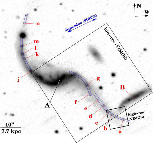
Figure 1: The interacting system AM 1353-272. The two interacting galaxies (capital letters) and the relevant knots in the tidal tails are marked (lower case letters). Overlayed are the original FORS2 slits and the two VIMOS pointings in low and high resolution mode.

2 IFU Observations

Our new VIMOS data taken at the ESO VLT consists of 1.3 hours of exposure time in high resolution blue mode (field of view of 13^′′$\times$13^′′) and good seeing conditions ($\sim$0$.\!\!^{\prime\prime}$7), targeted at the tip of the southern tidal tail. This includes the TDG candidates ‘a’ to ‘c’. The center of galaxy ‘A’, much of the southern tidal tail, and the companion ‘B’ were targeted with low-resolution (blue grism, 54^′′$\times$54^′′), and observed for 1 hour in mediocre conditions with $\sim$2$.\!\!^{\prime\prime}$0 seeing. These two pointings are sketched in Fig. 1.

The data were reduced using the ESO pipeline for the VIMOS instrument. We made a small enhancement to the code that allowed us to interpolate the wavelength solution between adjacent spectra on the CCD. This was only used for the low-resolution data, where the errors introduced with this method are smaller than the accuracy allowed for by the spectral resolution. In low-resolution mode, on the order of 15% of the spectra could not be wavelength calibrated due to overlapping spectral orders. From the final datacube of extracted and wavelength calibrated spectra, we measured the relative fluxes and velocities in each spectral element using Gaussian fits to the brightest usable emission line. In the low-resolution data [Oiii]5007 is the strongest emission line but at this redshift ($z\approx 0.04$) it is strongly blended with a sky emission line, so H$\beta$ had to be used instead. In the high-resolution data, [Oiii]5007 is less affected by the sky-line and is the only line with sufficient S/N for the analysis in the low surface brightness region near the end of the tidal tail.

3 Results

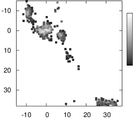
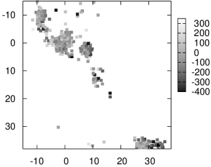
Figure 2: Results of the low-resolution pointing, the center of AM 1353-272 A is at the coordinates (0,0); at the bottom right, near (30,32) companion ‘B’ is visible. Axes labels are in arcseconds. Left: relative H$\beta$ emission line flux (bright: high flux, dark: low flux). Right: velocity field derived from H$\beta$ emission line (the greyscale bar gives relative velocities in km s^-1).

Fig. 2 summarizes the results that can be derived from the low-resolution pointing using fits to the H$\beta$ emission line. The southern tidal tail in undetected in this exposure and the strongest line emission appears to be in the center of ‘A’ and in the two knots at the end of its bar-like central structure (designated ‘g’ and ‘j’ in Weilbacher et al., 2002). Galaxy ‘B’, despite being strongly reddened, also is a strong source of H$\beta$ line emission. As the velocity resolution is on the order of 100 km s^-1, in this mode of VIMOS we cannot resolve the velocity structures in individual knots, but the bar-like structure in ‘A’ seems to rotate (the eastern end near knot ‘j’ is receding, the western end near knot ‘g’ is approaching). The same is true for the companion ‘B’.

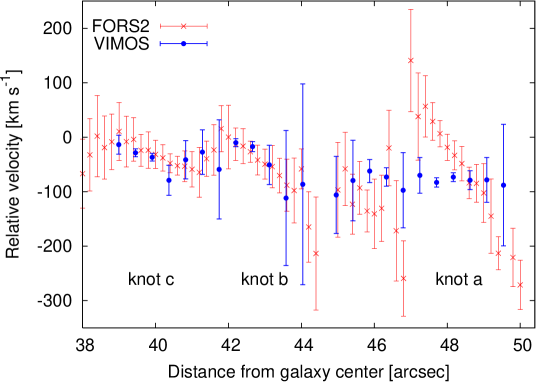
Figure 3: Velocity field as derived from FORS2 observations (black points) and reconstruction of this velocity field from the VIMOS IFU datacube (grey crosses).

To verify our original FORS2 multi-slit observations, we try to “reconstruct” them from the VIMOS datacube. To that end we average over the spaxels approximately in the dispersion direction of the FORS2 observations and derive an average redshift over the slit width. Fig. 3 shows the resulting velocity field along this artificial slit and compares it with the velocity profile of the FORS2 data. From this plot it can be seen that the velocity gradients of knots ‘b’ and ‘c’ are very well recovered, while the steep slope within knot ‘a’ with an amplitude of $\sim$350 km s^-1 in the FORS2 data appears almost flat in the reconstructed VIMOS data. We tested several alternative slit positions and curvatures, varied the effective slit width, and also tried to add slit effects (velocity offsets due to non-centered emission within the slit) to our reconstruction. None of these changes improved the match for knot ‘a’. In fact, slit effects significantly worsened the agreement for all three knots. The FORS2 observations were done on these extended objects in 1$.\!\!^{\prime\prime}$0 seeing with a 1$.\!\!^{\prime\prime}$2 slit, so that it appears unlikely that slit effects would have a strong contribution to the observed velocity gradient. Other problems, like instrumental flexures should have been removed by the data reduction procedure as detailed in Weilbacher et al. (2002). We are therefore confident that slit effects do not play an important role in the FORS2 data. On the other hand, if we assume that the original slit-based data give the correct results it is unclear, how the VIMOS data could be flawed to hide this one velocity gradient. The wavelength calibration works well for the high-resolution mode as confirmed by checks with sky emission lines.

4 Summary & Outlook

We presented a few tentative results for the interacting system called “The Dentist’s Chair” from new observations with the VIMOS integral field mode: line emission seems to be concentrated within the centers of the interacting partners while the tidal tails themselves are not detected H$\beta$ narrowband slices. Three knots, previously identified as TDG candidates near the end of the southern tidal tail, are detected in [Oiii]5007 emission. For two of them the velocity profiles were confirmed. However, the strongest velocity gradient in the outermost TDG candidate (knot ‘a’) as measured on FORS2 data is not confirmed by the VIMOS datacube. The reason for this discrepancy is unknown.

To solve this mystery and find more clues to the origin of the velocity fields seen in this interacting system, further, deeper IFU observations, taken with appropriate dither offsets to facilitate more accurate sky subtraction, are required. With other instruments like e. g. the GMOS IFU would be possible to cover both the Ca-triplet and H$\alpha$ in the same exposures and directly compare the stellar velocity field with ionized gas dynamics. As good S/N is required to detect the absorption lines, this can only be done in the brighter northern tidal tail.