Turbulence, magnetic fields and plasma physics in clusters of galaxies

Abstract

Observations of galaxy clusters show that the intracluster medium (ICM) is likely to be turbulent and is certainly magnetized. The properties of this magnetized turbulence are determined both by fundamental nonlinear magnetohydrodynamic interactions and by the plasma physics of the ICM, which has very low collisionality. Cluster plasma threaded by weak magnetic fields is subject to firehose and mirror instabilities. These saturate and produce fluctuations at the ion gyroscale, which can scatter particles, increasing the effective collision rate and, therefore, the effective Reynolds number of the ICM. A simple way to model this effect is proposed. The model yields a self-accelerating fluctuation dynamo whereby the field grows explosively fast, reaching the observed, dynamically important, field strength in a fraction of the cluster lifetime independent of the exact strength of the seed field. It is suggested that the saturated state of the cluster turbulence is a combination of the conventional isotropic magnetohydrodynamic turbulence, characterized by folded, direction-reversing magnetic fields and an Alfvén-wave cascade at collisionless scales. An argument is proposed to constrain the reversal scale of the folded field. The picture that emerges appears to be in qualitative agreement with observations of magnetic fields in clusters.

I Introduction

Clusters of galaxies are vast and varied objects that have long attracted the attention of both observers (in recent decades spectacularly aided by X-ray and radio telescopes) and theoreticians. The observed properties of clusters have proved far from easy to explain as new data has confounded many old theories.

The overall budget of the cluster constituents is roughly as follows: $\sim 75\%$ of cluster mass is dark matter, whose sole function is assumed to be to provide the gravitational well, $\sim 20\%$ of cluster mass is the diffuse X-ray-emitting plasma (the intracluster medium, or ICM), while the galaxies have an all but negligible mass. The plasma that makes up the ICM is made of hot and tenuous ionized hydrogen: temperatures are in the range of $1-10$ keV, number densities $\sim 10^{-1}-10^{-3}~{}\text{cm}^{-3}$, with colder, denser material found in the cool cores and hotter, more diffuse one in the outlying regions.

Necessarily, the first observations and the first theoretical models of clusters concerned what one might call large-scale features, such as the overall profiles of mass and temperature, the structure formation and the role of the central objects. As observations increased in accuracy and resolution, the ICM was revealed to be much richer than simply a dull cloud of X-ray glow smoothly petering out with distance from the center. A great panoply of features has been detected: bubbles, filaments, ripples, edges, shocks, sound waves, etc., as well as very chaotic density, temperature and abundance distributions.Fabian et al. (2003a, 2006, 2005); Schuecker et al. (2004); Churazov et al. (2003) It is particularly the presence of chaotic fields and the evidence that this chaos exists in a range of scalesSchuecker et al. (2004); Vogt and Enßlin (2003, 2005) that makes one expect that ICM, like so many other astrophysical plasmas, is in a turbulent state. It is essential to know the properties of this turbulence in order to predict the current and future statistical measurements of the plasma and magnetic fields (spectra, correlation and distribution functions, etc.) and to model correctly the transport processes in the ICM that determine, for example, the overall temperature profiles.Voigt and Fabian (2004); Dennis and Chandran (2005)

We shall assume that the physics of small scales is, at least to some degree, independent of large-scale circumstances and that we can, therefore, gain some useful understanding of the turbulence in clusters by ignoring large-scale features and considering a homogeneous subvolume of the ICM. In what follows, after reviewing briefly what is known about fluid motions (Sec. II) and magnetic fields (Sec. III) in clusters, we describe, mostly in qualitative terms, what we consider to be the essential aspects of the small-scale physics of the ICM (for plasma physics, see Sec. IV). This will lead us to a tentative overall picture of the structure of the ICM turbulence (Sec. VI) as well as of the origin of its magnetic component (Sec. V). We must emphasize that the current state of the debates on the nature of turbulence in clusters (and, indeed, on its very existenceFabian et al. (2003b)) is such that even a fundamental, conceptual view of the problem has not yet been agreed, and, therefore, a quantitative theory — even an incomplete one such as exists for hydrodynamic turbulence — remains a matter of future work.

II Turbulence

The failure of one of the instruments on the ASTRO-E2 satellite has set off the planned direct detection of cluster turbulenceSunyaev et al. (2003); Inogamov and Sunyaev (2003) into the (probably not very distant) future. However, indirect evidence of turbulent gas motions does exist: three recent examples are the broad spectrum of pressure fluctuations measured in the Coma clusterSchuecker et al. (2004), detection of subsonic gas motions in the core of the Perseus cluster,Churazov et al. (2004) and, again for the Perseus cluster, the broadening (assumed to be caused by turbulent diffusion) of abundance peaks associated with the brightest cluster galaxies.Rebusco et al. (2005) These and other studies and models based on observational data appear to converge in expecting turbulent flows with rms velocities in the range $U\sim 10^{2}-10^{3}$ km/s at the outer scales $L\sim 10^{2}$ kpc. The energy sources for this turbulence are probably the cluster and subcluster merger events and/or, especially for the turbulence in cool cores, the active galactic nuclei (AGN). The aforementioned observational estimates of the strength and scale of the turbulence are in order-of-magnitude agreement with the outcomes of numerical simulations of cluster formationNorman and Bryan (1999); Sunyaev et al. (2003); Ricker and Sarazin (2001) and of the buoyant rise of radio bubbles generated by the AGN.Churazov et al. (2001); Fujita (2005) Further discussion and references on the stirring mechanisms for cluster turbulence can be found in Refs. Subramanian et al., 2006, Enßlin and Vogt, 2006, Chandran, 2005.

Table 1: Cluster Parameters

Parameter	Expression	Cool cores	Hot ICM
$T$	observed	$3\times 10^{7}$ K	$10^{8}$ K
$n$	observed	$6\times 10^{-2}~{}\text{cm}^{-3}$	$10^{-3}~{}\text{cm}^{-3}$
$v_{\text{th},i}$	$(2T/m_{i})^{1/2}$	$700$ km/s	$1300$ km/s
$\nu_{ii}$	$1.5\,nT^{-3/2}$	$5\times 10^{-13}~{}\text{s}^{-1}$	$2\times 10^{-15}~{}\text{s}^{-1}$
$\lambda_{\text{mfp}}$	$v_{\text{th},i}/\nu_{ii}$	$0.05$ kpc	$30$ kpc
$\mu_{\parallel}$	$v_{\text{th},i}\lambda_{\text{mfp}}$	$10^{28}~{}\text{cm}^{2}$/s	$10^{31}~{}\text{cm}^{2}$/s
$\eta$	$3\times 10^{13}T^{-3/2}$	$200~{}\text{cm}^{2}$/s	$30~{}\text{cm}^{2}$/s
$U$	inferred	$250$ km/s	$300$ km/s
$L$	inferred	$10$ kpc	$200$ kpc
$L/U$	inferred	$4\times 10^{7}$ yr	$7\times 10^{8}$ yr
Re	$UL/\mu_{\parallel}$	$70$	$2$
Rm	$UL/\eta$	$4\times 10^{27}$	$6\times 10^{29}$
$t_{\text{visc}}$	$(L/U)\text{Re}^{-1/2}$	$5\times 10^{6}$ yr	$5\times 10^{8}$ yr
$l_{\text{visc}}$	$L\text{Re}^{-3/4}$	$0.4$ kpc	$100$ kpc
$l_{\text{res}}$	$L\text{Rm}^{-1/2}$	$5000$ km	$8000$ km
$\Omega_{i,\text{eq}}$	$eB_{\text{eq}}/cm_{i}$	$0.3~{}\text{s}^{-1}$	$0.04~{}\text{s}^{-1}$
$\rho_{i,\text{eq}}$	$v_{\text{th},i}/\Omega_{i,\text{eq}}$	$3000$ km	$30,000$ km
$B_{0}$	$B_{\text{eq}}\rho_{i,\text{eq}}/\lambda_{\text{mfp}}$	$5\times 10^{-17}$ G	$2\times 10^{-19}$ G
$B_{1}$	Eq. (13)	$3\times 10^{-14}$ G	$2\times 10^{-17}$ G
$B_{2}$	Eq. (15)	$8\times 10^{-7}$ G	$2\times 10^{-7}$ G
$B_{\text{visc}}$	$B_{\text{eq}}\text{Re}^{-1/4}$	$9\times 10^{-6}$ G	$4\times 10^{-6}$ G
$B_{\text{eq}}$	$(8\pi m_{i}nU^{2}/2)^{1/2}$	$3\times 10^{-5}$ G	$4\times 10^{-6}$ G
$\beta_{\text{eq}}$	$8\pi nT/B_{\text{eq}}^{2}$	$8$	$20$
$l_{\perp}$	$(B_{2}/B_{\text{eq}})L$	$0.2$ kpc	$7$ kpc
$l_{B}$	observed	$1$ kpc	$10$ kpc

While estimates of the turbulence parameters appear robust roughly to within an order of magnitude, a more quantitative set of numbers is elusive, partly because of the indirect and difficult nature of the observations, partly because the conditions vary both in different clusters and within each individual cluster. Here we shall adopt two fiducial sets of parameters: one for cool cores and one for the bulk of hot cluster plasma. These are given in Table 1 (along with some theoretical quantities that will arise in Sec. V and Sec. VI). They will allow us to make estimates that will have the virtue of being consistent and systematic but must not be interpreted as precise quantitative predictions. They are representative of the range of conditions that can be present in clusters. The turbulence is assumed to be stirred at the outer scale $L$ (with rms velocity $U$ at this scale) and to have a Kolmogrov-type cascade below this scale. The small-scale cutoff is determined by the microphysical properties of the cluster plasma. In Table 1, we give the value of the particle mean free path $\lambda_{\text{mfp}}$, which can be used in a naive estimate of viscosity: $\mu_{\text{ICM}}\sim v_{\text{th},i}\lambda_{\text{mfp}}$, where $v_{\text{th},i}=(2T/m_{i})^{1/2}$ is the ion thermal speed. We see that this gives fairly low values for the Reynolds number, $\text{Re}\sim UL/\mu_{\text{ICM}}$. It is this feature of the ICM that continues to fuel doubts about its ability to support turbulence, at least in the strict, hydrodynamic high-Reynolds-number sense. However, one should be cognizant of the fact that whatever type of turbulence might exist in the cluster plasma, it is certainly not hydrodynamic, because this plasma is highly electrically conducting and magnetized. The presence of the magnetic fields not only has a dynamical effect on the turbulence (due to the action of the Lorentz force, the medium acquires a certain elastic quality), but also changes the transport properties of the plasma itself: the viscosity, in particular, becomes strongly anisotropic.Braginskii (1965) These issues will constitute the main subject of this paper, but first let us briefly describe what is known about magnetic fields in clusters.

III Magnetic fields

The first observed signature of cluster magnetic fields was the diffuse synchrotron radio emission in the Coma cluster detected in 1970.Willson (1970) Starting from early 1990’s, increasingly detailed measurements of the Faraday Rotation in the emission from intracluster radio sources have made possible quantitative estimates of the magnetic field strength and scales in a large number of clusters.Kronberg (1994); Carilli and Taylor (2002); Govoni and Feretti (2004) Randomly tangled magnetic fields with rms strength of order $B_{\text{rms}}\sim 1-10~{}\mu$G are consistently found, with the fields in the cool cores of the cooling-flow clusters somewhat stronger than elsewhere. This is fairly close to the value $B_{\text{eq}}$ that corresponds to magnetic energy equal to the energy of turbulent motions (see Table 1). Thus, the magnetic field must be dynamically important. The estimates for the tangling scale $l_{B}$ of the field are usually arrived at by assuming that direction reversals along the line of sight (probed by the Faraday Rotation measure) can be described as a random walk with a single step size equal to $l_{B}$ (the estimate of $B_{\text{rms}}$ is obtained in conjunction with this model). This gives $l_{B}\sim 1-10$ kpc.

The single-scale model is almost certainly not a correct description on any but a very rough level. Fortunately, much more detailed information on the spatial structure of the cluster fields is accessible. First, using certain statistical assumptions (most importantly, isotropy), it is possible to compute magnetic-energy spectra from the maps of the Faraday Rotation measure associated with extended radio sources (the radio lobes of the jets emerging from the AGN — these can be as large as $\sim 10^{2}$ kpc across).Enßlin and Vogt (2003); Vogt and Enßlin (2003) This has been done most thoroughly for a radio lobe located in the cool core of the Hydra A cluster.Vogt and Enßlin (2005) The spectrum has a peak at $k\simeq 2~{}\text{kpc}^{-1}$ followed by what appears to be a power tail consistent with $k^{-5/3}$ down to the resolution limit of $k\simeq 10~{}\text{kpc}^{-1}$. The rms magnetic field strength is $B_{\text{rms}}=7\pm 2~{}\mu$G.

The second source of information on the cluster field structure is the polarized synchrotron emission, which probes the magnetic field in the plane perpendicular to the line of sight.Burn (1966) Such data, while widely used for Galactic magnetic field studies,Haverkorn et al. (2003) has until recently not been available for clusters. This is now changing: the first analysis of polarized emission from a radio relic in the cluster A2256 reveals the presence of magnetic filaments with field reversals probably on $\sim 20$ kpc scale, which, however, is dangerously close to the resolution scale.Clarke and Enßlin (2006) This data is representative of the situation in the bulk of the ICM, rather than in the cores. Statistical analysis of such data will make possible quantitative diagnosis of the field structure and its dynamical role.Enßlin et al. (2006)

Thus, our knowledge of the magnetic fields in clusters, while far from perfect, is more direct and more detailed than that of the turbulent motions of the ICM. It is also due to improve dramatically with the arrival of new radio telescopes such as LOFAR and SKA.

IV Plasma physics

The key property of the ICM as plasma is that it is only weakly collisional and magnetized: given the observed values of the magnetic field, the ion gyroradius is $\rho_{i}\sim 10^{4}$ km, which is much smaller than the mean free path. As $\rho_{i}\ll\lambda_{\text{mfp}}$ already for dynamically very weak fields ($B\gg B_{0}$, see Table 1), this is true both in the observed present state of the ICM and during most of its hypothetical past, when the magnetic field was being amplified from some weak seed value. In a plasma with $\rho_{i}\ll\lambda_{\text{mfp}}$, the equations for the flow velocity ${\bf u}$ and for the magnetic field ${\bf B}$ may be written in the following form, valid at time scales $\gg\Omega_{i}^{-1}$ ($\Omega_{i}=eB/m_{i}c$ is the ion cyclotron frequency) and spatial scales $\gg\rho_{i}=v_{\text{th},i}/\Omega_{i}$,

$$\rho\,{d{\bf u}\over dt}\!\! = \!\!-\bm{\nabla}\!\left(p_{\perp}+{B^{2}\over 2}\right)+\bm{\nabla}\!\!\cdot\!\left[{\bf\hat{b}}{\bf\hat{b}}\left(p_{\perp}-p_{\parallel}+B^{2}\right)\right],\$$ (1)

$${d{\bf B}\over dt}\!\! = \!\!{\bf B}\cdot\!\bm{\nabla}{\bf u}-{\bf B}\bm{\nabla}\cdot{\bf u},$$ (2)

where $d/dt=\partial/\partial t+{\bf u}\cdot\bm{\nabla}$ is the convective derivative, $p_{\perp}$ and $p_{\parallel}$ are plasma pressures perpendicular and parallel to the local direction of the magnetic field ${\bf B}$, respectively, ${\bf\hat{b}}={\bf B}/B$, the factor of $1/\sqrt{4\pi}$ has been absorbed into ${\bf B}$, and the resistive term has been omitted in Eq. (2) in view of the tiny value of the resistivity. The turbulent motions in clusters are subsonic ($U<v_{\text{th},i}$), so we may take $\bm{\nabla}\cdot{\bf u}=0$ and set $\rho=1$. The magnetic field is, thus, in units of velocity, pressure in units of velocity squared.

The proper way to compute $p_{\perp}$ and $p_{\parallel}$ is by a kinetic calculation. In the collisional limit, this was done in Braginskii’s classic paper.Braginskii (1965) It is instructive to obtain his result in the following heuristic way that highlights the physics behind the formalism.Schekochihin et al. (2005) Charged particles moving in a magnetic field conserve their first adiabatic invariant $\mu=m_{i}v_{\perp}^{2}/2B$. When $\lambda_{\text{mfp}}\gg\rho_{i}$, this conservation is only weakly broken by collisions. As long as $\mu$ is conserved, any change in the field strength causes a proportional change in $p_{\perp}$: summing up the first adiabatic invariants of all particles, we get $p_{\perp}/B=\text{const}$. Then

$${1\over p_{\perp}}{dp_{\perp}\over dt}\sim{1\over B}{dB\over dt}-\nu_{ii}\,{p_{\perp}-p_{\parallel}\over p_{\perp}},$$ (3)

where the second term on the right-hand sight represents the relaxation of the pressure anisotropy at the ion collision rate $\nu_{ii}\sim v_{\text{th},i}/\lambda_{\text{mfp}}$. Using Eq. (2) with $\bm{\nabla}\cdot{\bf u}=0$ and balancing the terms in the rhs of Eq. (3), we get

$$p_{\perp}-p_{\parallel}\sim\mu_{\parallel}\,{1\over B}{dB\over dt}=\mu_{\parallel}{\bf\hat{b}}{\bf\hat{b}}:\bm{\nabla}{\bf u},$$ (4)

where $\mu_{\parallel}\sim p_{\perp}/\nu_{ii}\sim v_{\text{th},i}\lambda_{\text{mfp}}$ is the “parallel viscosity.” Equation (4) turns out to be quantitatively correct provided the value of $\mu_{\parallel}$ with the correct prefactor calculated by BraginskiiBraginskii (1965) is used. Thus, the emergence of the pressure anisotropy is a natural consequence of the changes in the magnetic-field strength and vice versa.

The energy conservation law based on Eqs. (1–2) with $\bm{\nabla}\cdot{\bf u}=0$ and on Eq. (4) is

$${d\over dt}\left({\langle u^{2}\rangle\over 2}+{\langle B^{2}\rangle\over 2}\right) = -\mu_{\parallel}\bigl{<}|{\bf\hat{b}}{\bf\hat{b}}:\bm{\nabla}{\bf u}|^{2}\bigr{>}$$ (5)

$$= -\mu_{\parallel}\left<\left({1\over B}{dB\over dt}\right)^{2}\right>.$$

Thus, the Braginskii viscosity only dissipates such motions that change the strength of the magnetic field. Motions that do not affect $B$ are allowed at subviscous scales. In the weak-field regime, these motions take the form of plasma instabilities. When the magnetic field is strong, a cascade of Alfvén waves can be set up below the viscous scale. Let us elaborate.

The simplest way to see that pressure anisotropies lead to instabilities is as follows.Schekochihin et al. (2005) Imagine that the large-scale energy sources stir up a “fluid” turbulence with ${\bf u}$, $p_{\perp}$, $p_{\parallel}$, ${\bf B}$ at time and spatial scales above viscous. Would such a solution be stable with respect to much higher-frequency and smaller-scale perturbations? Linearizing Eq. (1) and denoting perturbations by $\delta$, we get

$$\!\!\!\!-i\omega\delta{\bf u}\!\! = \!\!-i{\bf k}\left(\delta p_{\perp}+B\delta B\right)+\left(p_{\perp}-p_{\parallel}+B^{2}\right)\delta{\bf K}$$ (6)

$$\!\!+\,\,i{\bf\hat{b}}\,k_{\parallel}\!\left[\delta p_{\perp}-\delta p_{\parallel}-\left(p_{\perp}-p_{\parallel}-B^{2}\right){\delta B\over B}\right],\$$

where ${\bf K}={\bf\hat{b}}\cdot\bm{\nabla}{\bf\hat{b}}$ is the curvature of the field. Using Eq. (2), $\delta{\bf K}=k_{\parallel}^{2}\delta{\bf u}_{\perp}/i\omega$. We can immediately separate the Alfvén-wave-polarized perturbations ($\delta{\bf u}\propto{\bf k}\times{\bf\hat{b}}$), for which we obtain the dispersion relation

$$\omega=\pm k_{\parallel}\left(p_{\perp}-p_{\parallel}+B^{2}\right)^{1/2}.$$ (7)

When $p_{\parallel}-p_{\perp}>B^{2}$, $\omega$ is purely imaginary and we have what is known as the firehose instability.Rosenbluth (1956); Chandrasekhar et al. (1958); Parker (1958); Vedenov and Sagdeev (1958) The growth rate of the instability is $\propto k_{\parallel}$, which means that the fastest-growing perturbations are at scales far below the viscous scale or the mean free path. Therefore, Eqs. (1–2) are ill posed wherever $p_{\parallel}-p_{\perp}>B^{2}$. To take into account the instability and its impact on the large-scale dynamics, a kinetic, rather than fluid, description must be adopted. A linear calculation based on the hot plasma dispersion relation shows that the instability growth rate peaks at the ion gyroscale, $k_{\parallel}\rho_{i}\sim 1$. While the firehose instability occurs in regions where the magnetic-field strength is decreasing [Eq. (4)], a kinetic calculation of $\delta p_{\perp}$ and $\delta p_{\parallel}$ in Eq. (6) yields another instability, called the mirror mode,Parker (1958) that is triggered wherever the field is increasing ($p_{\perp}>p_{\parallel}$). Its growth rate also peaks at $k_{\parallel}\rho_{i}\sim 1$.

To sum up briefly, external energy sources drive random motions, which change the field [Eq. (2)], which gives rise to pressure anisotropies [Eq. (4)], which trigger the instabilities. The latter are stabilized when $B^{2}>|p_{\perp}-p_{\parallel}|$ and the firehose fluctuations, in particular, mutate into Alfvén waves, which can cascade without being affected by collisions all the way to the ion gyroscale.Schekochihin et al. (2006) We shall revisit the subject of the Alfvén-wave cascade in Sec. VI, but first let us see what the extraordinarily unstable nature of the ICM in the weak-field regime implies.

What it implies is, in fact, not altogether clear, as the quantitative theory of the evolution of the instabilities beyond the linear stage is a difficult task. While the standard quasilinear scheme can be implemented more or less rigorously in the limit of small anisotropy for particular cases in which the instability growth rates peak at scales much larger than the ion gyroscale (specifically, when $k_{\perp}=0$ for the firehose and $k_{\perp}\gg k_{\parallel}$ for the mirror),Shapiro and Shevchenko (1964) it is not clear that this is relevant, because in the general case, the growth rates peak at $k\rho_{i}\sim 1$. The difference between this situation and the case of $k\rho_{i}\ll 1$ is qualitative: for the fluctuations at the gyroscale, the $\mu$ conservation is broken, so they can give rise to effective particle scattering, while the quasilinear saturation of the fluctuations with $k_{\parallel}\rho_{i}\ll 1$ happens essentially because $\delta p_{\perp}$ and $\delta p_{\parallel}$ offset the initial pressure anisotropy.Quest and Shapiro (1996)

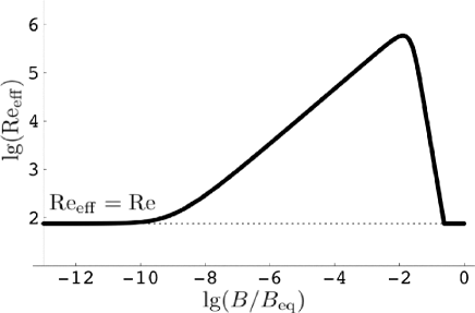
Figure 1: $\text{Re}_{\text{eff}}(B)$: solution of Eq. (11) calculated numerically for the cool-core parameters of Table 1.

Here we would like to leapfrog the rather forbidding task of constructing a quasilinear theory based on the hot plasma dispersion relation with $k\rho_{i}\sim 1$ and instead simply assume that the istabilities saturate with ${\langle\delta B^{2}\rangle/B^{2}}\sim\bigl{(}|\Delta|-{2/\beta}\bigr{)}^{\alpha_{1}}$, where $\Delta=(p_{\perp}-p_{\parallel})/p_{\perp}$, $\beta=2p_{\perp}/B^{2}$, and $\alpha_{1}$ is some positive power. We further assume that the effect of the saturated instabilities is to scatter particles at the rate $\nu_{\text{scatter}}\sim\gamma_{\text{max}}\langle\delta B^{2}\rangle/B^{2}$, where $\gamma_{\text{max}}\sim\bigl{(}|\Delta|-{2/\beta}\bigr{)}^{\alpha_{2}}\Omega_{i}$ is the maximum growth rate of the instabilities ($\alpha_{2}=1$ for the mirror and $\alpha_{2}=1/2$ for the firehose [Eq. (7)]). We may then construct the effective collision rate

$$\nu_{\text{eff}}\sim\nu_{ii}+\nu_{\text{scatter}}\sim\nu_{ii}+\left(|\Delta|-{2\over\beta}\right)^{\alpha}\Omega_{i},$$ (8)

where $\alpha=\alpha_{1}+\alpha_{2}>0$. This changes the characteristics of the turbulence: the effective mean free path of the particles is $\lambda_{\text{mfp,eff}}\sim v_{\text{th},i}/\nu_{\text{eff}}$, the effective (parallel) viscosity of the ICM is $\mu_{\parallel,\text{eff}}\sim v_{\text{th},i}\lambda_{\text{mfp,eff}}$ and, therefore, the effective Reynolds number is

$$\text{Re}_{\text{eff}}\sim{UL\over\mu_{\parallel,\text{eff}}}\sim{UL\over v_{\text{th},i}^{2}}\,\nu_{\text{eff}}.$$ (9)

On the other hand, using Eq. (4) with effective viscosity $\mu_{\parallel,\text{eff}}$ and $|\bm{\nabla}{\bf u}|\sim(U/L)\text{Re}_{\text{eff}}^{1/2}$, we get

$$|\Delta|\sim\left({U\over v_{\text{th},i}}\right)^{2}\text{Re}_{\text{eff}}^{-1/2}.$$ (10)

From Eqs. (8–10), we assemble a (model) equation for the effective Reynolds number:

$$\!\!\text{Re}_{\text{eff}}=\text{Re}+{L\over\rho_{i,\text{eq}}}\left({U\over v_{\text{th},i}}\right)^{\!\!2\alpha+1}\!\!\!\left({1\over\sqrt{\text{Re}_{\text{eff}}}}-{2B^{2}\over B_{\text{eq}}^{2}}\right)^{\alpha}\!\!\!{B\over B_{\text{eq}}},\$$ (11)

where Re is the original Reynolds number based on collisions and $\rho_{i,\text{eq}}$ is the ion gyroradius for $B=B_{\text{eq}}$. The assumption that $\text{Re}_{\text{eff}}$ adjusts to the value of $B$ instantaneously is justified by the fact that the instability growth rates are much faster than all other relevant time scales.

Equation (11) models qualitatively the assumed outcome of an as yet inexistent proper theory of the viscosity of magnetized ICM. Its solution is plotted in Fig. 1. We shall use this model shortly in our discussion of the fluctuation dynamo in clusters.

V Fluctuation dynamo

In Sec. III, we reviewed the observational evidence that testified to the presence of a dynamically significant randomly tangled magnetic field in clusters. What is the origin of this field? There are numerous physical reasons to expect that a certain amount of seed magnetic energy predates structure formation and was, therefore, already present at the birth of clusters.Grasso and Rubinstein (2001); Gnedin et al. (2000) Typical values given for the strength of such field are in the range of $B_{\text{seed}}\sim 10^{-21}-10^{-17}$, although this may be an underestimate.Banerjee and Jedamzik (2003) It then falls to the random motions of the cluster plasma to amplify the field to its observed magnitude of a few $\mu$G. This, indeed, they should be able to do by means of the fluctuation (or small-scale) dynamo mechanism: the random stretching of the field. It is a fundamental property of a succession of random (in time) linear shears that it leads on the average to exponential growth of the energy of the magnetic field frozen into the medium.Batchelor (1950); Zeldovich et al. (1984, 1990) The rate of growth is roughly equal to the rate of strain (shear, or stretching rate) of the random flow. While the mathematical theory of this process can be nontrivial,Arnold and Khesin (1999) the physics of it is basically illustrated by Fig. 2.

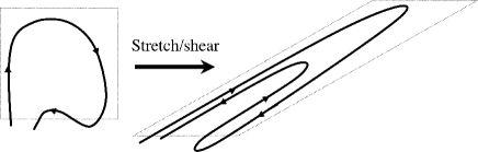
Figure 2: The mechanism of the fluctuation dynamo.

In Kolmogorov turbulence, the rate of strain is dominated by the viscous scale, so $|\bm{\nabla}{\bf u}|\sim t_{\text{visc}}^{-1}\sim(U/L)\text{Re}^{1/2}$. In fact, what is relevant for the growth of the magnetic field is not the full rate-of-strain tensor but its “parallel” component, ${\bf\hat{b}}{\bf\hat{b}}:\bm{\nabla}{\bf u}$. Since this is exactly the type of motion damped by Braginskii viscosity [see Eqs. (4–5)], we can, for the purposes of the fluctuation dynamo, ignore any subviscous-scale velocity fluctuations. Thus, the magnetic field should grow according to

$${1\over B}{dB\over dt}={\bf\hat{b}}{\bf\hat{b}}:\bm{\nabla}{\bf u}\sim{U\over L}\,\text{Re}^{1/2}.$$ (12)

In order to be useful, this amplification has to be done over a time that is shorter than the typical age of the clusters, i.e., a few Gyr. As $L/U\sim 1$ Gyr and as the Reynolds number based on collisional ICM viscosity is quite low, it has been a concern of many authors that the cluster life time might not be (or, possibly, is only just) sufficient to bring the field to its current strengthJaffe (1980); Roland (1981); Ruzmaikin et al. (1989); Young (1992); Goldshmidt and Rephaeli (1993); Sánchez-Salcedo et al. (1998); Subramanian et al. (2006) (this obviously depends on the magnitude of the seed field). Similar issues arise in simulations of the growth of magnetic fields in clusters.Roettinger et al. (1999); Dolag et al. (1999, 2002, 2005); Brüggen et al. (2005) However, if Eq. (11) is a good model of the ICM viscosity, the value of the Reynolds number based on the collisional viscosity has to be amended when the ICM is magnetized: since the prefactor $L/\rho_{i,\text{eq}}$ in the second, magnetic-field dependent term in Eq. (11) is extremely large (see Table 1), this term will dominate already for very small values of the magnetic field strength, namely, for $B>B_{1}$, where

$$B_{1}=B_{\text{eq}}\,{\rho_{i,\text{eq}}\over L}\biggl{(}{v_{\text{th},i}\over U}\biggr{)}^{1+2\alpha}\text{Re}^{1+\alpha/2}.$$ (13)

$B_{1}$ is typically so small (Table 1) that the seed field in clusters may already exceed this value. Thus, the effective Reynolds number of the ICM will be much larger than the one based on collisions. Substituting $\text{Re}_{\text{eff}}$ instead of Re into Eq. (12), we see that, since $\text{Re}_{\text{eff}}\propto B^{2/(2+\alpha)}$ in the weak-field regime, the dynamo is self-accelerating and the field will increase not exponentially but explosively:

$$B(t)\sim{B(0)\over\left(1-t/t_{c}\right)^{2+\alpha}},$$ (14)

where $B(0)\sim$ the greater of $B_{\text{seed}}$ and $B_{1}$ and $t_{c}=(2+\alpha)(L/U)\text{Re}^{-1/2}\left[B_{1}/B(0)\right]^{1/(2+\alpha)}$ is at most (for $B_{\text{seed}}<B_{1}$) the viscous turnover time $t_{\text{visc}}$ associated with the collisional Re. The explosive stage continues until the amplified field starts suppressing the instabilities, i.e., when $\beta$ drops to values comparable to $(v_{\text{th},i}/U)^{2}\text{Re}_{\text{eff}}^{1/2}$. This happens at $B\sim B_{2}$, where

$$B_{2}=B_{\text{eq}}\left[\biggl{(}{v_{\text{th},i}\over U}\biggr{)}^{1+2\alpha}{\rho_{i,\text{eq}}\over L}\right]^{1/(5+2\alpha)}.$$ (15)

Thus, we have a mechanism that amplifies the field by many orders of magnitude from any strength above $B_{1}$ to $B_{2}$ in finite, cosmologically short, time $\sim t_{c}$. The value of $B_{2}$ turns out to be only just over an order of magnitude below $B_{\text{eq}}$ (see Table 1).

Further growth of the field is algebraically slow ($B\sim t^{1/2}$), but it does not have to go on for a very long time because $B_{2}$ is already quite close to the observed field strength. To be precise, there are two algebraic regimes. During the first, $\text{Re}_{\text{eff}}$ is still controlled by the second term in Eq. (11) as $B$ hovers just below $B_{\text{eq}}\text{Re}_{\text{eff}}^{-1/4}$ while $B$ is increasing and $\text{Re}_{\text{eff}}$ is decreasing. Eventually, $B\sim B_{\text{visc}}=B_{\text{eq}}\text{Re}^{-1/4}$ and $\text{Re}_{\text{eff}}$ is returned back to Re (plasma instabilities are suppressed). As this is also the field strength at which the field has energy comparable to the energy of the viscous-scale motions, any further growth of the field is a nonlinear process, in which the back reaction of the field on the flow has to be taken into account. This can be done by assuming that, as the field grows, it can no longer be stretched by motions whose energy it exceeds and that, therefore, at any given time, the dominant stretching is exerted by motions whose energy is equal to that of the field. Denoting their velocity and scale by $u_{l}$ and $l$ and using $u_{l}^{2}\sim B^{2}$, we haveSchekochihin et al. (2002a); Schekochihin et al. (2004)

$${d\over dt}B^{2}\sim{u_{l}\over l}\,B^{2}\sim{u_{l}^{3}\over l}\sim\epsilon=\text{const},$$ (16)

where $\epsilon$ is the energy flux through scale $l$, which, by Kolmogorov’s assumption, is independent of $l$. Thus, $B\sim(\epsilon t)^{1/2}$, the second algebraic regime. Obviously, this can only go on until $l\sim L$, $B\sim B_{\text{eq}}$, and no further amplification is possible.

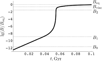
Figure 3: Evolution of the magnetic-field strength for the cool-core parameters of Table 1.

The time evolution of the field is illustrated in Fig. 3, where we plot the result of a numerical integration of Eq. (12) with Re replaced by $\text{Re}_{\text{eff}}$. To implement the idea of the nonlinear suppression of stretching by motions whose energy is smaller than $B^{2}$, we have amended the definition of $\text{Re}_{\text{eff}}$ in the following simple waySchekochihin et al. (2002a)

$$\text{Re}_{\text{eff}}^{\rm(nonlin)}={\text{Re}_{\text{eff}}\over 1-A}\left[{1\over(1+\text{Re}_{\text{eff}}^{1/2}B^{2}/B_{\text{eq}}^{2})^{2}}-A\right],$$ (17)

where $A=1/\bigl{(}1+\text{Re}_{\text{eff}}^{1/2}\bigr{)}^{2}$, so that $\text{Re}_{\text{eff}}^{\rm(nonlin)}=\text{Re}_{\text{eff}}$ when $B\to 0$ and $\text{Re}_{\text{eff}}^{\rm(nonlin)}\to 0$ when $B\to B_{\text{eq}}$. $\text{Re}_{\text{eff}}$ is determined for each value of $B$ by Eq. (11).

VI Magnetized plasma turbulence

Thus, the clusters should have no trouble developing magnetic fields of observed strength over just a fraction of their life time. This, however, is only one part of the problem. The other, much more difficult, part is to determine the spatial structure of the field. TheoryOtt (1998); Schekochihin et al. (2002b) and numerical simulationsSchekochihin et al. (2004); Brandenburg and Subramanian (2005) of the fluctuation dynamo in a conventional MHD formulation with fixed isotropic viscosity and much smaller resistivity ($\text{Rm}\gg\text{Re}$) produce magnetic fields arranged in folded flux sheets whose parallel (locally to themselves) scale is similar to the scale of the velocity that does the stretching, while the field reversal scale in the direction perpendicular to itself is the resistive scale. Fig. 2 illustrates why such a folded structure must be a generic outcome of random stretching. Less obviously, it turns outSchekochihin et al. (2004) that the folded structure is a feature not only of the kinematic growth stage of the dynamo but also of its saturated state (Fig. 4). In the latter case, the fold length is, thus, $l_{\parallel}\sim L$, while the reversal scale is $l_{\perp}\sim l_{\text{res}}\sim L\text{Rm}^{-1/2}$. The magnetic-energy spectra of such fields appear to peak around $k\sim 1/l_{\perp}$.

   

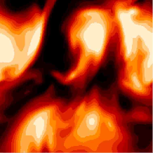
Figure 4: Cross sections of $|{\bf u}|$ (left) and $|{\bf B}|$ (right) in the saturated state of a simulation with $\text{Re}\simeq 100$, $\text{Rm}=1000$ (run B of Ref. Schekochihin et al., 2004).

This prediction is clearly not in agreement with what seems to be the observationally supported picture of the magnetic fields in clusters. While the typical scale $l_{B}$ of the cluster fields is significantly smaller than the outer scale $L$ of the turbulent velocities, it is certainly not the resistive scale — at least not the one based on the standard Spitzer resistivity. What then determines the reversal scale in clusters? While the definite solution of this puzzle remains elusive, we offer the following qualitative argument that at least constrains the answer.

Examining again Fig. 2, it should be obvious that if the folded magnetic field is to reverse its direction, it must turn a corner somewhere and that in that corner, the field should be weaker than in the straight segments of the fold. Furthermore, as there are antiparallel fields in the straight segments themselves, there must be layers of weak field between them (assuming that folds are flux sheets: i.e., that the antiparallel fields in Fig. 2 are, indeed, approximately aligned). These are, in fact, also of the “corner” type: this becomes clear if the fold depicted in Fig. 2 is thought of as a fragment of a larger nested folded structure formed by repeated stretching/shearing and bending. This view of the dynamo-generated fields as either strong and straight or weak and curved is confirmed in numerical simulations, which find an almost perfect anticorrelation between the field’s strength and its curvature.Schekochihin et al. (2004) While the exact quantitative relation between the field strength and its scale may be a nontrivial issue, here we shall continue in the spirit of intuitive reasoning and argue that by flux conservation, $B_{\text{straight}}/B_{\text{corner}}\sim l_{\parallel}/l_{\perp}$ (this again relies on assuming that folds are flux sheets). Thus, the larger is the aspect ratio $l_{\parallel}/l_{\perp}$, the larger is the contrast between the strong field in the straight segments of the folds and the weak field in the corners. We assume that the rms value of the field is determined by the straight segments because these are the fields that are stretched by turbulence. It is their growth that we studied in Sec. V. In the saturated state, we expect $B_{\text{straight}}\sim B_{\text{eq}}$. For such a strong field, the plasma instabilities are suppressed. It is intuitively clear that they must be suppressed in the regions of the weak field as well, i.e., the field there cannot be weaker than $B_{2}$ [Eq. (15)]. Indeed, as we saw in Sec. V, the explosive dynamo mechanism brings any field up to this value nearly instantaneously (for $B>B_{2}$, the growth is much slower). We may conjecture that the maximum aspect ratio of the folds is set by the maximum contrast in the field strength $l_{\parallel}/l_{\perp}\sim B_{\text{eq}}/B_{2}$. Substituting the numbers, we find (Table 1) that this prediction gives the field reversal scale no smaller than a few per cent of the outer scale $L$ (taking $l_{\parallel}\sim L$). This is in passable agreement with the observational evidence, which is the best one can expect, given the highly imprecise nature of our argument, of most observational inferences, and of the definitions of such quantities as $l_{B}$, $l_{\perp}$, $l_{\parallel}$ and $L$. For comparison of our model with observational data for a number of individual clusters, see Ref. Enßlin and Vogt, 2006.

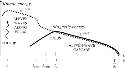
Figure 5: A schematic illustration of the structure of cluster turbulence proposed in Sec. VI.

It is fair to acknowledge that the above argument, while providing a useful constraint, falls short of a satisfactory explanation of the field structure. One might argue that if, in the course of the turbulent stretching/shearing of the field, a region of field strength below $B_{2}$ appears (as explained above, in the corner of a fold), $\text{Re}_{\text{eff}}$ there becomes very large and a localized spot of high-Reynolds-number turbulence is formed. This should have two principal effects. The first is akin to that of a locally enhanced turbulent resistivity, so the field that violates our constraint is continuously destroyed. The second is a burst of explosive fluctuation dynamo in the spot, which produces more folded field with $B>B_{2}$ and thus shuts itself down. These folds are then further stretched, sheared, etc., again subject to the constraint that they are destroyed and replaced by new ones wherever a spot of weak field appears. We do not currently have a more detailed mechanistic scenario of how exactly the folded structure with $l_{\parallel}/l_{\perp}\sim B_{\text{eq}}/B_{2}$ is established. It may be feasible to test these ideas numerically by solving MHD equations with viscosity locally determined by the magnetic-field strength according to Eq. (11).

Let us assume that cluster fields do indeed have a folded structure with a direction reversal scale $l_{\perp}\sim(0.01...0.1)L$, possibly determined by the argument given above. The magnetic-energy spectrum then peaks at $k\sim 1/l_{\perp}$. What is the structure of the turbulence above and below this scale? At scales $l\ll l_{\perp}$, the magnetic field reversing at the scale $l_{\perp}$ will appear uniform and, in accordance with the old idea of KraichnanKraichnan (1965) could support a cascade of Alfvén waves. This cascade can rigorously be shown to be described by the equations of Reduced MHD at collisionless scales all the way down to the ion gyroscale.Schekochihin et al. (2006) The currently accepted theory of such a cascade, primarily associated with the names of Goldreich and Sridhar,Goldreich and Sridhar (1995) is based on the conjecture that at each scale, the Alfvén frequency is equal to the turbulent decorrelation rate. The result is a $k^{-5/3}$ spectrum of Alfvénic fluctuations — this possibly explains what appears to be a $k^{-5/3}$ tail in the observed spectrum of magnetic energy for the Hydra A core.Vogt and Enßlin (2005) We cannot embark on a detailed discussion of the theory of the Alfvén-wave cascade here, so the reader is referred to Ref. Schekochihin and Cowley, 2006 for a review and to Ref. Schekochihin et al., 2006 for the theoretical basis of extending this theory to collisionless scales.

Above the reversal scale, $l\gg l_{\perp}$, the cluster turbulence should resemble the saturated state of isotropic MHD turbulence: a magnetic-energy spectrum with a positive spectral index corresponding to folded fields and a kinetic-energy spectrum populated in the inertial range by a peculiar type of Alfvén waves that propagate along the folds (i.e., simultaneously perturbing the antiparallel magnetic field lines).Schekochihin et al. (2002a); Schekochihin et al. (2004) This type of turbulence is also reviewed in Ref. Schekochihin and Cowley, 2006. It is probably of limited relevance for clusters because the Reynolds number in the ICM is not large enough to allow a well-developed inertial range.

Fig. 5 summarizes the — admittedly, rather speculative — picture of cluster turbulence proposed above. We offer this sketch in lieu of conclusions. While we believe that the set of physical arguments that has led to it is not without merit, it is clear that much analytical, numerical and observational work is needed before a conclusion can truly be reached in the study of turbulence, magnetic fields and plasma physics in clusters of galaxies.