Element abundances of unevolved stars in the open cluster M 67

Abstract

Context. The star-to-star scatter in lithium abundances observed among otherwise similar stars in the solar-age open cluster M 67 is one of the most puzzling results in the context of the so called “lithium problem”. Among other explanations, the hypothesis has been proposed that the dispersion in Li is due to star-to-star differences in Fe or other element abundances which are predicted to affect Li depletion.

Aims. The primary goal of this study is the determination of the metallicity ([Fe/H]), $\alpha$- and Fe-peak abundances in a sample of Li-poor and Li-rich stars belonging to M 67, in order to test this hypothesis. By comparison with previous studies, the present investigation also allows us to check for intrinsic differences in the abundances of evolved and unevolved cluster stars and to draw more secure conclusions on the abundance pattern of this cluster.

Methods. We have carried out an analysis of high resolution UVES/VLT spectra of eight unevolved and two slightly evolved cluster members using MOOG and measured equivalent widths. For all the stars we have determined [Fe/H] and element abundances for O, Na, Mg, Al, Si, Ca, Ti, Cr and Ni.

Results. We find an average metallicity [Fe/H] $=0.03\pm 0.01$, in very good agreement with previous determinations. All the [X/Fe] abundance ratios are very close to solar. The star-to-star scatter in [Fe/H] and [X/Fe] ratios for all elements, including oxygen, is lower than 0.05 dex, implying that the large dispersion in lithium among cluster stars is not due to differences in these element abundances. We also find that, when using a homogeneous scale, the abundance pattern of unevolved stars in our sample is very similar to that of evolved stars, suggesting that, at least in this cluster, RGB and clump stars have not undergone any chemical processing. Finally, our results show that M 67 has a chemical composition that is representative of the solar neighborhood.

1 Introduction

“Classical” or “standard” models of stellar evolution include convection only as internal mixing process and neglect more complex physical processes like diffusion, magnetic fields, rotation; these models predict that solar-type stars should not deplete lithium (Li) while on the main sequence (MS), since the base of the convective zone does not reach the layers in the stellar interior where the temperature is high enough for Li reactions. Furthermore, according to standard models, stars with the same age, mass, and chemical composition should undergo the same amount of Li depletion. In sharp contrast with these predictions, not only is now well established on observational grounds that solar-type stars, including the Sun, do deplete a significant amount of Li during the MS phases, but Li depletion can be different for similar stars (e.g., Randich r_cast (2006) and references therein). The factor of about 10 star-to-star scatter in Li abundances observed among otherwise identical F- and G-type members of the 4.5 Gyr old cluster M 67 indeed represents one of the most puzzling results in the context of the so-called “Lithium problem” (Spite et al. spi87 (1987); Garcia López et al. gar88 (1988); Pasquini et al. pas97 (1997); Jones et al. jon99 (1999)).

A large dispersion in Li abundances is present among old field stars (e.g., Pallavicini et al. pal87 (1987); Pasquini et al. pas94 (1994)). On the other hand, whereas no dispersion is seen in the 600 Myr old Hyades, in the three 2 Gyr old clusters IC 4651, NGC 3680 and NGC 752 (Randich et al. r00 (2000); Sestito et al. ses_752 (2004)), nor in 6 Gyr old NGC 188 (Randich et al n188 (2003)), preliminary results of Li measurements among large samples of stars in the 2 Gyr, metal rich NGC 6253 and in the very old Collinder 261 suggest that they could be characterized by some amount of scatter (Pallavicini et al. pall_cast (2006); Randich r_cast (2006)). In other words, the appearance of a dispersion seems to depend more on the characteristics of the cluster than on age.

It has been shown that non membership and/or binarity are not the reasons for the scatter in M 67 (Pasquini et al. pas97 (1997)); also, the effects of chromospheric activity on the formation of the Li i line, which are proposed as a possible explanation for the dispersion in young clusters (Jeffries jef_06 (2006) and references therein), are unlikely to play a role, given that at the old age of M 67 the level of chromospheric activity should be low enough not to affect the Li i line. Hence, the scatter is most likely intrinsic and, under the very reasonable assumption that cluster stars were all born with the same Li content, it must reflect different amounts of Li depletion.

Different possibilities were proposed to explain the existence of the spread (Randich r_cast (2006)); among them, it has been suggested that M 67 members do not have an identical chemical composition and that the scatter in Li may reflect a scatter in iron content or, more in general, in heavy element composition (Garcia López et al. gar88 (1988); Piau et al. piau03 (2003)).

As well known, chemical composition affects stellar opacities and thus internal structure, mixing processes (both standard and non standard ones) and, in principle, Li depletion. The effect of variations of the chemical composition on pre-main sequence Li depletion has been theoretically investigated in different studies (e.g, Swenson et al. sf_92 (1992); Piau & Turck-Chieze ptc (2002); Sestito et al. ses_06 (2006)) and all of them agree in that even relatively small changes of the mass fraction of elements critical for the opacity can have significant effects on the amount of Li depletion. Similarly, Piau et al. (piau03 (2003)) have shown that variations in CNO abundances can change the amount of Li depletion during the MS phases and suggested that star-to-star differences in these element abundances or, more in general in $\alpha$ and Fe-peak abundances, could explain the observed scatter in M 67. More quantitatively, they found that a difference of 0.05 dex in [CNO/Fe] would result in a difference in $\log$ n(Li) of $\sim 0.5$ dex (i.e, smaller than the observed spread), implying that larger differences in CNO abundances are needed to explain the whole spread.

Garcia López et al. (gar88 (1988)) did not find any difference in the overall metallicity of Li-poor and Li-rich stars and ruled out that different [Fe/H] values within M 67 could be the reason for the scatter in Li. Here we extend their work to elements other than iron and to a larger sample of stars, to investigate a) whether a large ($>0.05$ dex) star-to-star scatter in heavy elements is present among unevolved cluster members; and, in case such a spread is detected, b) whether it is related to the dispersion in Li.

In a more general context, the determination of the metallicity and chemical composition of open clusters covering a large interval of ages, metallicities, and Galactocentric distances is a critical tool to investigate the formation and evolution of the Galactic disk (Friel friel (2006) and references therein). M 67 is one of the closest and best studied old open clusters; nevertheless, relatively few studies focused on the determination of its chemical composition (Tautvaišienė et al. tau00 (2000) and references therein), and most of them are based on few and/or evolved stars that may have undergone chemical processing. The present work represents the first abundance study of M 67 based on a rather large sample of unevolved (or slightly evolved) cluster members, allowing us to check whether intrinsic differences exist between abundances of unevolved and evolved stars and to draw more secure conclusions on the abundance pattern of this cluster. The paper is structured as follows: in Sect. 2 the sample and the observations are described, while the abundance analysis is presented in Sect. 3. The results, together with a discussion of internal and systematic errors, and a comparison with findings from previous studies are presented in Sect. 4. Finally, a discussion of the results and conclusions are given in Sect. 5.

2 Sample and observations

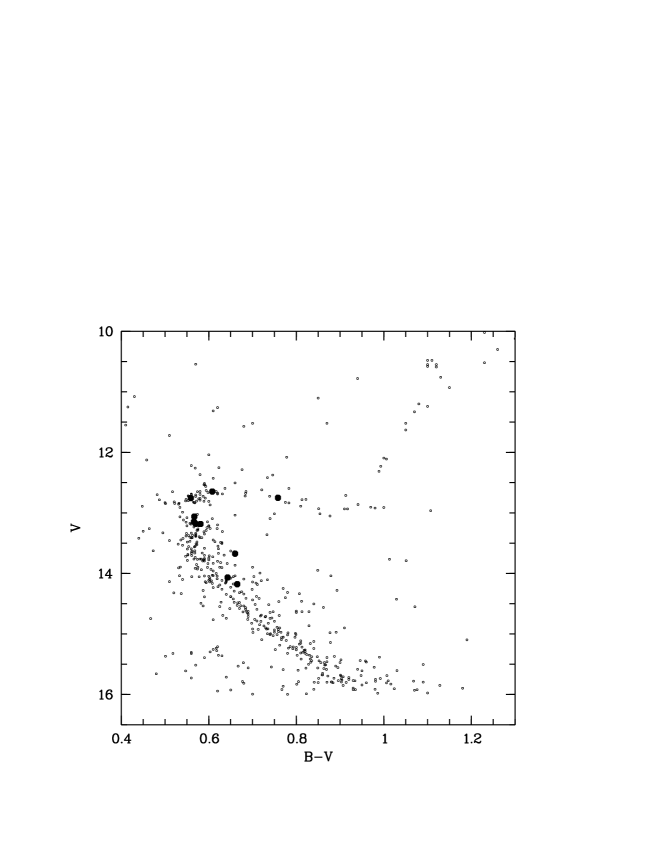
Figure 1: Color-magnitude diagram of M 67. The sample stars are indicated as filled circles. CCD photometry was taken from Montgomery et al. (mont93 (1993)). Only stars brighter than V=16 are plotted in the figure.

Our sample includes 10 single M 67 members that are listed in Table 1, together with V, $B-V$, and ($B-V)_{0}$ colors. The color-magnitude diagram of the cluster with our sample stars evidenced in black is shown in Fig. 1; the diagram indicates that seven of them are still on the MS, one is close to the the turn-off, while the remaining two are already evolved to the subgiant branch.

The observations were obtained using the UVES spectrograph (Dekker et al. dek (2002)) on VLT UT2/Kueyen during three different observing runs; the first one was carried out in Visitor mode in April 2000, while the other two were performed in Service mode in Fall 2001 and Spring 2002, respectively. Details on the observations, whose primary goal was the measurement of beryllium abundances in the sample stars, were already given in Randich et al. (R02 (2002)) and we summarize the main points in the following. UVES was operated in Dichroic Mode using Cross Dispersers #1 and #3 in the Blue and Red arms, respectively. The Red arm, which is of interest here, is equipped with a mosaic of two CCDs composed by a EEV 2048$\times$4102 CCD and a MIT-LL $2048\times 4102$ CCD; the spectral coverage ranges from approximately 4780 to 6810 Å. The 15$\mu m$ pixels together with a 1 arcsec wide slit (projecting onto 4 pixels) and CCD binning $1\times 1$, yielded a resolving power R$\sim 45,000$. Exposure times were set based on the requirement of a good S/N ratio in the near-UV spectral regions where the Be ii lines are located and range between 1.3 and 3 hrs per star. Data reduction was carried out using the UVES pipeline and following the usual steps. Typical $S/N$ ratios per resolution element measured on the extracted 1-D spectra range between 90 and 180.

Table 1: Sample stars, photometry, stellar parameters and derived metallicities together with rms scatter. Numbering is from Sanders (sand (1977)). V magnitudes and $B-V$ colors were taken from Montgomery et al. (mont93 (1993)). ($B-V)_{0}$ colors were instead retrieved from Jones et al. (jon99 (1999)) who had derived them based on original $B-V$ and $V-I$ colors of Montgomery et al. and assuming a reddening E($B-V)=0.05$. For stars S1034 and S1239, not included in the sample of Jones et al. (jon99 (1999)), we obtained ($B-V)_{0}$ colors in the same way. One Hyades member is also included (see text).

S	V	$B-V$	($B-V)_{0}$	Teff	$\xi$	$\log$ g	[Fe/H]i	rms
				(K)	(km/s)
969	14.18	0.665	0.622	5800	1.10	4.4	0.01	0.04
988	13.18	0.570	0.534	6153	1.45	4.1	0.03	0.04
994	13.18	0.581	0.535	6151	1.45	4.1	0.0	0.04
995	12.76	0.559	0.521	6210	1.50	3.9	0.05	0.03
998	13.06	0.567	0.518	6223	1.50	4.0	0.07	0.05
1034	12.65	0.608	0.567	6019	1.50	4.0	0.01	0.05
1239	12.75	0.758	0.692	5541	1.25	3.8	0.02	0.03
1252	14.07	0.643	0.588	5938	1.15	4.4	0.05	0.03
1256	13.67	0.660	0.595	5907	1.10	4.5	0.06	0.03
2205	13.14	0.566	0.534	6156	1.45	4.1	0.00	0.05
vB 187	9.01	0.76	0.75	5339	0.9	4.5	0.13	0.05

3 Abundance analysis

Abundance analysis was carried out by means of measured equivalent widths ($EW$s) and using Version 2000 of MOOG (Sneden sne_moog (1973)) with a grid of 1-D model atmospheres from Kurucz (kur93 (1993)). We recall that MOOG performs a standard-LTE analysis.

3.1 Line list and equivalent widths

Spectral lines to be used for the analysis of Fe i, Fe ii and, other elements (Na, Mg, Al, Si, Ca, Ti, Cr, Ni) were selected from different sources in the literature and subsequently checked for suitability (in particular for blends) on the solar spectrum obtained with UVES at the same resolution as our sample stars. We finally retained in the list 55 Fe i and 11 Fe ii lines, and a total of approximately 70 lines for all the other elements.

The task eq in SPECTRE was used to interactively measure the $EW$s of the spectral lines by gaussian fitting. Although the spectra had been previously normalized, local continuum was inspected and, if needed, adjusted at each $EW$ measurement.

3.2 Atomic parameters and solar analysis

The majority of $\log gf$ values for both Fe and other element lines were taken from the Vienna Atomic Line Data-base (VALD: Piskunov et al. pis95 (1995); Kupka et al kup99 (1999): Ryabchikova et al. rya99 (1999) — http://www.astro.uu.se/htbin/vald). For a few lines for which $\log gf$ from VALD were not available or gave very discrepant abundances for the Sun, $\log gf$ were either taken from other sources in the literature or, in a few cases, adjusted through an inverse solar analysis. Note that $\log gf$ values for all Fe i lines were taken from VALD. In Table 2 we show all the lines included in our list together with their $\log gf$ values, the source for these values, and the $EW$s measured in the solar spectrum. Radiative and Stark broadening are treated in a standard way in MOOG; as for collisional broadening, we used the Unsöld approximation (uns (1955)) for all the lines. As discussed by Paulson et al. (paul03 (2003)) this choice should not greatly affect the differential analysis with respect to the Sun. We also mention that very strong lines that are most affected by the treatment of damping have been excluded from our analysis.

The analysis of the solar spectrum was performed assuming the following solar parameters: T${}_{\rm eff\;\odot}=5770$ K, $\log g_{\odot}=4.44$ and $\xi_{\odot}=1.1$ km/s. We mention that $\log$ n(Fe i) vs. $EW$ did not show any trend, implying that the assumed microturbulence is correct. On the contrary we found a small, but statistically significant (slope equal to 0.009, correlation coefficient 0.326) trend of Fe i abundances vs. excitation potential (EP). Such a trend would disappear by assuming a 70 K higher solar effective temperature (T_eff${}_{\odot}=5840$ K), which would result in larger and smaller abundances for Fe i and Fe ii, respectively ($\log$ n(Fe i)=7.58 and $\log$ n(Fe ii)=7.49).

Output solar abundances are listed in Table 3 together with those from Anders & Grevesse (ag89 (1989)) that are used as input in MOOG. Note that, although solar abundances from Anders & Grevesse (ag89 (1989)) have been superseded by the study of Grevesse & Sauval (grsa_98 (1998)), the two studies yield the same abundances or very little differences for the elements analyzed in this study. Table 3 shows a good agreement between the abundances determined by us and the values of Anders & Grevesse (ag89 (1989)), the most discrepant element being Na with $\Delta\log$(Na)=0.05 dex. We also find a very good agreement between $\log$ n(Fe) from Fe i and Fe ii.

Table 3: Solar abundances from Anders & Grevesse (ag89 (1989)) and those determined through our analysis. Note that $\log gf$ values for Al were derived by an inverse solar analysis.

Element	$\log$ n(X)AG89	$\log$ n(X)our
O i	8.87	8.66$\pm 0.04$
Na i	6.33	6.28$\pm 0.03$
Mg i	7.58	7.57$\pm 0.01$
Al i	6.47	6.47$\pm 0.03$
Si i	7.55	7.56$\pm 0.03$
Ca i	6.36	6.35$\pm 0.02$
Ti i	4.99	4.97$\pm 0.02$
Cr i	5.67	5.65$\pm 0.02$
Fe i	7.52	7.52$\pm 0.03$
Fe ii	7.52	7.51 $\pm 0.04$
Ni i	6.25	6.25 $\pm 0.03$

3.3 Oxygen

We do not discuss here all the intricacies related to oxygen abundance determinations in stars, and we refer to Bensby et al. (bensby04 (2004)) and Schuler et al. (schuler (2005)) for recent discussions. The forbidden lines at 6300.30 Å and 6363.78 Å are not significantly sensitive to NLTE effects nor to stellar effective temperature; therefore, as widely acknowledged, these lines are the most reliable ones for deriving O abundances. Our O determinations are based on the [O i] forbidden line at 6300.3 Å. Although this line is located in a spectral region that is severely affected by the presence of telluric lines, the radial velocity of M 67 is such that they do not affect the [O i] line in our spectra.

As first pointed out by Lambert (lambert (1978)), the 6300.3 Å  line is blended with a Ni i feature whose contribution must be taken properly into account for an accurate determination of O abundance. Hence, we determined O both for the Sun and our sample stars using the driver blend in MOOG, that allows accounting for the blending Ni i 6300.34 feature when force fitting the abundance of the O to the measured $EW$s of the 6300.3 Å feature. As done for the other lines, $EW$s of the 6300.3 Å feature were measured by gaussian fitting using SPECTRE. The solar [O i] $EW$ measured in the UVES spectrum is 5.5 $\pm 0.3$ mÅ, in good agreement with previous estimates (see Schuler et al schuler (2005)); $EW$s for the sample stars are listed in the second column of Table 5.

For our analysis we employed the [O i] $gf$-value determined by Allende Prieto et al. (ap01 (2001)), $\log\leavevmode\nobreak\ gf=-9.717$, while for the Ni i 6300.34 Å blend, following Johansson et al. (joha03 (2003)), we used $\log\leavevmode\nobreak\ gf=-2.11$. Note that, as discussed by Schuler et al., we would have obtained virtually the same O abundances by considering the two separate components of the Ni i blend. Assuming a solar Ni abundance $\log$ n(Ni)=6.25 (see Table 3), we obtained for the Sun $\log$ n(O)=8.66 $\pm 0.04$, much below the classical value of Anders & Grevesse (ag89 (1989)), but in good agreement with recent determinations, including those obtained using 3-D analysis (see again the discussion in Schuler et al.).

3.4 Stellar parameters

Initial stellar parameters for the sample stars were estimated from photometry (see Table 1). Effective temperatures were retrieved from Jones et al. (jon99 (1999)), who, in turn, had derived them using the calibration of Soderblom et al. (sod93 (1993)), i.e, T_eff$=1808\times(\rm B-\rm V)_{0}^{2}-6103\times(B-V)_{0}+8899$. Microturbulence velocities were estimated as: $\xi=3.2\times 10^{-4}(\rm T_{\rm eff}-6390)-1.3(logg-4.16)+1.7$ (Nissen nis81 (1981)), while surface gravities were derived using the relationship: $\log g=4.44+\log\rm M/\rm M_{\odot}+4\log\rm T_{\rm eff}/\rm T_{\rm eff}\;{\odot}+0.4(\rm M_{\rm bol}-\rm M_{\rm bol}\;{\odot}$). Absolute bolometric magnitudes were determined from V magnitudes, adopting a distance modulus (m–M)₀=9.6 (Pace et al. pace_04 (2004): Sandquist san04 (2004)) and assuming bolometric corrections from Johnson (john_66 (1966)). Finally, stellar masses were derived following Balachandran (bala95 (1995)).

In order to determine spectroscopic temperatures one would need to change the initial T_eff values until no $\log$ n(Fe)i vs. EP trend is seen. However, we decided not to change initial T_eff derived from photometry, since a trend is present for the solar spectrum and for all the sample stars we found similar slopes (in magnitude and sign). To further test the correctness of our approach, for each star we plotted $\Delta$$\log$ n(Fe)$=$ $\log$ n(Fe)${}_{\odot}-$$\log$ n(Fe)_star as a function of EP and checked that no significant residual trends were present. Spectroscopic microturbulence values for each star were instead obtained by changing the input microturbulence until no $\log$ n(Fe) vs. $EW$ trends were seen. Finally, $\log$ g values were varied only when necessary, in order to have a difference between iron abundances derived from Fe i and Fe ii lines not greater than 0.05 dex, i.e., consistent, within errors, with the ionization equilibrium. It turned out that we needed to change the initial values of gravity for two stars only, S1239 and S1256. Assumed parameters for the sample stars are listed in Cols. 5–7 in Table 1.

4 Results

4.1 Abundances

Log n(X) values for each line were determined based on measured $EW$s and stellar parameters listed in Table 1. Final abundances for each star and each element were determined as the mean abundance from the different lines. 1$\sigma$ clipping was performed for iron, but not for the other elements for which a smaller number of lines was available. As to oxygen, [O/H] and [O/Fe] values for the sample stars were obtained from the measured $EW$ of the 6300.3 Å blend (see Table 5) and assuming Ni abundances determined through our analysis. As already mentioned, [Fe/H] and [X/Fe] ratios for each star were determined differentially with respect to solar abundances listed in Table 3.

[Fe/H]i abundances and rms values for the sample stars are listed in Cols. 8 and 9 of Table 1, while in Fig. 2 we show [Fe/H] as a function of effective temperature. The figure clearly shows that no trend of [Fe/H] as a function of T_eff is present.

Table 4: Derived abundance ratios for M 67 stars and one Hyades member. For each star, quoted errors on abundance ratios are the quadratic sum of rms values of [Fe/H] and [X/H]. Average abundance ratios for the Hyades, taken from Friel (friel (2006)), are given in the last line.

S	[Na/Fe]	[Mg/Fe]	[Al/Fe]	[Si/Fe]	[Ca/Fe]	[Ti/Fe]	[Cr/Fe]	[Ni/Fe]
969	$0.00\pm 0.06$	$-0.01\pm 0.05$	$-0.01\pm 0.07$	$-0.01\pm 0.06$	$0.09\pm 0.06$	$0.00\pm 0.07$	$0.00\pm 0.06$	$-0.04\pm 0.07$
988	$0.12\pm 0.04$	$0.03\pm 0.13$	$-0.04\pm 0.06$	$0.10\pm 0.05$	$0.12\pm 0.06$	$0.00\pm 0.06$	$0.09\pm 0.04$	$0.03\pm 0.06$
994	$0.12\pm 0.05$	$0.02\pm 0.09$	$-0.04\pm 0.04$	$0.02\pm 0.07$	$0.07\pm 0.06$	$0.04\pm 0.06$	$0.03\pm 0.05$	$0.04\pm 0.06$
995	$0.04\pm 0.04$	$0.00\pm 0.13$	$-0.06\pm 0.08$	$0.03\pm 0.06$	$0.05\pm 0.05$	$-0.06\pm 0.08$	$-0.04\pm 0.04$	$-0.07\pm 0.04$
998	$0.08\pm 0.06$	$0.00\pm 0.09$	$-0.08\pm 0.07$	$-0.02\pm 0.07$	$0.01\pm 0.07$	$0.00\pm 0.08$	$-0.05\pm 0.05$	$-0.03\pm 0.06$
1034	$0.07\pm 0.06$	$-$0.02$\pm 0.05$	$-0.08\pm 0.04$	$0.03\pm 0.06$	$0.03\pm 0.06$	$0.00\pm 0.07$	$0.00\pm 0.05$	$-0.03\pm 0.07$
1239	$0.03\pm 0.09$	$-$0.01$\pm 0.09$	$0.02\pm 0.06$	$0.05\pm 0.07$	$0.00\pm 0.07$	$-0.05\pm 0.05$	$-0.01\pm 0.05$	$-0.03\pm 0.05$
1252	$-0.04\pm 0.06$	$-0.04\pm 0.03$	$-0.09\pm 0.06$	$0.00\pm 0.05$	$0.02\pm 0.04$	$-0.08\pm 0.06$	$-0.04\pm 0.04$	$-0.05\pm 0.05$
1256	$-0.06\pm 0.04$	$-0.04\pm 0.04$	$-0.11\pm 0.05$	$-0.03\pm 0.05$	$0.04\pm 0.06$	$-0.04\pm 0.05$	$-0.02\pm 0.07$	$-0.04\pm 0.05$
2205	$0.13\pm 0.06$	$0.03\pm 0.07$	$-0.06\pm 0.08$	$0.04\pm 0.08$	$+0.03\pm 0.06$	$-0.06\pm 0.09$	$-0.01\pm 0.05$	$0.03\pm 0.06$
vB187	$+0.00\pm 0.05$	$-0.06\pm 0.02$	$-0.07\pm 0.07$	0.07 $\pm 0.07$	$0.04\pm 0.06$	$-0.09\pm 0.04$	$-0.05\pm 0.02$	$0.03\pm 0.06$
Hyadeslit.	$0.01$	$-0.06$	$-0.05$	$0.04$	$+0.06$	$-0.06$	—	—

Table 5: [O i] 6300 Å line $EW$s, [O/H] and [O/Fe] values for the sample stars and the Hyades member. Quoted errors in [O/H] are due to uncertainties in $EW$s, while errors in [O/Fe] are the quadratic sums of errors in [O/H] and rms values of [Fe/H] (see Table 1). In the last line we provide average [O/H] and [O/Fe] ratios for the Hyades from Schuler et al. (schuler (2005)).

S	$EW$ (6300.3 Å)	[O/H]	[O/Fe]
	(mÅ)
969	5.6 $\pm 0.5$	0.02 $\pm 0.06$	0.01 $\pm 0.07$
988	5.3 $\pm 0.9$	0.00 $\pm 0.10$	$-0.03\pm 0.11$
994	5.0 $\pm 0.9$	$-0.03\pm 0.10$	$-0.03\pm 0.11$
995	6.6 $\pm 0.9$	$+0.08\pm 0.08$	$0.03\pm 0.08$
998	5.7 $\pm 0.5$	$+0.04\pm 0.04$	$-0.03\pm 0.06$
1034	6.5 $\pm 0.5$	$+0.03\pm 0.04$	$+0.02\pm 0.06$
1239	10.2 $\pm 1$	$+0.03\pm 0.06$	$+0.01\pm 0.07$
1252	5.1 $\pm 0.4$	$+0.00\pm 0.05$	$-0.05\pm 0.06$
1256	5.0 $\pm 0.5$	$+0.03\pm 0.05$	$-0.03\pm 0.07$
2205	5.4 $\pm 1$	$+0.01\pm 0.11$	$0.01\pm 0.12$
vB187	5.6 $\pm 0.4$	$-0.19\pm 0.08$	$-0.32\pm 0.09$
HyadesSchuler		0.19	0.10

Using all the stars in our sample, we obtain a mean value [Fe/H]$=0.03\pm 0.01$ (rms$=0.03$, 10 stars), very close to solar. This mean value is listed in the first column of Table 7.

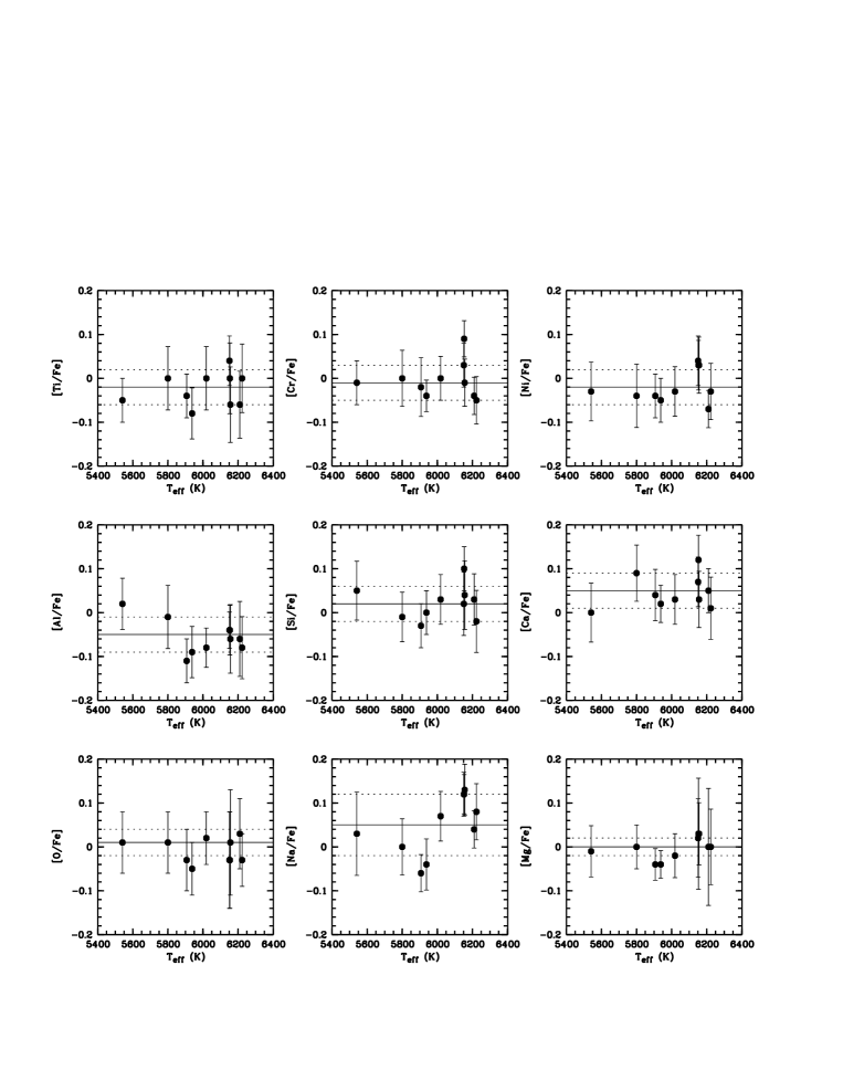
Figure 3: [X/Fe] as a function of effective temperature for the sample stars. Error bars correspond to the quadratic sum of the rms of [Fe/H] (or errors due to uncertainties in measured $EW$s for O, whose abundance has been determined from one line only) and rms of [X/H]. As in Fig. 2, in each panel the solid and dotted lines represent the mean value $\pm 1$ standard deviation.

The [X/Fe] ratios for Na, Mg, Al, Si, Ca, Ti, Cr and Ni are listed in Table 4. Errors on [X/Fe] values in Table 4 correspond to the quadratic sum of rms of [Fe/H] and [X/H] values. Results for O are listed separately in Table 5, where both [O/H] and [O/Fe] values are given; in this case errors in [O/H] correspond to uncertainties in the measured $EW$s of the forbidden line, while errors in [O/Fe] are the quadratic sum of errors in [O/H] and rms of [Fe/H]. Mean abundance ratios for M 67 together with 1$\sigma$ standard deviation are listed in the second column of Table 7, while [X/Fe] ratios for all elements are plotted in Fig. 3 as a function of effective temperature. The figure shows that, as in the case of [Fe/H], no evident trends of [X/Fe] ratios with T_eff are present. A small amount of star-to-star scatter might be present, both in [Fe/H] and [X/Fe] ratios, but for all the elements the scatter is well within measurement uncertainties. A more detailed discussion on the possible presence of a scatter will be provided in Sect. 5.1.

4.2 Errors

Sources of internal errors include uncertainties in atomic and stellar parameters, as well as errors in measurements of $EW$s. The sample spectra are characterized by different S/N ratios and it is not possible to estimate a typical error in $EW$s; however, errors in the derived abundances due to errors in $EW$s are in a good approximation represented by the standard deviation (or rms) around the mean abundance determined from individual lines. The rms in principle includes also errors due to uncertainties in atomic parameters, but the latter should be minimized in our analysis, since it is carried out differentially with respect to the Sun and our stars have parameters (T_eff, $\xi$, $\log$ g) close to the solar ones. As already mentioned, rms values for [Fe/H] are listed in Table 1, while errors in [X/Fe] ratios listed in Table 4 correspond to the quadratic sum of rms for [Fe/H] and rms for [X/H].

Errors in [O/H] include in principle uncertainties in the measurement of the $EW$ of the [O i] 6300.3 Å feature and errors due to uncertainties in Ni abundance, which affect the estimate of the contribution of the Ni I 6300.34 blend to the [O i] feature. We find however that the latter are much smaller than typical errors in [O i] $EW$s. Our spectra are not characterized by an extremely high S/N in the forbidden line region and thus errors in $EW$s are significant. Typical errors are of the order of 0.5-1 mÅ, which reflect into uncertainties in [O/H] between 0.05 and 0.1 dex. On the other hand, uncertainties in Ni abundance are of the order of 0.05 dex at most and correspond to errors in the Ni i $EW$ of the order of 0.15-0.2 mÅ.

Internal errors due to uncertainties in stellar parameters were estimated by varying each parameter separately, while leaving the other two unchanged. We assumed random uncertainties of $\pm 70$ K, $\pm 0.15$ km/s, and $\pm 0.25$ dex in T_eff, $\xi$ and $\log$ g, respectively. We performed different tests and found that for all the stars, T_eff variations larger than 70 K would have introduced significant (i.e, much larger than in the Sun) trends of $\log$ n(Fe i) vs. EP, while variations in $\xi$ larger than 0.15 km/s would have resulted in significant trends of $\log$ n(Fe) vs. $EW$. This applied not only to Fe, but also to the other elements with several lines covering large dynamical ranges in EP and $EW$s. Finally, differences in $log$ g larger than 0.25 dex would have resulted in differences between $\log$ n(Fe i) and $\log$ n(Fe ii) larger than 0.05 dex. In Table 6 we list errors in [Fe/H] and [X/Fe] ratios due to uncertainties in stellar parameters for the coolest (S1239) and one of the warmest (S988) stars in the sample.

Systematic errors are more difficult to evaluate. Errors in the scale of T_eff are likely small, since, as already noted, we did not find major trends of inferred Fe abundances as a function of EP. By using the T_eff vs. $B-V$ calibration of Alonso et al. (al96 (1996)), we would have obtained slightly cooler temperatures, with differences ranging between 40 and 60 K, that would have given a mean metallicity [Fe/H]=$-0.01$ (i.e., 0.04 dex below our estimate) and almost identical [X/Fe] values. More in general, in order to get an estimate of global systematic errors, we analyzed the spectrum of one Hyades member (vB187) observed with the same UVES set-up as our sample stars (complete results on the chemical analysis of other Hyades members will be reported elsewhere). The results for [Fe/H] and [X/Fe] for the Hyades member are listed in Tables 1, 4, and 5; our determination of the metallicity for this star is in perfect agreement with the classical value for the Hyades (Boesgaard & Friel bf90 (1990); Paulson et al. paul03 (2003); Friel friel (2006)); as for the other elements, relatively few abundance determinations have been carried out in the past, in spite of the fact that the Hyades is one of the best studied open clusters. In the last line of Tables 4 and 5 we list the average [X/Fe] ratios for the Hyades taken from the compilation of Friel (friel (2006) —Table 1 in that paper). Our [X/Fe] ratios for most elements are in good agreement with the values from the literature, suggesting that our abundance scale should not be affected by major systematic errors. On the other hand, for vB187 we derive an O abundance (and [O/Fe] ratio) considerably below the average value of Schuler et al. (schuler (2005)). We note however that the discrepancy is most likely due to differences in the $EW$s of the forbidden line, rather than to the analysis. For vB187 we measure an $EW$ of the [O i] 6300.3 Å line of 5 mÅ to be compared with values of 7-8 mÅ found by Schuler et al. for stars with similar temperatures as vB187. Assuming their $EW$s, we would have inferred an [O/H] similar to their values.

Table 6: Random errors due to uncertainties in stellar parameters.

S1239: Teff=5477 K, $\log$ g=3.6, $\xi=1.2$ km/s
$\Delta$	$\Delta$Teff$=\pm 70$	$\Delta\log$g=$\pm 0.25$	$\Delta\xi=\pm 0.15$
	(K)	dex	km/s
[Fe/H]i	0.06/$-0.04$	$-0.01$/0.02	$-0.05$/0.06
[O/Fe]	$-$0.05/0.03	0.12/$-$0.14	$0.05$/$-0.06$
[Na/Fe]	$-$0.01/0.00	$-0.03$/0.01	$0.03$/$-0.03$
[Mg/Fe]	$-$0.01/0.00	$-0.06$/0.05	$0.02$/$-0.03$
[Al/Fe]	$-$0.02/0.00	$0.00$/$-$0.01	$0.04$/$-0.05$
[Si/Fe]	$-$0.05/0.04	0.03/$-0.03$	$0.03$/$-0.04$
[Ca/Fe]	0.0/$-0.02$	$-0.04$/0.01	$-0.01$/0.01
[Ti/Fe]	0.02/$-0.04$	$0.00$/$-$0.01	$0.01$/$-0.02$
[Cr/Fe]	0.03/$-$0.03	$-0.01$/0.0	$-0.02$/0.02
[Ni/Fe]	$-$0.01/0.01	0.02/$-0.03$	$0.01$/$-0.01$
S988: Teff=6151 K, $\log$ g=4.1, $\xi=1.45$ km/s
$\Delta$	$\Delta$Teff$=\pm 70$	$\Delta\log$g=$\pm 0.25$	$\Delta\xi=\pm 0.15$
	(K)	dex	km/s
[Fe/Hi]	0.05/$-0.05$	$-0.02$/0.02	$-0.03$/0.04
[O/Fe]	$-$0.04/0.04	0.13/$-$0.14	$0.03$/$-0.04$
[Na/Fe]	$-$0.02/0.01	$-0.02$/0.01	$0.01$/$-$0.03
[Mg/Fe]	$-$0.01/0.01	$-0.05$/0.05	$0.02$/$-$0.03
[Al/Fe]	$-$0.02/0.02	$0.01$/$-$0.01	$0.02$/$-$0.04
[Si/Fe]	$-$0.02/0.03	0.02/$-0.01$	$0.02$/$-$0.03
[Ca/Fe]	0.00/0.00	$-0.02$/0.02	$-0.01$/0.01
[Ti/Fe]	0.01/$-0.01$	$0.01$/$-$0.01	$0.02$/$-$0.02
[Cr/Fe]	0.01/$-0.02$	$0.00$/$-$0.01	$-0.02$/0.0
[Ni/Fe]	$-$0.01/0.0	$0.01$/$-$0.02	$0.01$/$-$0.02

4.3 NLTE effects and 3-D

As well known, the assumption of LTE may introduce systematic errors and may give origin to spurious abundance trends when analyzing stars covering large intervals of effective temperatures, gravities and metallicities. NLTE effects depend on stellar temperature and gravity and should not be a major concern in the present study, since, as already stressed, we carried out a differential analysis with respect to the Sun and most of our sample stars are similar to the Sun. In any case, Thevenin & Idiart (thev (1999)) computed NLTE corrections for Fe i and Fe ii and showed that NLTE corrections are small for stars with solar metallicity or higher. At the metallicity of M 67 the lines used for Na determination are marginally affected by NLTE effects (e.g., Mashonkina mash (2000)): in the temperature and gravity range of our sample stars NLTE negative corrections are always below 0.1 dex and differential corrections with respect to the Sun are of the order of 0.02–0.03 dex at most. NLTE corrections are also small for the two Mg lines used in this study (Zhao et al. zhao (1998)) and the same holds for Al (Baumüller et al. bau (1998)).

Use of time dependent, 3-D hydrodynamical model of the solar atmosphere has resulted in the revision of solar abundances for several elements (Asplund et al. asplund (2005)). As for NLTE effects, use of 1-D models, should not be a major concern for our differential analysis.

4.4 Comparison with other studies

Our mean [Fe/H] value for M 67 is in very good agreement with the metallicity determinations of Garcia López et al. (gar88 (1988), [Fe/H]=$0.04\pm 0.04$), Friel & Boesgaard (fb92 (1992), [Fe/H]=$0.02\pm 0.12$) and Yong et al. (yong05 (2005), [Fe/H]$=0.02\pm 0.14$), while somewhat higher than the values of Tautvaišienė et al. (tau00 (2000), [Fe/H]$=-0.03\pm 0.03$) and Shetrone & Sandquist (shs00 (2000), [Fe/H]$=-0.05$), but still consistent with them. The metallicity derived by Friel et al. (friel02 (2002), [Fe/H]=$-0.15\pm 0.05$) from low resolution spectroscopy of evolved cluster stars is instead far below our estimate.

To our knowledge, very few studies have been published on the abundance pattern of M 67 and significant discrepancies exist between them. Peterson (peters92 (1992)) reports a 0.1 dex $\alpha$-enhancement based on O, Mg, and Si measurements in two cluster giants; on the contrary, Garcia López et al. (gar88 (1988)), based on the analysis of warm unevolved cluster stars, find average Ca and Si abundances below solar ([Ca/H]$=-0.10\pm 0.08$ or [Ca/Fe]$=-0.14$, [Si/H]=$-0.20\pm 0.06$ or [Si/Fe]=$-0.24$). Both the Ca and Si analyses relied on one line only. We have three stars in common with the sample of Garcia López et al. (gar88 (1988)), namely, S988 (F129), S995 (F127), and S2205 (F128); the agreement between their and our [Fe/H] values is good, while we find higher Ca (significantly higher in the case of F129) and much higher Si abundances.

Tautvaišienė et al. (tau00 (2000)) carried out a detailed chemical analysis of 9 clump and red giant branch (RGB) cluster members, finding a rather normal (i.e., close to solar) abundance pattern, apart from Na that appeared enhanced. Similar results have been obtained more recently by Yong et al. (yong05 (2005)) based on three clump cluster members (their stars are in common with the sample of Tautvaišienė et al.), although their [X/Fe] ratios are slightly higher than those of Tautvaišienė et al. In Table 7 we compare our average [X/Fe] ratios to those of Tautvaišienė et al. for the elements determined in both studies. Specifically, we list in Col. 2 the mean abundance ratios from the present study and in Cols. 3 and 4 the average ratios from the whole sample of Tautvaišienė et al. and those obtained considering only the stars observed by them with a resolution R=60,000. Focusing on the latter, the table shows that their [X/Fe] ratios are in general larger than ours but, considering errors, the abundance ratios for most elements are consistent with each others. Also their [Fe/H] is 0.06 dex below our value, implying that the [X/H] ratios are in better agreement. The only exceptions are Na, Al, and Si, for which they derive substantially higher [X/Fe] (or [X/H]) values than us.

These discrepancies could be either real, thus indicating intrinsic differences in the chemical composition of unevolved and evolved cluster stars and hence chemical processing, or due to systematic offsets between Tautvaišienė et al. (tau00 (2000)) and our abundance scale. In order to investigate this point, we re-determined Fe, Na, Al, and Si abundances for the three clump stars in their sample observed at high resolution, using the same code and atomic parameters employed for our sample stars, but their stellar parameters. For the analysis, we considered only lines in their line list which were also included in ours. In Table 8 we compare the [X/Fe] derived by Tautvaišienė et al. (tau00 (2000)) with those obtained with our new analysis of these stars: the table shows that, for the three elements and for the three stars, we find smaller [X/Fe] ratios than Tautvaišienė et al., with differences up to $\sim 0.15$ dex. Correspondingly, the average ratios abundances of Na, Al, and Si to Fe determined through our reanalysis are lower than those listed in the last column of Table 7 and are all now consistent with the mean ratios that we derive for unevolved stars. Sodium remains slightly enhanced, but the difference between dwarfs and giants can be explained by NLTE effects that are larger for cool giants than for warm dwarfs (Mashonkina et al. mash (2000)). In other words, our analysis suggests that no intrinsic differences are present between unevolved and evolved stars in M 67, implying that the latter have not undergone significant chemical processing.

To our knowledge, this is the first case where an agreement between abundances in unevolved and evolved stars in the same open cluster is found based on a significant sample of stars. In particular, the good agreement of Na abundances for dwarf and giant stars in the cluster suggests that the slight enhancement with respect to the Sun is probably intrinsic to the cluster and not due to the deep mixing in giants as hypothesized by Tautvaišienė et al. (tau00 (2000)) and by Pasquini et al. (pas04 (2004)) for IC 4651.

In summary, the comparison of our abundances for M 67 with those determined by others shows that systematic offsets exist between different studies; most obviously, when investigating the abundance trends of open clusters as a function of age or Galactocentric distances, one should make sure that the data are on the same abundance scale.

Table 7: Mean abundance ratios from this study and from Tautvaišienė et al. (tau00 (2000)).

Element	Present	Tautvaišienė	Tautvaišienė
ratio	study	all	R=60,000
[Fe/H]	0.03 $\pm 0.03$	$-$0.03 $\pm 0.03$	$-$0.02 $\pm 0.03$
[O/Fe]	0.01 $\pm 0.03$	0.02 $\pm 0.06$	0.05$\pm 0.03$
[Na/Fe]	0.05 $\pm 0.07$	0.19 $\pm 0.06$	0.20 $\pm 0.01$
[Mg/Fe]	0.00 $\pm 0.02$	0.10 $\pm 0.04$	0.05 $\pm 0.02$
[Al/Fe]	$-0.05\pm 0.04$	0.14 $\pm 0.04$	0.10 $\pm 0.02$
[Si/Fe]	$0.02\pm 0.04$	0.10 $\pm 0.05$	0.08 $\pm 0.02$
[Ca/Fe]	0.05 $\pm 0.04$	0.04 $\pm 0.05$	0.00 $\pm 0.05$
[Ti/Fe]	$-0.02\pm 0.04$	0.04 $\pm 0.10$	0.03 $\pm 0.02$
[Cr/Fe]	$-0.01\pm 0.04$	0.10 $\pm 0.07$	0.04 $\pm 0.02$
[Ni/Fe]	$-0.02\pm 0.04$	0.04 $\pm 0.04$	0.01 $\pm 0.02$

5 Discussion and conclusions

5.1 Star-to-star scatter and Li

As mentioned in Sect. 1, the investigation of the presence (or lack thereof) of a significant dispersion in $\alpha$ and Fe-peak element abundances among cluster stars, that could possibly explain the large star-to-star scatter in Li abundances, was the main motivation for the present study.

Figures 2 and 3 together with Tables 1, 4, 5 and 6 clearly indicate that the standard deviations $\sigma$ of [Fe/H] and [X/Fe] ratios for the whole sample are comparable or even smaller than measurement uncertainties of individual stars. This on the one hand implies that our estimate of internal errors may be somewhat conservative; on the other hand, and most important, $\sigma$ values represent upper limits to the dispersion in [Fe/H] and [X/Fe] ratios, suggesting that we can exclude the presence of a scatter in [Fe/H] and [X/Fe] ratios at a level larger than $\sim 0.05$ dex.

Table 8: Reanalysis of Tautvaišienė et al. (tau00 (2000)) data. The subscript “our” indicates the values obtained through our analysis, while the subscript “TETI” indicates their original values.

Ion	F84		F141		F151		averageour
	[X/Fe]TETI	[X/Fe]our	[X/Fe]TETI	[X/Fe]our	[X/Fe]TETI	[X/Fe]our
Na i	0.21	0.11	0.19	0.12	0.21	0.12	0.12
Al i	0.08	$-0.04$	0.12	$-$0.03	0.09	$-0.01$	$-$0.03
Si i	0.09	$-$0.03	0.06	$-$0.03	0.08	$-0.04$	$-$0.03

In order to investigate more in detail the relationship between heavy element abundances and Li dispersion, sample stars shown in Fig. 2 are denoted with different symbols according to whether they are Li-rich or Li-poor. Analogously, we show in Fig. 4 [X/Fe] vs. [Fe/H] for our sample stars with Li-rich and Li-poor objects indicated by different symbols. We define as Li-rich/poor stars those lying on the upper/lower envelope of the $\log$ n(Li) vs. T_eff distribution of M 67 (see Pasquini et al. pas97 (1997); Jones et al. jon99 (1999)). Excluding stars S1034 and S1239 that are already on the subgiant branch and have undergone a certain amount of post-MS Li dilution (Balachandran bala95 (1995)), three and five of the remaining sample stars fall in the Li-poor/rich category (open and filled circles, respectively). The figure shows that no systematic difference between the abundance pattern of Li-rich and Li-poor stars is present, in the sense that Li-poor stars are not systematically more metal-rich/poor and/or have larger/lower [X/Fe] ratios than the other stars. In particular the two stars S1252 and S1256 (similar temperatures, but a factor of almost 10 difference in Li) have very similar [Fe/H] and similar (almost identical in some cases) abundances of $\alpha$-elements, including oxygen, as well as of Fe-peak elements. As for the other three stars with similar temperatures, but different Li abundances (S2205 and S988 both Li-poor and S994 Li-rich), they have similar [X/Fe] ratios for most elements —again including O— with the exception of Si, Ca, and Cr. [Si/Fe], [Ca/Fe] and [Cr/Fe] are somewhat higher in S988 than in the other two stars. However, not only the difference is within errors, but the largest difference in heavy element abundances is seen between the two Li-poor stars themselves, with S988 being on average more metal rich than S2205. S994 has [X/Fe] values intermediate between those of S2205 and S988.

We conclude that, based on our sample of M 67 members, it seems very unlikely that dispersion of a factor about 10 in Li abundances measured among otherwise similar cluster stars is due to differences larger than $\sim 0.05$ dex in heavy element abundances. We note in particular that no dispersion in O -one of the most critical elements for stellar opacities and thus Li destruction- is present among our sample stars.

Our result on the lack of a dispersion in heavy element abundances leaves early depletion due to angular momentum loss and transport as the most likely explanation for the dispersion (Jones et al. jon99 (1999)). In this scenario, stars with different initial rotational velocities would undergo different amounts of Li depletion, resulting in a dispersion in Li at the age of M 67. This scenario however encounters two main difficulties: first, models including mixing due to angular momentum transport predict a correlated Li and Be depletion, which is instead not seen in M 67 (Randich et al. R02 (2002)). Second, since observations of young cluster show that they all have similar rotation distributions, one would expect that all old clusters should be characterized by a spread in Li, which is instead not the case. Further studies are most obviously warranted.

5.2 M 67 in the disk

In Fig. 5 we compare the average [X/Fe] vs. [Fe/H] pattern of M 67 with the sample of field stars thin and thick disks from Bensby et al. (bfl03 (2003)) and Bensby et al. (bensby04 (2004)) for O. With the caveat that the comparison of M 67 with field stars can be made only on qualitative grounds, since abundances are on different scales and systematic offsets might be present, the figure indicates that the average [X/Fe] ratios for M 67 very well fit into the general trend of field stars. The $\alpha$-elements have solar ratios (or slightly below solar in the case of Ti) and none of them is significant over- or under-abundant with respect to field stars. [O/Fe] is also solar and very well fits within the distribution of field stars. Na, which we find to be somewhat enhanced with respect to the Sun, lies on the upper envelope of the distribution of field stars, but is still consistent with it. Similarly, Al is slightly below the solar ratio and the lower envelope of field stars, but, given the uncertainties, consistent with it. In other words, our measurements confirm that M 67 has a “normal” abundance pattern for the solar neighborhood and it is very much similar to the Sun. As a final remark, we wish to stress that, given its age and global abundance pattern, M 67 represents one of the most promising clusters where to look for true solar-analogs.

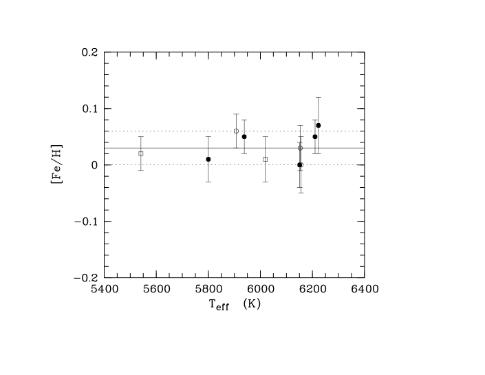
Figure 2: [Fe/H] as a function of effective temperature for the sample stars. Filled and open circles represent main sequence Li-rich and Li-poor stars, while open squares denote the two slightly evolved stars. Error bars shown in the figure correspond to rms values quoted in Table 1. Internal errors due to uncertainties in stellar parameters are not shown here. The solid and dotted lines represent the average [Fe/H] value $\pm 1$ standard deviation.

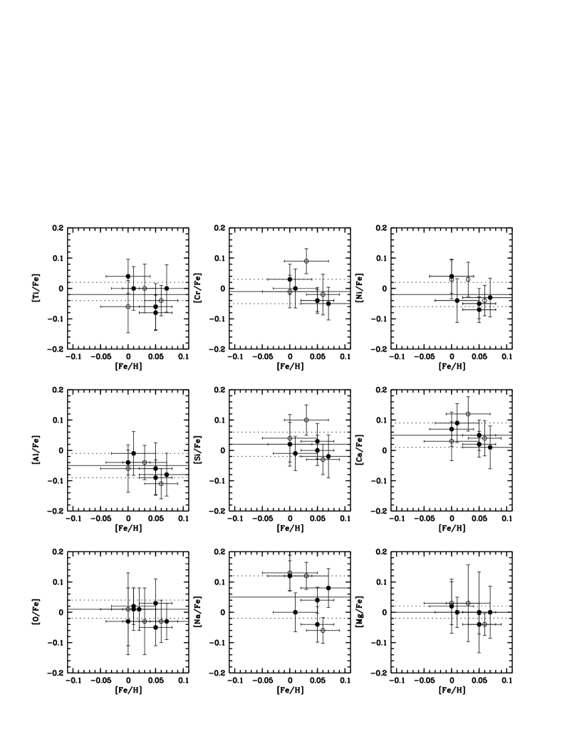
Figure 4: [X/Fe] vs. [Fe/H] for Li-poor (open circles) and Li-rich (filled circles) stars. Error bars in [Fe/H] and [X/Fe] are the same as in Figs. 2 and 3. Horizontal lines are the same as in Fig. 3. The two evolved stars are not plotted in the figure (see text).

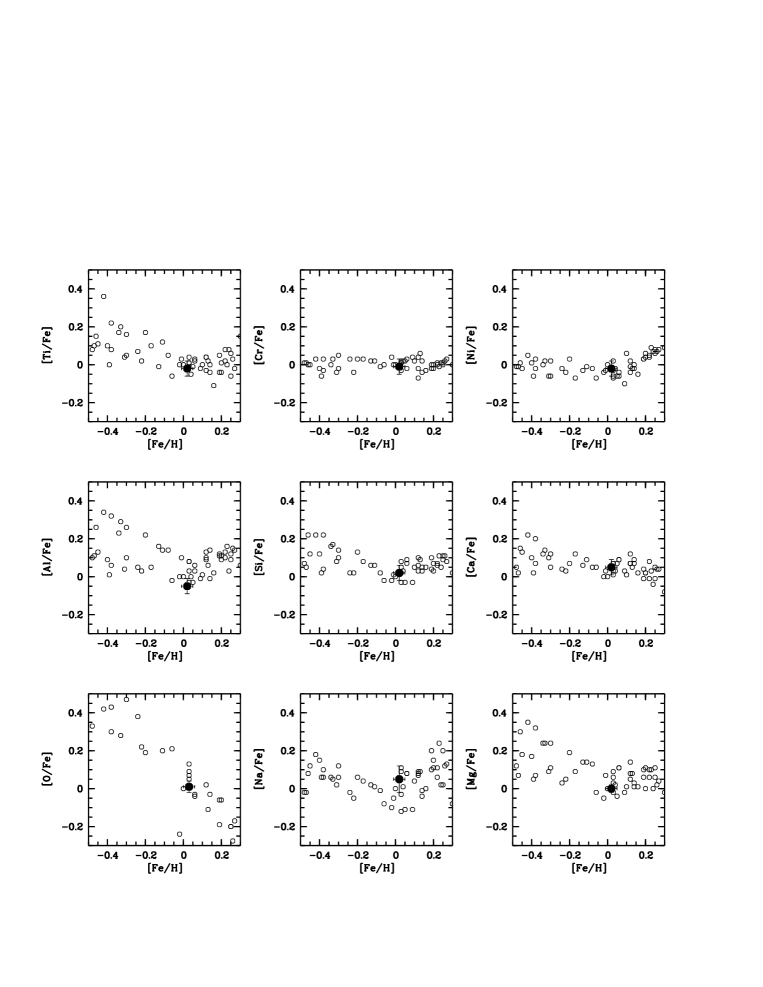
Figure 5: [X/Fe] vs. [Fe/H] for field stars from Bensby et al. (bfl03 (2003), bensby04 (2004) —open circles) and the average values from this study (filled symbols).

[x]lcccr Line list, adopted $\log$ gf values, and solar EWs. (1): VALD; (2): Lambert & Walner (lw (1968)); (3): Chen et al. (chen (2000)); (4): Bensby et al. (bfl03 (2003)); (5): Clementini et al. (clem (1995)); (6): Fulbright (full (2000)); (7): Biémont et al (bie91 (1991)); (*): inverse solar analysis.
Element $\lambda$ (Å) $\log$ gf ref. EW_⊙ (mÅ)
continued.
Element $\lambda$ (Å) $\log$ gf ref. EW_⊙ (mÅ)
O i 6300.633 $-$9.717 (1) 5.5
Na i 5682.633 $-$0.700 (1) 107.0
Na i 5688.220 $-$0.400 (2) 130.0
Na i 6154.226 $-$1.570 (2) 35.0
Na i 6160.747 $-$1.270 (2) 52.9
Mg i 5528.405 $-$0.620 (1) 233.0
Mg i 5711.090 $-$1.724 (3) 105.0
Al i 5557.070 $-$2.160 (*) 11.5
Al i 6696.023 $-$1.540 (*) 39.3
Al i 6698.673 $-$1.890 (*) 20.1
Si i 5701.104 $-$2.050 (1) 37.2
Si i 5948.541 $-$1.230 (1) 81.5
Si i 6091.919 $-$1.400 (1) 30.6
Si i 6125.021 $-$1.550 (*) 30.9
Si i 6142.483 $-$1.480 (6) 33.2
Si i 6145.016 $-$1.440 (5) 37.5
Si i 6414.980 $-$1.100 (1) 46.0
Si i 6518.733 $-$1.500 (1) 20.5
Si i 6555.463 $-$1.000 (1) 43.6
Ca i 5512.980 $-$0.480 (*) 87.0
Ca i 5581.965 $-$0.671 (3) 94.3
Ca i 5601.277 $-$0.523 (3) 105.5
Ca i 5867.562 $-$1.610 (*) 24.4
Ca i 6102.723 $-$0.862 (1) 126.5
Ca i 6122.217 $-$0.386 (1) 171.2
Ca i 6161.297 $-$1.293 (1) 60.5
Ca i 6166.439 $-$1.156 (1) 68.6
Ca i 6169.042 $-$0.804 (1) 87.0
Ca i 6169.563 $-$0.527 (1) 107.6
Ca i 6455.598 $-$1.400 (*) 56.6
Ca i 6499.650 $-$0.818 (3) 87.0
Ti i 4805.415 0.150 (1) 32.6
Ti i 4820.411 $-$0.441 (1) 44.9
Ti i 4885.079 0.358 (1) 64.0
Ti i 4913.614 0.160 (1) 53.7
Ti i 5016.161 $-$0.574 (1) 67.5
Ti i 5219.702 $-$2.292 (1) 28.1
Ti i 5866.451 $-$0.840 (1) 48.1
Ti i 5953.160 $-$0.329 (1) 33.6
Ti i 5965.828 $-$0.409 (1) 29.9
Ti i 6258.102 $-$0.431 (3) 50.9
Ti i 6261.098 $-$0.479 (1) 49.8
Cr i 4936.335 $-$0.340 (1) 42.0
Cr i 5247.566 $-$1.640 (1) 81.2
Cr i 5296.691 $-$1.400 (1) 92.2
Cr i 5300.744 $-$2.120 (1) 59.8
Cr i 5329.142 $-$0.064 (1) 66.0
Cr i 5348.312 $-$1.290 (1) 96.9
Fe i 4835.868 $-$1.500 (1) 46.6
Fe i 4875.878 $-$2.020 (1) 55.6
Fe i 4907.732 $-$1.840 (1) 58.7
Fe i 4999.113 $-$1.740 (1) 31.2
Fe i 5036.922 $-$3.068 (1) 22.2
Fe i 5044.211 $-$2.038 (1) 75.1
Fe i 5067.150 $-$0.970 (1) 70.0
Fe i 5141.739 $-$2.190 (1) 88.8
Fe i 5162.273 0.020 (1) 138.1
Fe i 5217.389 $-$1.070 (1) 110.9
Fe i 5228.377 $-$1.290 (1) 52.1
Fe i 5285.129 $-$1.640 (1) 26.7
Fe i 5293.959 $-$1.870 (1) 29.0
Fe i 5373.709 $-$0.860 (1) 63.0
Fe i 5386.334 $-$1.770 (1) 32.0
Fe i 5397.618 $-$2.480 (1) 23.1
Fe i 5472.709 $-$1.495 (1) 42.8
Fe i 5522.447 $-$1.550 (1) 41.4
Fe i 5539.280 $-$2.660 (1) 16.2
Fe i 5543.150 $-$1.570 (1) 63.3
Fe i 5543.936 $-$1.140 (1) 60.2
Fe i 5546.992 $-$1.910 (1) 23.9
Fe i 5584.765 $-$2.320 (1) 34.8
Fe i 5636.696 $-$2.610 (1) 19.1
Fe i 5638.262 $-$0.870 (1) 73.8
Fe i 5662.516 $-$0.573 (1) 93.4
Fe i 5691.497 $-$1.520 (1) 39.6
Fe i 5701.545 $-$2.216 (1) 84.8
Fe i 5862.353 $-$0.058 (1) 86.4
Fe i 5916.247 $-$2.994 (1) 54.2
Fe i 5930.180 $-$0.230 (1) 88.8
Fe i 5934.655 $-$1.170 (1) 72.6
Fe i 5956.694 $-$4.605 (1) 54.1
Fe i 5976.775 $-$1.310 (1) 66.7
Fe i 5984.814 $-$0.343 (1) 82.7
Fe i 5987.066 $-$0.556 (1) 66.8
Fe i 6003.012 $-$1.120 (1) 77.8
Fe i 6024.058 $-$0.120 (1) 108.7
Fe i 6056.005 $-$0.460 (1) 72.6
Fe i 6078.491 $-$0.424 (1) 76.0
Fe i 6136.995 $-$2.950 (1) 68.6
Fe i 6157.728 $-$1.260 (1) 61.8
Fe i 6187.990 $-$1.720 (1) 46.2
Fe i 6200.313 $-$2.437 (1) 73.5
Fe i 6315.811 $-$1.710 (1) 40.3
Fe i 6322.685 $-$2.426 (1) 75.0
Fe i 6336.824 $-$0.856 (1) 105.5
Fe i 6344.149 $-$2.923 (1) 61.0
Fe i 6469.193 $-$0.770 (1) 54.8
Fe i 6495.742 $-$0.940 (1) 42.2
Fe i 6498.939 $-$4.699 (1) 46.6
Fe i 6574.228 $-$5.023 (1) 29.4
Fe i 6609.110 $-$2.692 (1) 66.2
Fe i 6703.567 $-$3.160 (1) 38.1
Fe i 6733.151 $-$1.580 (1) 23.1
Fe i 6750.153 $-$2.621 (1) 74.2
Fe i 6806.845 $-$3.210 (1) 33.7
Fe ii 5264.812 $-$3.120 (1) 47.1
Fe ii 5325.553 $-$3.222 (7) 41.1
Fe ii 5414.073 $-$3.750 (7) 23.7
Fe ii 5425.257 $-$3.372 (7) 37.8
Fe ii 5991.376 $-$3.557 (7) 31.4
Fe ii 6084.111 $-$3.808 (7) 21.5
Fe ii 6149.258 $-$2.724 (7) 34.8
Fe ii 6247.557 $-$2.329 (7) 53.6
Fe ii 6432.680 $-$3.708 (7) 39.4
Fe ii 6456.383 $-$2.075 (7) 64.4
Fe ii 6516.080 $-$3.450 (7) 49.3
Ni i 4806.984 $-$0.640 (1) 59.2
Ni i 4852.547 $-$1.070 (1) 42.7
Ni i 4904.407 $-$0.170 (1) 87.9
Ni i 4913.968 $-$0.630 (1) 58.7
Ni i 4946.029 $-$1.290 (1) 23.5
Ni i 5003.734 $-$3.130 (4) 32.8
Ni i 5010.934 $-$0.870 (1) 52.2
Ni i 5032.723 $-$1.270 (1) 20.6
Ni i 5082.339 $-$0.590 (*) 62.8
Ni i 5155.125 $-$0.650 (1) 47.9
Ni i 5435.855 $-$2.590 (1) 45.8
Ni i 5462.485 $-$0.930 (1) 39.9
Ni i 5589.357 $-$1.140 (1) 27.1
Ni i 5593.733 $-$0.840 (1) 41.6
Ni i 5625.312 $-$0.700 (1) 38.6
Ni i 5641.880 $-$1.070 (1) 24.1
Ni i 5682.198 $-$0.499 (3) 50.1
Ni i 6111.066 $-$0.870 (1) 33.4
Ni i 6175.360 $-$0.559 (1) 48.4
Ni i 6186.709 $-$0.960 (1) 29.0
Ni i 6191.171 $-$2.353 (1) 74.9
Ni i 6223.981 $-$0.910 (1) 26.2
Ni i 6378.247 $-$0.830 (1) 33.3
Ni i 6586.308 $-$2.810 (1) 41.0