Capturing Halos at High Redshifts

Abstract

We study the evolution of the mass function of dark matter halos in the concordance $\Lambda$CDM model at high redshift. We employ overlapping (multiple-realization) numerical simulations to cover a wide range of halo masses, $10^{7}-10^{15}h^{-1}M_{\odot}$, with redshift coverage beginning at $z=20$. The Press-Schechter mass function is significantly discrepant from the simulation results at high redshifts. Of the more recently proposed mass functions, our results are in best agreement with Warren et al. (2005). The statistics of the simulations – along with good control over systematics – allow for fits accurate to the level of $20\%$ at all redshifts. We provide a concise discussion of various issues in defining and computing the halo mass function, and how these are addressed in our simulations.

                                                                                                                                     LA-UR-05-9198

1 Introduction

Dark matter halos occupy a central place in the paradigm of gravitationally-driven structure formation arising from the nonlinear evolution of primordial Gaussian density fluctuations. Gas condensation, resultant star formation, and eventual galaxy formation occurs within halos. Consequently, the halo profile and mass function are central ingredients in phenomenological models of nonlinear clustering of galaxies. The distribution of halo masses – the halo mass function – and its time evolution, are also sensitive probes of cosmology.

The halo mass function at the high-mass end (cluster mass scales) is exponentially sensitive to the amplitude of the initial density perturbations, the mean matter density parameter, $\Omega_{m}$, and to the dark energy controlled late-time evolution of the density field. The last feature, particularly at low redshifts, $z<2$, allows cluster observations to constrain the dark energy content, $\Omega_{\Lambda}$, and the equation of state parameter, $w$ Holder et al. (2001).

The halo mass function is also of considerable interest at high redshift, relating to questions such as predictions for quasar abundance and formation sites Haiman & Loeb (2001), the formation history of collapsed baryonic halos, and the reionization history of the Universe Furlanetto et al. (2005). Recent results from the Wilkinson Microwave Anisotropy Probe (WMAP) (Kogut et al. 2003; Spergel et al. 2003) indicate that reionization could have begun at redshifts as high as $z\sim 20$. Much of the work on possible reionization scenarios is based on the simple Press-Schechter (PS) mass function (Press & Schechter 1974, Bond et al. 1991) the use of which can lead to imprecise predictions for the reionization history.

Simulations play a dual role in characterization of the halo mass function. If only a few fixed sets of cosmological parameters and a finite dynamic range are required, simulations can produce valuable results. In order to investigate a variety of cosmologies and different scenarios for physical processes, e.g., reionization, it is nevertheless very convenient, if not necessary, to have accurate analytic fitting relations. Simulations can be used to validate these fits over a wide (albeit, discretely sampled) range of parameters.

Various numerical studies of the mass function have been carried out over different mass and redshift ranges. The closest to the present work are Reed et al. (2003) and Springel et al. (2005); in comparison to their results, our halo mass range goes deeper by three orders of magnitude, with good statistics and control of systematics out to $z=20$, substantially higher than in these papers. (We review results from other work below.) Essentially, the earlier results are in very good agreement with the Sheth-Tormen mass function Sheth & Tormen (1999), at redshifts $z\leq 10$. As we show below, various fitting formulae given in the literature – most tuned to simulation results at $z=0$ – can differ substantially in their predictions at high redshifts, by as much as a factor of two. Therefore, it is important to carry out simulations of sufficient dynamic range and accuracy to test these predictions.

In order to extract the mass function from simulations, different questions have to be addressed, such as: How is the mass function to be defined? When do the first halos form in a simulation? When must the simulation be started in order to capture these halos? What force and mass resolution is required to capture halos of a certain mass at a specific redshift? We have derived and tested certain criteria to ensure that our simulations capture the halos of interest; details will be given elsewhere Lukić et al. (2006).

The paper is organized as follows. In Section 2 we discuss popular mass function formulae, previous work, and strategies for determining the halo mass function at high redshifts. The simulations and mass function results are discussed in Section 3. Criteria for mass and force resolution and initial redshift needed to span the desired mass and redshift range are given here. We present our conclusions in Section 4.

2 The Mass Function

Over the last three decades different fitting functions for the mass function have been suggested. The first analytic model for the mass function was developed by Press & Schechter (1974). Their theory considers a spherically overdense region in an otherwise smooth background density field. The overdensity evolves as a Friedmann universe with positive curvature. Initially, the overdensity expands, but at a slower rate than the background universe (thus enhancing the density contrast), until it reaches the ‘turnaround’ density, after which it collapses. Although formally this collapse ends with a singularity, it is assumed that in reality the overdense region will virialize. For an Einstein-de Sitter universe, the density of such an overdense region at the virialization redshift is $\rho\approx 180\rho_{c}(z)$. At this point, the density contrast from the linear theory of perturbation growth [$\delta(\vec{x},z)=D^{+}(z)\delta(\vec{x},0)$] is $\delta_{c}(z)\approx 1.686(1+z)$. For $\Omega_{m}<1$, $\delta_{c}(z)$ evolves differently (see Lacey & Cole 1993), but the dependence on cosmology is weak (see e.g., Jenkins et al. 2001). Thus, we adopt $\delta_{c}=1.686=\delta_{c}(0)$.

Following the above reasoning and with the assumption that the initial density perturbations are given by a Gaussian random field, the PS mass function is given by:

$$f_{PS}(\sigma)=\sqrt{\frac{2}{\pi}}\frac{\delta_{c}}{\sigma}\exp\left[-\frac{\delta^{2}_{c}}{2\sigma^{2}}\right],$$ (1)

where $\sigma$ is the variance of the linear density field, $f(\sigma,z)\equiv(M/\rho_{b})(dn/d\ln\sigma^{-1})$, and $\rho_{b}$ is the background density.

Using empirical arguments Sheth & Tormen (1999, hereafter ST) proposed an improved fit of the following form:

$$f_{ST}(\sigma)=0.3222\sqrt{\frac{2a}{\pi}}\frac{\delta_{c}}{\sigma}\exp\left[-\frac{a\delta^{2}_{c}}{2\sigma^{2}}\right]\left[1+\left(\frac{\sigma^{2}}{a\delta^{2}_{c}}\right)^{p}\right],$$ (2)

with $a=0.707$, and $p=0.3$. Sheth et al. (2001) interpreted this fit theoretically by extending the PS approach to an ellipsoidal collapse model. In this model, the collapse of a region depends not only on its initial overdensity, but also on the surrounding shear field. The dependence is chosen to recover the Zel’dovich approximation Zel’dovich (1970) in the linear regime. A halo is considered virialized when the third axis collapses (see also Lee & Shandarin 1997).

Jenkins et al. (2001, hereafter Jenkins) combine high resolution simulations for different cosmologies spanning a mass range of over three orders of magnitude [$\sim(10^{12}-10^{15})h^{-1}M_{\sun}$], and including several redshifts between $z=5$ and $z=0$. They find that the following fitting formula works exceptionally well (within 20%), independent of the underlying cosmology:

$$f_{Jenkins}(\sigma)=0.315\exp\left[-|\ln\sigma^{-1}+0.61|^{3.8}\right].$$ (3)

The above formula is very close to the nominal ST fit.

By performing 16 nested-volume simulations Warren et al. (2005, hereafter Warren) obtain significant halo statistics spanning a mass range of five orders of magnitude [$\sim(10^{10}-10^{15})h^{-1}M_{\sun}$]. Their best fit employs a functional form similar to an improved version of ST (Sheth & Tormen 2002):

$$f_{Warren}(\sigma)=0.7234\left(\sigma^{-1.625}+0.2538\right)\exp\left[-\frac{1.1982}{\sigma^{2}}\right].$$ (4)

The discrepancy between PS and the more accurate fits is evident in Figure 1 where the redshift evolution of the mass function is shown. The redshift dependence in the analytic mass functions enters only through $\sigma(z)=\sigma(0)d(z)$, where $d(z)$ is the growth factor normalized such that $d(0)=1$. As the functional dependence on $\sigma$ is different in the different fits, this leads to substantial variation across the fits as a function of redshift. For $z=0$ the Warren fit agrees – especially in the low mass range below $10^{13}M_{\odot}$ – to better than 5% with the ST fit. At the high mass end the difference increases up to 20%. The Jenkins fit leads to similar results over the considered mass range. Note that at higher redshifts and intermediate mass ranges around $10^{9}M_{\odot}$ the disagreement between the Warren and ST fits increases up to 40%.

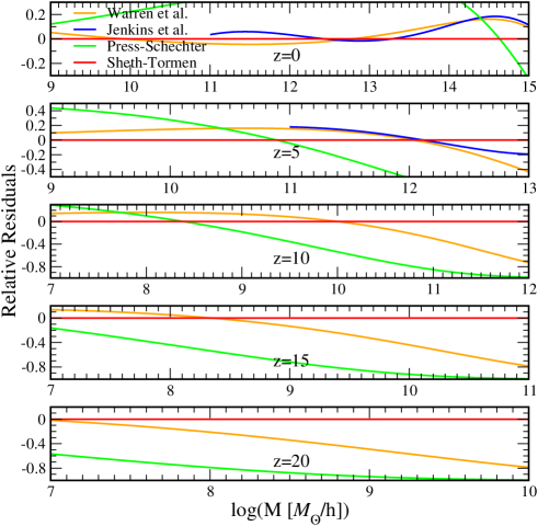
Figure 1: Relative residuals of the PS, Jenkins, and Warren mass function fits with respect to ST for five different redshifts. Note that the ranges of the axes are different in the different panels. We do not show the Jenkins fit below masses of 10${}^{11}h^{-1}M_{\odot}$ since it is not valid in this mass range.

The determination of mass functions at high redshifts is a nontrivial task. High redshift halos have very low masses, placing heavy demands on the mass and force resolution needed to resolve them. These requirements can be achieved in two ways. First, a simulation with a very large number of particles and high force resolution can be performed. This is expensive, and only a very limited number of such simulations can be carried out. Second, since determining the mass function is simply a question of statistics, many relatively modest simulations with moderate particle loading can be performed: this is the strategy we adopt here. As simulations can only be trusted until a redshift at which the largest mode is close to becoming nonlinear, multiple overlapping box sizes must be used.

Springel et al. (2005) have recently followed the evolution of 2160³ particles in a $500h^{-1}$Mpc box. The high mass and force resolution allow them to study the mass function reliably out to a redshift of $z=10$, covering a mass range of roughly $10^{10}h^{-1}M_{\odot}$ to $10^{16}h^{-1}M_{\odot}$. Examples of single small-box simulations include Jang-Condell & Hernquist (2001) (1$h^{-1}$Mpc box with $128^{3}$ particles evolved to $z=10$) and Cen et al. (2004) ($4h^{-1}$Mpc box, $512^{3}$ particles, evolved to $z=6$). Results in both papers are claimed to be consistent with PS but without detailed quantification. The simulation of Reed et al. (2003) is a compromise between the two extremes: a box size of 50$h^{-1}$Mpc with 432³ particles and a concomitant halo mass range of roughly 10${}^{10}h^{-1}M_{\odot}$ to $10^{14.5}h^{-1}M_{\odot}$. Reed et al. find good agreement (better than 20%) with the ST fit up to $z\simeq 10$. For higher redshifts they find that the ST fit overpredicts the number of halos, at $z=15$ up to 50%. At this high redshift, however, their results become statistics-limited, the mass resolution being insufficient to resolve the very small halos.

In this paper we analyze a suite of 50 N-body simulations with varying box sizes between $4h^{-1}$Mpc and $126h^{-1}$Mpc with multiple realizations of all boxes to study the mass function at redshifts up to $z=20$ and to cover a large mass range between $10^{7}h^{-1}M_{\odot}$ and $10^{15}h^{-1}M_{\odot}$ even at high redshifts. Significantly, at $z=20$, gas in halos with a mass scale above $\sim 10^{7}h^{-1}M_{\odot}$ can cool via atomic line cooling Tegmark et al. (1997).

3 Simulations and Mass Function Results

Table 1: Summary of the performed runs

Mesh	Box Size	Resolution	$z_{in}$	$z_{final}$	Particle Mass	Smallest Halo	# of Realizations
10243	126 $h^{-1}$Mpc	120 $h^{-1}$kpc	50	0	$9.94\times 10^{9}~{}h^{-1}M_{\odot}$	$3.98\times 10^{11}~{}h^{-1}M_{\odot}$	10
10243	64 $h^{-1}$Mpc	62.5 $h^{-1}$kpc	80	0	$1.30\times 10^{9}~{}h^{-1}M_{\odot}$	$5.2\times 10^{10}~{}h^{-1}M_{\odot}$	5
10243	32 $h^{-1}$Mpc	31.25 $h^{-1}$kpc	150	5	$1.63\times 10^{8}~{}h^{-1}M_{\odot}$	$6.52\times 10^{9}~{}h^{-1}M_{\odot}$	5
10243	16 $h^{-1}$Mpc	15.63 $h^{-1}$kpc	200	5	$2.04\times 10^{7}~{}h^{-1}M_{\odot}$	$8.16\times 10^{8}~{}h^{-1}M_{\odot}$	5
10243	8 $h^{-1}$Mpc	7.81 $h^{-1}$kpc	250	10	$2.55\times 10^{6}~{}h^{-1}M_{\odot}$	$1.02\times 10^{8}~{}h^{-1}M_{\odot}$	20
10243	4 $h^{-1}$Mpc	3.91 $h^{-1}$kpc	500	10	$3.19\times 10^{5}~{}h^{-1}M_{\odot}$	$1.27\times 10^{7}~{}h^{-1}M_{\odot}$	5

All simulations in this paper are carried out with the particle-mesh code MC² (Mesh-based Cosmology Code). MC² has been extensively tested against other cosmological simulation codes (Heitmann et al. 2005). The chosen values of cosmological parameters are:

$$\Omega_{\rm tot}=1.0,~{}~{}~{}\Omega_{m}=0.253,~{}~{}~{}\Omega_{\rm baryon}=0.048,$$

$$\sigma_{8}=0.9,~{}~{}~{}H_{0}=70~{}{\rm km/s/Mpc},$$ (5)

as set by the latest cosmic microwave background and large scale structure observations MacTavish et al. (2005). The mass transfer functions are generated with CMBFAST (Seljak & Zaldarriaga 1996). We summarize the different runs, including their force and mass resolution in Table 1.

We identify halos with the friends-of-friends algorithm (FOF), based on finding neighbors of particles at a certain distance (see e.g., Einasto et al. 1984; Davis et al. 1985). The halo mass is defined simply by the sum of particles which are members of the halo. (For connections between different definitions of halo masses, see White 2001.) Despite several shortcomings of the FOF halo finder, e.g., halo-bridging (see, e.g., Gelb & Bertschinger 1994, Summers et al. 1995) or statistical biases found by Warren et al. (2005), the FOF algorithm itself is well-defined and very fast.

There are two sources of possible biases in determining individual halo masses using FOF. First, the halo may be sampled with an insufficient number of particles (see Warren et al. 2005). Second, the effective slope of the halo density profile close to the virial radius $r_{vir}$, at fixed particle number, also influences the FOF mass. If the force resolution of the N-body code affects the profile, this too, adds a systematic bias. Here we record the mass function for the linking length $b=0.2$ FOF mass including only the correction of Warren et al. (2005). In a follow-up paper (Lukić et al. 2006) we will address systematics issues in determining halo masses in detail.

We now discuss criteria found to be very important for demonstrating the convergence and robustness of our results. Details will be presented in Lukić et al. (2006). The first issue relates to the initial redshift of the simulation. Two conditions are important: (i) the simulation must begin sufficiently early that the initial Zel’dovich displacement is a small enough fraction of the mean interparticle separation $\Delta_{p}$; on average a particle should not move more than $\sim\Delta_{p}/3$; (ii) the highest redshift where the mass function is to be evaluated must be sufficiently removed from the redshift of first-crossing $z_{cross}$ where particles have the first chance to form halos. The stringency of these criteria is such that the small boxes require very high starting redshifts, e.g., the 4$h^{-1}$Mpc box had an initial redshift $z_{in}=500$. This is a much earlier starting redshift than those used in previous simulations; the conventional requirement that all modes in the box be linear at the initial redshift proves to be much weaker, and therefore inadequate, as a convergence criterion.

A simple test of how well the simulations track the mass function formulae is to follow the number of halos in a specified mass bin at a given redshift. For this purpose we convert the mass function fit into a function of $z$, defining the halo growth function as shown in Figure 2. The evolution of three mass bins is shown as a function of $z$ along with results from the $16h^{-1}$Mpc boxes. The halo growth function is particularly valuable for determining when the halos at a certain mass should first form. This is a good test for problems in simulations aiming to capture halos with a given minimum mass at some redshift. An example of this is insufficient force resolution in the base-grids of adaptive-mesh-refinement (AMR) codes.

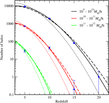
Figure 2: Halo growth function for three mass bins for the 16$h^{-1}$Mpc box. The Warren (solid), ST (long-dashed), and PS (short-dashed) fits are compared to simulation data with Poisson error bars. Note the quality of the agreement with the Warren fit.

Once the number of particles for a simulation and a desired mass for the smallest halo are decided, the required box size is fixed. The force resolution needed to resolve the smallest halos has then to be determined. Our aim here is not to precisely measure the halo profile but simply to be certain that the total halo mass is correct. As shown in Heitmann et al. (2005) the halo mass is a relatively robust quantity and a simple estimate of the force resolution is all that is needed. The force resolution must be small compared to the comoving halo virial radius $r_{\Delta}$ (with the overdensity relative to the critical density, $\Delta\sim 200$) at all redshifts. The resulting inequality can be stated in the form

$$\frac{\delta_{f}}{\Delta_{p}}<0.62\left(\frac{n_{h}\Omega(z)}{\Delta}\right)^{1/3},$$ (6)

where $\delta_{f}$ is the force resolution and $n_{h}$ is the number of particles per halo. In the simulations performed here we use a ratio of one particle per 64 grid cells, which allows halos with roughly 50 particles to be captured. It has been shown in Heitmann et al. (2005) that this ratio does not cause collisional effects and leads to consistent results in comparison with other codes. Mass function convergence tests with different force resolutions are nicely consistent with the above estimate as shown in Lukić et al. (2006); time-step criteria and convergence tests are also described there.

The large set of simulations we have carried out allows us to study the mass function at redshifts between $z=20$ and $z=0$. The main results are shown in Figure 3, where the simulation data for the mass function are shown along with the Warren, PS, and ST fits at different redshifts. At all redshifts the Warren fit has the best agreement with the simulations with a scatter of approximately $20\%$ and is a numerically significant improvement over ST. Such a close match is quite gratifying given the overall dynamic range of the investigation. The PS fit, over the mass range considered, is a poor fit at $z\geq 10$, deviating by more than a factor of two from the numerical results.

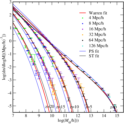
Figure 3: The mass function at 5 different redshifts with Poisson error bars. The red line is the Warren fit, blue is Press-Schechter, and black is Sheth-Tormen.

4 Conclusions and Discussion

In this paper we have studied the evolution of the mass function starting at a redshift of $z=20$ and covering a halo mass range of $10^{7}$ to $10^{15}h^{-1}M_{\odot}$. Our results incorporate new halo-based N-body error control criteria that are described in more detail in Lukić et al. (2006). We find that the Press-Schechter mass function deviates significantly from our results. More recent mass function fits are in better agreement; in particular, the recently introduced fitting function of Warren et al. (2005) agrees at the $20\%$ level over the entire redshift range.

The precise agreement of the numerically obtained halo growth function as well as the evolution of the mass function with the (evolved $z=0$) Warren fit demonstrates the remarkable result that the evolution of the mass function is completely controlled by the linear growth of the variance of the linear density field.

In order to find a mass function fit relevant to observations, several hurdles remain to be overcome, including reaching agreement on an appropriate definition of halo mass (White 2001) and improving the precision and accuracy of N-body codes beyond the current state of the art (O’Shea et al. 2005; Heitmann et al. 2005). Depending on the level of precision required, as White (2002) points out, “it may not be sufficient to use a simple parametrized form” in constraining cosmological parameters with the mass function.

The error control criteria developed in this work have a natural application in high-resolution AMR simulations in the setting of refinement and error control criteria. Work in this direction is in progress.

References

- Bond et al. (1991) Bond, J.R, Cole, S., Efstathiou, G, Kaiser, N. 1991, ApJ, 379, 440
- Cen et al. (2004) Cen, R., Dong, F., Bode, P., & Ostriker, J.P. 2004, astro-ph/0403352, ApJ, submitted
- Davis et al. (1985) Davis, M., Efstathiou, G., Frenk, C.S. 1985, ApJ, 292, 371
- Einasto et al. (1984) Einasto, J., Klypin, A.A., Saar, E., Shandarin, S.F. 1984, MNRAS, 206, 529
- Furlanetto et al. (2005) Furlanetto, S.R., McQuinn, M., Hernquist, L., 2005 astro-ph/0507524
- Gelb & Bertschinger (1994) Gelb, J.M. & Bertschinger, E. 1994, ApJ, 436, 467
- Haiman & Loeb (2001) Haiman, Z., Loeb, A. 2001, ApJ, 552, 459
- Heitmann et al. (2005) Heitmann, K., Ricker, P.M., Warren, M.S., & Habib, S. 2005, ApJS, 160, 28
- Holder et al. (2001) Holder, G, Haiman, Z., & Mohr, J. ApJ, 560, L111
- Jang-Condell & Hernquist (2001) Jang-Condell, H. & Hernquist, L. 2001, ApJ, 548, 68
- Jenkins et al. (2001) Jenkins, A. et al. 2001, MNRAS, 321, 372
- Kogut et al. (2003) Kogut, A. et al. 2003, ApJS, 148, 161
- Lacey & Cole (1993) Lacey, C.G. & Cole, S. 1993, MNRAS, 262, 627
- Lukić et al. (2006) Lukić, Z., Heitmann, K., Habib, S., & Ricker, P.M. 2006, in preparation
- MacTavish et al. (2005) MacTavish, C.J. et al. 2005, astro-ph/0507503, ApJ, submitted
- O’Shea et al. (2005) O’Shea, B.W., Nagamine, K., Springel, V., Hernquist L., & Norman, M.L. 2005, ApJS, 160, 1
- Press & Schechter (1974) Press, W.H. & Schechter, P. 1974, ApJ, 187, 425
- Reed et al. (2003) Reed, D. et al. 2003, MNRAS, 346, 565
- Seljak & Zaldarriaga (1996) Seljak, U. & Zaldarriga, M. 1996, ApJ, 469, 437
- Sheth & Tormen (1999) Sheth, R.K. & Tormen, G. 1999, MNRAS, 308, 119
- Sheth & Tormen (2002) Sheth, R.K. & Tormen, G. 2002, MNRAS, 329, 61
- Sheth et al. (2001) Sheth, R.K., Mo, H.J., & Tormen, G. 2001, MNRAS, 323, 1
- Spergel et al. (2003) Spergel, D.N. et al. 2003, ApJS, 148, 175
- Springel et al. (2005) Springel, V. et al. 2005, Nature, 435, 629
- Summers et al. (1995) Summers, F.J., Davis, M. & Evrard, A.E. 1995, ApJ, 454, 1
- Tegmark et al. (1997) Tegmark, M. et al. 1997, ApJ, 474, 1
- Warren et al. (2005) Warren, M.S., Abazajian, K., Holz, D.E., and Teodoro, L. 2005, ApJL, submitted
- White (2001) White, M. 2001, A&A, 367, 27
- White (2002) White, M. 2002, ApJS, 143, 241
- Zel’dovich (1970) Zel’dovich, Y.B. 1970, A& A, 5, 84