Lyman break galaxies, Ly$\alpha$ emitters and a radio galaxy in a protocluster at $z=4.1$ .

Abstract

We present deep HST/ACS observations in $g_{475}$$r_{625}$$i_{775}$$z_{850}$ towards the $z=4.1$ radio galaxy TN J1338–1942 and its overdensity of $>$30 spectroscopically confirmed Ly$\alpha$ emitters (LAEs). We select 66 $g_{475}$-band dropouts to $z_{850}$${}_{,5\sigma}=27$, 6 of which are also a LAE. Although our color-color selection results in a relatively broad redshift range centered on $z=4.1$, the field of TN J1338–1942 is richer than the average field at the $>$5$\sigma$ significance, based on a comparison with GOODS. The angular distribution is filamentary with about half of the objects clustered near the radio galaxy, and a small, excess signal ($2\sigma$) in the projected pair counts at separations of $\theta<10\arcsec$ is interpreted as being due to physical pairs. The LAEs are young (a few $\times 10^{7}$ yr), small ($\langle r_{hl}\rangle=0\farcs 13$) galaxies, and we derive a mean stellar mass of $\sim 10^{8-9}$ M_⊙ based on a stacked $K_{S}$-band image. We determine star formation rates, sizes, morphologies, and color-magnitude relations of the $g_{475}$-dropouts and find no evidence for a difference between galaxies near TN J1338–1942 and in the field. We conclude that environmental trends as observed in clusters at much lower redshift are either not yet present, or are washed out by the relatively broad selection in redshift. The large galaxy overdensity, its corresponding mass overdensity and the sub-clustering at the approximate redshift of TN J1338–1942 suggest the assemblage of a $>10^{14}$ M_⊙ structure, confirming that it is possible to find and study cluster progenitors in the linear regime at $z\gtrsim 4$.

1. Introduction

The formation and evolution of structure in the Universe is a fundamental field of research in cosmology. Clusters of galaxies represent the most extreme deviation from initial conditions in the Universe, and are therefore good evolutionary probes for studying the formation of the large-scale structure. While clusters of galaxies have been studied extensively in the relatively nearby Universe, their evolutionary history becomes obscure beyond roughly half the Hubble time (Blakeslee et al., 2006; Mullis et al., 2005; Stanford et al., 2006). Their progenitors are extremely difficult to identify when the density contrast between the forming cluster and the field becomes small, and mass condensations on the scales of clusters are extremely rare at any epoch (Kaiser, 1984).

Even the most distant clusters known contain, besides a population of star-forming galaxies, an older population of relatively red and massive galaxies (e.g. Dressler et al., 1999; van Dokkum et al., 2000; Goto et al., 2005). The scatter in the color-magnitude relation for cluster ellipticals at $z\sim 1$ is virtually indistinguishable from that at low redshift, suggesting that some of the galaxy populations in clusters have very old stellar populations (e.g. Stanford et al., 1998; Blakeslee et al., 2003; Wuyts et al., 2004; Holden et al., 2005). The epoch of cluster and cluster galaxy formation is presumed to be marked by the violent build-up of the stellar mass and morphologies of these early-type galaxies.

Large samples of star-forming Lyman break galaxies (LBGs) that are selected in the rest-frame UV have been used to probe the cosmic star formation rate history as well as the large-scale structure far beyond $z=1$. The epoch corresponding to the peak in the star formation rate density ($z\sim 2-3$) is preceded by a significant but modest decrease in the star formation rate density from $z\sim 3$ out to $z\sim 6$ (Madau et al., 1996; Steidel et al., 1999; Giavalisco et al., 2004a; Bouwens et al., 2007). Deep near-IR NICMOS observations in and around the GOODS fields find small samples of $z\sim 7-8$ galaxies (Bouwens & Illingworth, 2006; Bouwens et al., 2004c) and indicate that this decline in the number of $UV$ luminous galaxies continues from $z\sim 7-8$ (Bouwens & Illingworth, 2006). This suggests that cosmic star formation is a rather extended process, with only modest but continual changes over time.

LBGs, as well as the partially overlapping population of Ly$\alpha$ emitters (LAEs), are strongly clustered at $z=3-5$, and are highly biased relative to predictions for the dark matter distribution (Giavalisco et al., 1998; Adelberger et al., 1998; Ouchi et al., 2004b; Lee et al., 2006; Kashikawa et al., 2006). The biasing becomes stronger for galaxies with higher rest-frame UV luminosity (Giavalisco & Dickinson, 2001). Ouchi et al. (2004b) found that the bias may also increase with redshift and dust extinction. They suggest that the reddest LBGs could be connected with sub-mm sources or the extremely red objects (EROs, Elston et al., 1988; McCarthy et al., 2001; Daddi et al., 2002). By comparing the number densities of LBGs to that of dark halos predicted by Sheth & Tormen (1999), they concluded that LBGs at $z\sim 4$ are hosted by halos of $1\times 10^{11}-5\times 10^{12}$ M_⊙, and that the descendants of those halos at $z=0$ have masses that are comparable to the masses of groups and clusters. The derived halo occupation numbers of LBGs increase with luminosity from a few tenths to roughly unity, implying that there is only one-to-one correspondence between halos and LBGs at the highest masses.

Studies of sizes indicate that high-redshift star-forming galaxies are compact in size ($\sim 0.1$″–0.3″), while large ($\gtrsim 0.4$″) low surface brightness galaxies are rare (Bouwens et al., 2004a), and there is a clear decrease in size with redshift for objects of fixed luminosity (Ferguson et al., 2004; Bouwens et al., 2004a). Morphological analysis of LBGs indicates that they often possess brighter nuclei and more disturbed profiles than local Hubble types degraded to the same image quality (e.g. Lotz et al., 2004).

Despite these advances in the study of the evolution of the highest redshift galaxies, galaxy clusters have been studied out to only $z=1.5$ while it is clear that they began forming at much earlier epochs. Finding and studying these cluster progenitors may yield powerful tests for (semi-)analytical models and $N$-body simulations of structure formation, and give new clues to how the most massive structures in the Universe came about.

Several good candidates for galaxy overdensities, possibly ‘protoclusters’, have been discovered at very high redshift (e.g. Pascarelle et al., 1996; Keel et al., 1999; Francis et al., 2001; Möller & Fynbo, 2001; Steidel et al., 1998, 2005; Shimasaku et al., 2003; Ouchi et al., 2005b; Kashikawa et al., 2007). These structures have been found often as by-products of wide field surveys using broad or narrow band imaging.

Luminous radio galaxies have also been used to search for overdense regions within the large-scale structure at high redshift. The association of distant, powerful radio galaxies with massive galaxy and cluster formation is mainly based on two observational clues. First, some high redshift radio galaxies are very massive systems (e.g. De Breuck et al., 2002; Dey et al., 1997; Pentericci et al., 2001; Villar-Martín et al., 2005; Miley et al., 2006; Seymour et al., 2007), suggesting that their host galaxies are likely to be the progenitors of massive red sequence galaxies or even the brightest cluster galaxies (BCGs) that dominate the deep potential wells of clusters. Second, in some cases high redshift radio galaxies have been shown to have companion galaxies. At $1.5<z<2$, there is evidence for overdensities of red galaxies associated with radio sources, consistent with moderately rich Abell-type clusters (e.g. Sánchez & González-Serrano, 1999, 2002; Thompson et al., 2000; Hall et al., 2001; Best et al., 2003; Wold et al., 2003). At $z>2$, several radio galaxies have been found to be surrounded by overdensities of LAEs of a few, discovered through deep narrow band imaging and spectroscopic follow-up with the Very Large Telescope (VLT) of the European Southern Observatory (e.g. Pentericci et al., 2000; Kurk et al., 2003; Venemans et al., 2002, 2004, 2005, 2007).

Focussing on the excesses of LAEs discovered in the vicinity of distant radio sources, we are performing a survey of LBGs in such radio-selected protoclusters with the Advanced Camera for Surveys on the Hubble Space Telescope (HST/ACS; Ford et al., 1998). In Miley et al. (2004) and Overzier et al. (2006a) we reported on the detection of a significant population of LBGs in the (projected) region around radio galaxies at $z=4.1$ (TN J1338–1942) and $z=5.2$ (TN J0924–2201). Here, we will present a detailed analysis of the ACS observations of protocluster TN J1338–1942 at $z=4.1$, augmented by ground-based observations with the VLT. This structure is amongst the handful of overdense regions so far discovered at $z>4$, as evidenced by 37 LAEs that represent a surface overdensity of $\sim 5$ compared to other fields (Venemans et al., 2002, 2007). The FWHM of the velocity distribution of the LAEs is 625 km s^-1. The mass overdensity as well as the velocity structure is consistent with the global properties of $z\sim 4$ protoclusters derived from simulations (e.g. De Lucia et al., 2004; Suwa et al., 2006). The radio galaxy itself is highly luminous in the rest-frame UV, optical and the sub-mm, indicating a high star formation rate. It has a complex morphology which we have interpreted as arising from AGN feedback on the forming ISM and a massive starburst-driven wind (Zirm et al., 2005).

The main issues that we will attempt to address here are the following. What are the star formation histories, physical sizes and morphologies of LAEs and LBGs? In particular we wish to study these properties in relation to the overdense environment that the TN J1338–1942 field is believed to be associated with, analogous to galaxy environmental dependencies observed at lower redshifts and predicted by models (e.g. Kauffmann et al., 2004; Postman et al., 2005; De Lucia et al., 2006). How does sub-clustering associated with the TN J1338–1942 structure compare to the ‘field’? What is the mass overdensity of the structure, and what is the relation to lower redshift galaxy clusters? In Sect. 2 we will describe the observations, data reduction and methods. We present our sample of LBGs in Sect. 3, and describe the rest-frame UV and optical properties of LBGs and LAEs. In Sect. 4 we present the results of a nonparametric morphological analysis. In Sect. 5 we will present further evidence for a galaxy overdensity associated with TN J1338–1942 and investigate its clustering properties. We conclude with a summary and discussion of our main results (Sect. 6). We use a cosmology in which $H_{0}=72$ km s^-1 Mpc^-1, $\Omega_{M}=0.27$, and $\Omega_{\Lambda}=0.73$ (Spergel et al., 2003). The luminosity distance is 37.1 Gpc and the angular scale size is 6.9 kpc arcsec^-1 at $z=4.1$. The lookback time is 11.9 Gyr, corresponding to an epoch when the Universe was approximately 11% of its current age. All colors and magnitudes quoted in this paper are expressed in the $AB$ system (Oke, 1971).

2. Observations and data reduction

2.1. ACS imaging

We observed one field with the ACS around the radio galaxy TN J1338–1942 (henceforward ‘TN1338’). These observations were part of the ACS Guaranteed Time Observing high redshift cluster program. To search for candidate cluster members on the basis of a Lyman-break at the approximate wavelength of Ly$\alpha$ redshifted to $z=4.1$, we used the Wide Field Channel to obtain imaging through the broadband filters $g_{475}$, $r_{625}$, $i_{775}$, and $z_{850}$ (Fig. 1). The total observing time of 18 orbits was split into 9400 s in each of $g_{475}$ and $r_{625}$, and 11700 s in each of $i_{775}$ and $z_{850}$.

Each orbit of observation time was split into two 1200 s exposures to facilitate the removal of cosmic rays. The data were reduced using the ACS pipeline science investigation software (Apsis; Blakeslee et al., 2003). After initial processing of the raw data through CALACS at STScI (bias/dark subtraction and flat-fielding), the following processing was performed by Apsis: empirical determination of image offsets and rotations using a triangle matching algorithm, background subtraction, the rejection of cosmic rays and the geometric correction and combining of exposures through drizzling using the STSDAS Dither package. The final science images have a scale of $0\farcs 05$ pixel^-1. The total field of view is 11.7 arcmin². The radio galaxy ($\alpha_{J2000}=13^{h}38^{m}30^{s}$, $\delta_{J2000}=-19\arcdeg 42\arcmin 30\arcsec$) is located about $1\arcmin$ away from the image centre. The field further includes 12 of the 37 spectroscopically confirmed LAEs (Venemans et al., 2002, 2007). The resultant color image of the field is shown in Fig. 2, with $g_{475}$ in blue, $r_{625}$ in green, and $z_{850}$ in red. The radio galaxy clearly stands out as the sole ‘green’ object in the entire field, due to its prominent halo of Ly$\alpha$ emission observed in $r_{625}$ (see Venemans et al., 2002; Zirm et al., 2005).

We used the ACS zeropoints from Sirianni et al. (2005), and an extinction value of $E(B-V)=0.096$ mag from Schlegel et al. (1998). We measured the limiting magnitudes from the RMS of noise fluctuations in 10 000 square apertures of varying size that were distributed over the images in regions free of objects. Details of the observations are given in Table 1.

2.2. VLT optical spectroscopy and NIR imaging

We obtained 10 hours of VLT/FORS2 spectroscopy in service mode. The instrumental setup, the seeing conditions, and the method of processing of the data were similar as described in Venemans et al. (2002, 2005).

Near-infrared data in the $K_{S}$-band were obtained with VLT/ISAAC. We observed a $2\farcm 4\times 2\farcm 4$ field for 2.1 hours in March 2002, and for 5.4 hours in a partly overlapping field in 2004. After dark subtraction, flat fielding and rejection of science frames of poor quality, the data for each night was individually processed into a combined image using the XDIMSUM package in IRAF. Since only the data taken on the night of March 26 2002 was considered photometric, the combined images of the other nights were scaled to match that particular night using several unsaturated stars for reference. We derived the zeropoint based on observations of the near-IR photometric standard FS 142. However, we had to adjust the zeropoint by 0.2 magnitudes to match the magnitudes of several 2MASS stars in the field. The seeing was $\sim$0$\farcs$5 (FWHM), and the galactic extinction in $K_{S}$ was 0.036 mag.

Next, each of the combined images with the native ISAAC scale of 0$\farcs$148 pixel^-1 was corrected for geometric distortion by projecting it onto the 0$\farcs$05 pixel^-1 ACS $i_{775}$ image using the tasks $\mathtt{GEOMAP/GEOTRAN}$ in $\mathtt{IRAF}$. The projection had a typical accuracy of $\sim$1.5 ACS pixels (RMS). The registered images were combined using a weighting based on the variance measured in a source-free region of each image. The limiting $2\sigma$ depth in the AB system was 25.2 magnitudes for a circular aperture of 1$\farcs$4 diameter. Areas that are only covered by either the 2002 or the 2004 data are shallower by 0.5 and 0.3 mag, respectively. The $K_{S}$-band data cover 81% of the ACS field, and contain the radio galaxy and 11 LAEs.

2.3. Object detection and photometry

Object detection and photometry was done using the $\mathtt{SExtractor}$ software package of Bertin & Arnouts (1996). We used SExtractor in double-image mode, where object detection and aperture determination are carried out on the so-called “detection image”, and the photometry is carried out on the individual filter images. For the detection image we used an inverse variance weighted average of the $r_{625}$, $i_{775}$ and $z_{850}$ images, and a map of the total exposure time per pixel was used as the detection weight map. Photometric errors were calculated using the root mean square (RMS) images from Apsis. These images contain the absolute error per pixel for each output science image. We detected objects by requiring a minimum of 5 connected pixels at a threshold of 1.5 times the local background ($S/N$ of $>3.35$). The values for SExtractor’s deblending parameters ($\mathtt{DEBLEND\_MINCONT=0.1}$, $\mathtt{DEBLEND\_NTHRESH=8}$) were chosen to limit the extent to which our often clumpy $z\sim 4$ $g_{475}$-dropouts were split into multiple objects. Our ‘raw’ detection catalog contained 3994 objects. We rejected all objects which had $S/N$ less than 5 in $z_{850}$, where we define $S/N$ as the ratio of counts in the isophotal aperture to the errors on the counts. The remaining 2022 objects were considered real objects, although they still contain a small fraction of artefacts and objects that were split up.

We used SExtractor’s $\mathtt{MAG\_AUTO}$ to estimate total magnitudes within an aperture radius of $2.5\times r_{\mathrm{Kron}}$ (Kron, 1980). However, when accurate color estimation is more important than estimating a galaxy’s total flux, for example in the case of color-selection or when determining photometric redshifts, isophotal magnitudes are preferred because of the higher $S/N$ and the smaller contribution of neighboring sources. Therefore we calculate galaxy colors from isophotal magnitudes. These procedures are optimal for (faint) object detection and aperture photometry with ACS (Benítez et al., 2004).

Optical-NIR (observed-frame) colors were derived from combining the ACS data with lower-resolution groundbased $K_{S}$ data in the following way. We used $\mathtt{PSFMATCH}$ in IRAF to determine the 2D kernel that matches the point spread function (PSF) in the ACS images to that obtained in the $K_{S}$-band, and convolved the ACS images with this kernel. The photometry was done using SExtractor in double image mode, using the $K_{S}$-band image for object detection. Colors involving the NIR data were determined in circular apertures with a diameter of 1$\farcs$4, although we used a 3$\farcs$0 diameter aperture for the large radio galaxy.

2.4. Aperture and completeness corrections

The photometric properties of galaxies are usually measured using source extraction algorithms such as SExtractor. We can conveniently use this software to determine aperture corrections and completeness limits as a function of e.g., the ‘intrinsic’ or real apparent magnitude, half-light radius ($r_{hl}$) or the shape of the galaxy surface brightness profile (see also Benítez et al., 2004; Giavalisco et al., 2004b). To this end we populated the ACS $z_{850}$ image with artificial galaxies consisting of a 50/50 mix of exponential and de Vaucouleurs profiles. We simulated $\sim 10\,000$ galaxies with $\sim 200$ per simulated image to avoid over-crowding. We took uniformly distributed half-light radii in the range 0$\farcs$1–1$\farcs$0, and uniformly distributed axial ratios in the range 0.1–1.0. Galaxies were placed on the images with random position angles on the sky. Using the zeropoint we scaled the counts of each galaxy to uniformly populate the range $z_{850}$$=20-28$ mag. We added Poisson noise to the simulated profiles, and convolved with the $z_{850}$ PSF. SExtractor was used to recover the model galaxies as described in Sect. 2.3.

Approximately 75% of the artificial galaxies were detected. In Fig. 3 (left panel) we show the measured $r_{hl}$ versus the input ‘intrinsic’ $r_{hl}$. Radii are increasingly underestimated as the input radii become larger, because the surface brightness gets fainter as $r_{hl}^{2}$. On average, the radius is underestimated by about 50% for a $z_{850}$$\sim 26$ mag object with an intrinsic half-light radius of 0$\farcs$4. The discrepancy between input and output radius is generally smaller for an exponential than for a de Vaucouleurs profile. In Fig. 3 (middle panel) we show the aperture corrections defined by the difference between MAG_AUTO and the total simulated magnitude. The amount of flux missed rises significantly towards fainter magnitudes, with a 0.5–1.0 mag correction for objects with output magnitudes of $z_{850}$$=25-27$ mag. Finally, in Fig. 3 (right panel) we show the $z_{850}$ completeness limits as a function of $z_{850}$ and $r_{hl}$. About 50% completeness is reached at $z_{850}$$=26-26.5$ mag for unresolved or slightly resolved sources. Note that the 50% completeness limit will lie at measured MAG_AUTO magnitudes that are fainter by 0.5–1.0 mag, given the significant aperture corrections shown in the middle panel of Fig. 3.

Throughout the paper, we apply approximate corrections to the physical quantities derived from measured $r_{hl}$ and magnitudes (e.g. physical sizes, luminosities, and SFRs) based on the above results for exponential profiles. Angular sizes and magnitudes quoted are always as measured.

2.5. Photometric redshift technique

We used the Bayesian Photometric Redshift code (BPZ) of Benítez (2000) to estimate galaxy redshifts, $z_{B}$. For a complete description of BPZ and the robustness of its results, we refer the reader to Benítez (2000) and Benítez et al. (2004). Our library of galaxy spectra is based on the elliptical, intermediate ($Sbc$) and late type spiral ($Scd$), and irregular templates of Coleman et al. (1980), augmented by two starburst galaxy templates with $E(B-V)\sim 0.3$ ($SB2$) and $E(B-V)\sim 0.45$ ($SB3$) from Kinney et al. (1996), and two simple stellar population (SSP) models with ages of 5 Myr and 25 Myr from Bruzual & Charlot (2003). As shown by Coe et al. (2006), the latter two templates improve the accuracy of BPZ for very blue, young high redshift galaxies in the Hubble Ultra Deep Field (UDF, Beckwith et al., 2006). BPZ uses a parameter ‘ODDS’ defined as $P(|z-z_{B}|<\Delta z)$ that gives the total probability that the true redshift is within an uncertainty $\Delta z$. For the uncertainty we can take the empirical accuracy of BPZ for the HDF-N which has $\sigma=0.06(1+z_{B})$. For a Gaussian probability distribution a $2\sigma$ confidence interval centered on $z_{B}$ would get an ODDS of $>0.95$. The empirical accuracy of BPZ is $\sigma\approx 0.1(1+z_{B})$ for objects with $I_{814}\lesssim 24$ and $z\lesssim 4$ observed in the $B_{435}$$V_{606}$$I_{814}$-bands with ACS to a depth comparable to our observations (Benítez et al., 2004). Note that we will be applying BPZ to generally fainter objects at $z\sim 4$ observed in $g_{475}$$r_{625}$$i_{775}$$z_{850}$. The true accuracy for such a sample has yet to be determined empirically. The accuracy of BPZ may be improved by using certain priors. We apply the commonly used magnitude prior that is based on the magnitude distribution of galaxies in real observations (e.g. the HDF).

2.6. Template-based color-color selection of protocluster LBG candidates

We extracted LBGs from our catalogs using color criteria that are optimized for detecting star-forming galaxies at $z\sim 4$ (Steidel et al., 1999; Ouchi et al., 2004a; Giavalisco et al., 2004a). To define the optimal selection for our choice of filters we followed the approach employed by Madau et al. (1996). We used the evolutionary stellar population synthesis model code GALAXEV (Bruzual & Charlot 2003) to simulate a large variety of galaxy spectral energy distributions (SEDs) using: (i) the Padova 1994 simple stellar population model with a Salpeter (1955) initial mass function with lower and upper mass cutoffs $m_{L}=0.1~{}M_{\odot}$ and $m_{U}=100~{}M_{\odot}$ of three metallicities ($0.2Z_{\odot},0.4Z_{\odot},Z_{\odot}$), and (ii) the predefined star formation histories for instantaneous burst, exponentially declining ($\tau=0.01$ Gyr) and constant ($t=0.1,1.0$ Gyr) star formation. We extracted spectra with ages between 1 Myr and 13 Gyr, applied the reddening law of Calzetti et al. (2000) with $E(B-V)$ of 0.0–0.5 mag, and redshifted each spectrum to redshifts between 0.001 and 6.0, including the effects of attenuation by the intergalactic medium (IGM) using the Madau et al. (1996) recipe. Galaxies were required to be younger than the age of the Universe at their redshift, but other parameters were not tied to redshift. While this approach is rather simplistic due to the fact that the model spectra are not directly tied to real observed spectra and luminosity functions, it is reasonable to expect that they at least span the range of allowed physical spectra. The resulting library can then be used to define a set of color criteria for selecting star-forming galaxies at the appropriate redshift, and estimating color-completeness and contamination (Madau et al., 1996).

We extracted the model colors by folding each spectrum through the corresponding ACS filter transmission curves. No photometric scatter was applied to the models. The $g_{475}$–$r_{625}$ and $r_{625}$–$z_{850}$ color-color diagram used to isolate LBGs at $z\sim 4$ is shown in Fig. 4. We elected to use the $r_{625}$–$z_{850}$ color in defining our selection region (instead of the $r_{625}$–$i_{775}$ color used in Miley et al., 2004) due to the greater leverage in wavelength.

The color-color region that we use to select $z\sim 4.1$ LBGs is defined as:

$$g_{475}-r_{625}\geq 1.5,$$

$$g_{475}-r_{625}\geq r_{625}-z_{850}+1.1,$$

$$r_{625}-z_{850}\leq 1.0.$$ (1)

Fig. 5 shows the color selection efficiency as a function of redshift, defined as the number of galaxies selected in a redshift bin, divided by the total number of model galaxies in that redshift bin. The dotted histogram indicates the fraction of model galaxies meeting the selection criteria. The resulting redshift distribution has an approximately constant maximum efficiency of $\sim 30$% for $3.5<z<4.5$. If we limit the model galaxies to ages less than 100 Myr and $0<E(B-V)<0.3$ (consistent with the average LBG population at $z\sim 3-4$ (Papovich et al., 2001; Steidel et al., 1999)), the color completeness (solid histogram) becomes $\sim 90$% for models at $z\sim 4.1$. The dashed histogram shows the fraction of models with ages greater than 0.5 Gyr selected, illustrating the main sources of contamination in our $z\sim 4.1$ sample, namely from relatively old galaxies at $z\sim 2.5$ and the possible inclusion of Balmer-break objects at $z\sim 0.5$.

2.7. GOODS simulated images

2.7.1 The simulations

To determine whether TN1338 is also host to an overdensity of LBGs at $z\sim 4.1$, we will want to compare the number of $g_{475}$-dropouts found in our ACS field with that found in a random field on the sky. Unfortunately, at present, there are not many ACS fields available, with comparable depths in $g_{475}$, $r_{625}$, and $z_{850}$ to carry out such comparison. We therefore avail ourselves of the four-band GOODS field to make these comparisons. The 3 orbit $B_{435}$, 2.5 orbit $V_{606}$, 2.5 orbit $i_{775}$, and 5 orbit $z_{850}$ coverage is similar in depth and much larger in coverage, to the $g_{475}r_{625}i_{775}z_{850}$ imaging we have on TN1338, suggesting that with simple wavelength interpolation, we should be able to mirror our TN1338 selection.

Though there are many ways to have performed this interpolation, we chose to perform the interpolation directly on the ACS data itself, changing it from the observed $B_{435}V_{606}i_{775}z_{850}$ filter set to the $g_{475}r_{625}i_{775}z_{850}$ filter set. This transformation was performed on a pixel-by-pixel basis, using the formula:

$$f_{i,j}^{Y} = I_{i,j}~{}\textrm{g}(SED,Y,i_{775},z)~{}+$$ (2)

$$\Sigma_{X=X_{L}}^{X_{H}}\left(\frac{|\lambda(Y)-\lambda(X)|}{\lambda(X_{H})-\lambda(X_{L})}\right)~{}\times~{}$$

$$\textrm{g}(SED,Y,X,z)\Delta f_{i,j}^{X},$$

where $f_{i,j}^{Y}$ is the flux at pixel $(i,j)$ in some band $Y$, $I_{i,j}$ is the best-fit flux in each pixel (expressed as an $i_{775}$-band flux), $\textrm{g}(SED,Y,X,z)$ is a generalized $k$-correction from some band $X$ to another band $Y$ for some $SED$ and redshift $z$, and $\lambda(X)$ is the mean wavelength for some band $X$. The summation $\Sigma_{X=X_{L}}^{X_{H}}$ runs over those bands which immediately straddle the $Y$ band, and the $\Delta f_{i,j}^{X}$ terms account for the error in the fits to individual pixels. The best-fit fluxes $I_{i,j}$ were determined by minimizing

$$\chi^{2}=\Sigma_{X}\left[\frac{I_{i,j}\textrm{g}(SED,X,i_{775},z)-f_{i,j}^{X}}{\sigma_{i,j}^{X}}\right],$$ (3)

where $f_{i,j}^{X}$ and $\sigma_{i,j}^{X}$ are the flux and its uncertainty, respectively, in the X band at pixel position $(i,j)$. The error terms $\Delta f_{i,j}^{X}$ are equal to $f_{i,j}-\textrm{g}(SED,X,i_{775},z)$. The first term in Eq. 2 is a generalized $k$-correction applied to the best-fit model SEDs, while the second is an interpolation applied to the flux residuals from the fit. This is nearly identical to expressions from Appendix B1 of Bouwens et al. (2003a) and represents a slight update to that procedure.

The redshift, $z$, and spectral energy distribution, $SED$, that we use for individual pixels are based upon an initial object catalog we made of each field before doing the transformation. Objects are detected off a $\chi^{2}$ image (Szalay et al., 1999) constructed from the $V_{606}i_{775}z_{850}$-band using a fairly aggressive $3\sigma$ threshold and splitting parameter (SExtractor DEBLEND_MINCONT=0.005). Best-fit redshifts and SEDs are then estimated for each object from the photometry. These model parameters, in turn, are assigned to all the pixels which make up these objects (according to the SExtractor deblending maps), and thus used in the transformation given by Eq. 2. Only objects having colors of $(B_{435}-V_{606})>0.8$, $(B_{435}-V_{606})>0.6(V_{606}-z_{850})+0.5$, $(B_{435}-V_{606})>3.375(V_{606}-z_{850})-4.575$ were transformed. These colour limits were derived from the standard $B_{435}$-dropout selection region (see Fig. 8 in Bouwens et al. 2007), but are less restrictive in order to account for the fact that objects which drop out of the $g_{475}$-band should have a slightly higher mean redshift than objects which drop out of the $B_{435}$-band. Therefore, we need to expand the size of our selection window to select galaxies at slightly higher mean redshifts on average, i.e. by taking galaxies with a redder $V_{606}$–$z_{850}$ color. Because objects with higher redshift will also drop out of the $V_{606}$-band sooner, we have to decrease the colour cut in $B_{435}$–$V_{606}$ as well because the limit we can set on the $B_{435}$–$V_{606}$ colours will be weaker. The selection region thus includes all objects expected in a standard $B_{435}$-dropout selection, but was expanded to allow for objects at slightly higher and lower redshifts that are potentially important when transforming the images to the TN1338 filter set.

Since our ACS reduction of the TN1338 field had a different pixel scale (i.e., 0$\farcs$05) than that of the GOODS v1.0 reduction (0$\farcs$03: Giavalisco et al., 2004b), we did not use that reduction as the basis for our simulation of the CDF-S GOODS field. Instead, we made use of an independent reduction we had made of the GOODS field with Apsis. That reduction was performed on a 0$\farcs$05 grid, using a procedure nearly identical to that described in Bouwens et al. (2006), but using a ‘Lanzcos3’ kernel (which matches the TN1338 ACS reduction).

2.7.2 Reliability of the simulations

The image transformation method described in the previous section provides us with a convenient way of converting the $B_{435}$$V_{606}$$i_{775}$$z_{850}$imaging data available in the GOODS field into the $g_{475}$$r_{625}$$i_{775}$$z_{850}$ bands used for the TN1338 $g$-dropout selection. In the limit of infinite S/N data set and perfect model SEDs, the results obtained from this transformation should be close to perfect. However, in the real world with finite S/N, it becomes necessary for us to test this method to see how well it works in practice. We do this by generating two different simulations of the same field and then repeating the same $g_{475}$-dropout selection on each simulation. In the first simulation, we generate the $g_{475}$$r_{625}$$i_{775}$$z_{850}$ image set directly from some input model, and in the second simulation, we first use this same model to generate a $B_{435}$$V_{606}$$i_{775}$$z_{850}$ image set (to mimic the GOODS data in both the depth and passband coverage) and then convert this image set to the $g_{475}$$r_{625}$$i_{775}$$z_{850}$ bands using the image transformation method described in the previous section. By comparing the $g_{475}$-dropout selections obtained from both methods, we can examine the effect that this transformation method has on our $g$-dropout selection. The same input catalog is used for both simulations and was generated using the Bouwens et al. (2007) $z\sim 4$ LF and a mean $UV$-continuum slope of $-1.5$ with $1\sigma$ scatter of 0.6. The profiles for sources in this catalog were taken from real sources in the Bouwens et al. (2007) HUDF $B$-dropout sample. The redshift of the input objects for the simulation ranged from $z=3$ to $z=5$ and the limiting magnitude was $z_{850}$$=27.5$.

Objects were extracted from the two mock TN1338 datasets as described in Sect. 2.3, and we selected a $g_{475}$-dropout sample from each of the two datasets using the selection criteria detailed in Sect. 2.6. In Fig. 6 we compare the color-color diagram of objects detected in both the direct simulations and those obtained from our image transformation method, respectively. Objects (not) qualifying as $g_{475}$-dropouts as defined in Sect. 2.6 are indicated by (small) large symbols. In order to make a fair comparison, we have excluded objects at $z\lesssim 3.5$ and $z\gtrsim 4.5$ in the left panel, because such objects are not present in the right panel due to the wide $B_{435}$-dropout color selection that is applied when transforming the GOODS images into the TN1338 images (see Sect. 2.7.1). Note that the transformation from model to GOODS to TN1338 (right panel) introduces some small changes in the color distributions with respect to the transformation directly from model to TN1338 (left panel). This is due to the fact that in the right panel object detection and color selection are performed twice, and because of uncertainties introduced by determining the photometric redshifts of the objects in the simulated GOODS images. However, using different limiting $z_{850}$ magnitudes of [26.5,26.0,25.5] the ratio of the number of $g_{475}$-dropouts detected/selected in our direct simulations to that in our transformed GOODS images was [0.84,1.17,1.13]. At the faint end, our image transformation method (comparable to the method used for transforming the real GOODS dataset into a TN1338 dataset) thus slightly overproduces the actual number of $g_{475}$-dropouts expected based on the UDF input model. At the brighter limiting magnitudes, our image transformation method slightly underproduces the number expected from the direct method (at $z_{850}$$<25.5$ the difference of 13% represents a difference of just one object). Overall, we conclude that the $g_{475}$-dropout selections performed on the transformed images to be fairly similar (within $\sim 20\%$) in general in terms of the overall numbers to that found on data obtained directly in those bands. Thus, we are confident in comparing the $g_{475}$-dropout counts found in the transformed GOODS images to that found in the real TN1338 data (see Sect. 5).

3. Results

In this section we apply the color-color section to the TN1338 field to select a sample of candidate $z\sim 4.1$ LBGs ($g_{475}$-dropouts) and study their properties in Sect. 3.1. In Sect. 3.2 we will study the same properties for the sample of $z=4.1$ LAEs.

3.1. The $g_{475}$-dropout sample

Using the selection criteria defined in Eq. 2.6 we extracted a sample of $g_{475}$-dropouts. Although the stellar locus (Pickles, 1998) lies outside the region defined by our selection criteria, we additionally required objects to have a SExtractor stellarity index of $<0.85$ (non-stellar objects with high confidence). Our final sample consisted of 66 objects with $z_{850}$$<$27.0 mag, 51 of which have $z_{850}$$<$26.5 mag, and 32 of which have $z_{850}$$<$26.0 mag. The color-color diagram is shown in Fig. 7.

3.1.1 Star formation rates

The characteristic luminosity, $L^{*}_{z=4}$, of the LBG luminosity function at $z\sim 4$ corresponds to $z_{850}$$\sim 25.0$ (Steidel et al., 1999). The sample contains two objects, one of which is the radio galaxy, with a luminosity of $\sim 6L^{*}$ ($i_{775}$$\approx 23$). The remainder of the sample spans luminosities in the range $\sim 0.4-2L^{*}$, where we have applied aperture corrections of up to $\sim 1$ magnitude based on the exponential profiles in Fig. 3.

We calculated star formation rates (SFRs) from the emission-line free UV flux at 1500 Å ($i_{775}$) using the conversion between luminosity and SFR for a Salpeter initial mass function (IMF) given in Madau et al. (1998): SFR (M_⊙ yr^-1) $=L_{1500\textrm{\AA}}$ (erg s^-1 Hz^-1)$/8\times 10^{27}$. For ages that are larger than the average time that late-O/early-B stars spend on the main sequence, the UV luminosity is proportional to the SFR, relatively independent of the prior star formation history. The SFRs are listed in Table 3. The radio galaxy and object #367 each have a SFR of $\sim 95$ $M_{\odot}$ yr^-1. The median SFR of the entire sample is $\sim 8$ $M_{\odot}$ yr^-1. Although we assumed here that the LBGs are dust-free, one could multiply the SFRs by a factor of 2.5 to correct for an average LBG extinction of $E(B-V)\approx 0.1$ mag (see next section) giving a median SFR of $\sim 20$ $M_{\odot}$ yr^-1.

3.1.2 UV Continuum colors

We calculate the UV continuum slopes from the $i_{775}$–$z_{850}$ color. This color spans the rest-frame wavelength range from $\sim 1400$ Å to $\sim 2000$ Å. We assume a standard power-law spectrum with slope $\beta$ ($f_{\lambda}\propto\lambda^{\beta}$, so that a spectrum that is flat in $f_{\nu}$ has $\beta=-2$). We calculate

$$\beta_{iz}=\frac{\mathtt{log_{10}}\frac{Q_{850}}{Q_{775}}-0.4(i_{775}-z_{850})}{\mathtt{log_{10}}\frac{\lambda_{775}}{\lambda_{850}}}-2~{},$$ (4)

where $\lambda_{775}$ and $\lambda_{850}$ are the effective bandpass wavelengths, and $Q_{775}$ and $Q_{850}$ are the fractions of the continuum fluxes remaining after applying the recipe for foreground neutral hydrogen absorption of Madau (1995). The break at rest-frame 1216 Å only starts to enter the $i_{775}$-band for galaxies at $z\gtrsim 4.7$. Thus $Q_{775}$ and $Q_{850}$ are unity and $\beta$ will be relatively independent of redshift for $3.5\lesssim z\lesssim 4.5$. The measured slopes are plotted in Fig. 8. Excluding the two brightest sources, we find $\langle\beta_{iz}\rangle=-1.95$. This is significantly bluer than that found by Papovich et al. (2001), although it is consistent at the bright magnitude end where the comparison with $L^{*}$ galaxies is appropriate (thin dashed line).

We have modeled the dependencies of the slope on age and dust using an exponential star formation history ($\tau=10$ Myr) with $0.2Z_{\odot}$ metallicity and a Salpeter IMF. For a constant $E(B-V)\approx 0.0$ the range of slopes favours ages in the range 50–300 Myr. Although the incompleteness for faint, relatively red objects could be higher than for blue objects (e.g. Ouchi et al., 2004a), a high dust content ($E(B-V)\approx 0.3$) is incompatible with the majority of the slopes observed. A linear fit to the data gives a slope-magnitude relation of $\beta_{iz}=(-0.16\pm 0.05)(z_{850}-25~{}\mathrm{mag})-1.84\pm 0.11$ (thick solid line), which remains virtually unchanged when we exclude the two brightest objects (thick dashed line). Our relation is in good agreement with that of $B_{435}$-dropouts in GOODS (R.J. Bouwens, private communication). The best-fit relation spans ages in the range 5–150 Myr for a constant $E(B-V)\approx 0.1$. A similar slope-magnitude relation is also observed in other works (Meurer et al., 1999; Ouchi et al., 2004a) and may imply a mass-extinction or a mass-metallicity relation rather than a relation with age. Interpreting the slope-magnitude relation as a mass-extinction relation implies $E(B-V)\approx 0.13$ mag at $z_{850}$$\approx 23$ mag and $E(B-V)\approx 0.0$ mag at $z_{850}$$\approx 27$ mag for a fixed age of 70 Myr.

3.1.3 Rest-frame UV to optical colors

At $z\sim 4.1$, the filters $i_{775}$, $z_{850}$ and $K_{S}$ probe the rest-frame at $\sim$1500, 1800, and 4300Å, respectively. We detected 13 of the $g_{475}$-dropouts in the $K_{S}$-band at $>2\sigma$. In Fig. 9 we show the $i_{775}$–$K_{S}$ versus $i_{775}$–$z_{850}$ color diagram. The $i_{775}$–$K_{S}$ color is more sensitive to the effects of age and dust than $i_{775}$–$z_{850}$, due to its longer lever arm in wavelength. Comparing the colors to the best-fit LBG spectrum from Papovich et al. (2001) redshifted to $z\sim 4$ shows that the observed colors are consistent with ages in the range 10-100 Myr, although there will be degeneracy with dust. Non-detections in the $K_{S}$-band suggests that more than 50% of the $g_{475}$-dropouts have ages less than 70 Myr, with a significant fraction less than 30 Myr. The radio galaxy is among the reddest objects, although it has large gradients in $i_{775}$–$K_{S}$ among its various stellar and AGN components (see Zirm et al., 2005).

In Fig. 10 we plot the $i_{775}$–$K_{S}$ versus $K_{S}$ color-magnitude diagram. Papovich et al. (2004) found evidence for a trend of generally redder colors for galaxies that are brighter in $K_{S}$ in GOODS. The effect is not likely to be a selection effect because the objects are selected in the UV. Papovich et al. (2004) suggest that age or dust of LBGs at $z\sim 3-4$ may increase with increasing rest-frame optical luminosity. Our data are consistent with that conclusion.

A comparison with an exponentially declining starburst model track from Bruzual & Charlot (2003) indicates that the stellar masses of the objects in our sample span about one order of magnitude, ranging from $\sim 10^{9}$ M_⊙ for the faintest LBGs to $\sim 10^{10}$ M_⊙ for the brightest.

3.1.4 Sizes

We measured the half-light radius, $r_{hl}$, in $z_{850}$ using SExtractor by analysing the growth curve for each object out to $2.5\times r_{\mathtt{Kron}}$. Excluding the exceptionally large radio galaxy, the measured radii range from unresolved ($\sim 0\farcs 07$) to $0\farcs 42$, corresponding to physical diameters of $\lesssim 7$ kpc at $z\sim 4$. The average radius is $0\farcs 17$ or $\sim 1.4$ kpc. If we divide our sample into two magnitude bins each containing an approximately equal number of objects (achieved by placing a cut at $z_{850}$$=$26.1 magnitude), the mean $r_{hl}$ are $0\farcs 21\pm 0\farcs 01$ (error represents the standard deviation of the mean) and $0\farcs 14\pm 0\farcs 01$ in the bright and faint bins, respectively. The difference is expected to be largely due to a larger flux loss in the fainter sample (see Fig. 3), although fainter galaxies could indeed be smaller because of the $r_{200}\sim V_{c}\sim L^{1/3}$ luminosity-size relationship, where $r_{200}$ is the virial radius and $V_{c}$ is the circular dark matter halo velocity (see Mo et al., 1998).

The $i_{775}$-band morphologies of the $g_{475}$-dropouts are shown in Fig. 11. A separate section (Sect. 4) is devoted to a non-parametric morphological analysis of our sample and a comparable field sample.

3.1.5 Point sources

The requirement for objects to be non-stellar to make it into our sample had no big effect on the selection, since only 4 sources that passed our color-color selection criteria were rejected based on high stellarity index. However, one of the point sources corresponds to a spectroscopically confirmed Ly$\alpha$ emitter (see next section), indicating that at least one of the point sources is a genuine $z=4.1$ LBG. We derive an upper limit for the fraction of $z\sim 4$ sources missed that are unresolved (intrinsically small or AGN) of $\sim$6%.

3.2. Ly$\alpha$ galaxies

Venemans et al. (2002, 2007) found an overdensity of 37 LAEs ($EW_{0,Ly\alpha}>15$Å), all spectroscopically confirmed to lie within $625\pm 150$ km s^-1 of the radio galaxy $z=4.11$. All of the 12 LAEs in the ACS field have been detected in $r_{625}$, $i_{775}$ and $z_{850}$ (see Table 2). Their properties are described below (see also Miley et al., 2004).

3.2.1 Star formation rates

The $z_{850}$ magnitudes are in the range 25.3–27.4 mag, corresponding to a luminosity range of $\sim 0.2-1.0L_{*}$. The SFRs are $\sim 1-14$ $M_{\odot}$ yr^-1 with a median of $5.1$ $M_{\odot}$ yr^-1 (not including the effect of dust). Venemans et al. (2005) calculated the SFRs from Ly$\alpha$ using SFR (M_⊙ yr^-1) $=8.7L_{Ly\alpha}$ (erg s^-1)$/1.12\times 10^{41}$, from Kennicutt (1998) with the standard assumption of case B recombination (Brocklehurst, 1971, $L_{H\alpha}/L_{Ly\alpha}=8.7$ for gas that is optically thick to H$\rm I$  resonance scattering and no dust). In general, we find good agreement between the SFRs calculated from the UV compared to Ly$\alpha$ with a median UV-to-Ly$\alpha$ SFR ratio of 1.3.

3.2.2 UV continuum colors

The UV slopes are indicated in Fig. 8 (stars). The slope can be constrained relatively well for the four brightest emitters, which have $-2.1\pm 0.4$, $-2.0\pm 0.6$, $-1.9\pm 0.7$, and $-2.5\pm 0.5$. The LAE slopes scatter around the $\beta_{iz}$-magnitude relation for the $g_{475}$-dropouts found in Sect. 3.1.2, with a sample average of $-1.7\pm 1.2$. These slopes are consistent with a flat (in $f_{\nu}$) continuum, thereby favouring relatively low ages and little dust.

3.2.3 Rest-frame UV to optical colors

None of the 11 LAEs covered by the $K_{S}$ image were detected at the $>2\sigma$ level. We created a stack of the $K_{S}$-band fluxes for the 5 LAEs that lie in the deepest part of our NIR image. The subsample had $25.3<$$z_{850}$$<26.4$ mag and $\langle($$i_{775}$–$z_{850}$$)\rangle\approx 0.0$. We obtained a $3\sigma$ detection for the stack finding $K_{S}=25.8^{+0.46}_{-0.32}$ mag and hence $i_{775}$–$K_{S}$$\approx 0.0$. We compared this to 100 stacks of 5 $g_{475}$-dropouts each, selected from a sample of 12 that had a similar range in $z_{850}$-band magnitudes and $i_{775}$–$z_{850}$ colors as the LAEs. The average detection among the 100 stacks was $\sim$5$\sigma$, corresponding to $K_{S}=25.13^{+0.23}_{-0.18}$ mag and $i_{775}$–$K_{S}$$\approx 0.7$. The results from the stacks have been indicated in Figs. 9 and 10. Although the difference in the $i_{775}$–$K_{S}$ color is significant at only $\sim 2\sigma$, one interpretation is that the faintest LAEs have slightly lower stellar masses (a few times $10^{8}$ $M_{\odot}$) compared to LBGs (see Sect. 6).

3.2.4 Sizes and morphologies

If the Ly$\alpha$ emission is associated with an extended halo of outflowing gas, we might find differences in the typical radii of the sources measured in the filter that includes Ly$\alpha$ compared to pure continuum filters. We calculated $r_{hl,r}$ from the $r_{625}$-band, the filter that includes Ly$\alpha$, and compared it to the $r_{hl,z}$ of the continuum calculated from the $z_{850}$-band (Table 2). The mean $r_{hl}$ are $0\farcs 13$ in $r_{625}$ and $0\farcs 12$ in $z_{850}$. At $z=4.1$, the measured angular sizes correspond to physical radii of $<3$ kpc, with a mean value of $\sim 1$ kpc. We do not find evidence for the sources to be more extended in $r_{625}$ than they are in $z_{850}$, suggesting that Ly$\alpha$ emission either coincides with the continuum region, or originates from a very extended, low surface brightness halo not detected with ACS. One exception is source L7 which has $r_{hl,r}=0\farcs 18$ compared to $r_{hl,i}=0\farcs 13$ and $r_{hl,z}=0\farcs 11$.

We have measured the $r_{hl}$ from a sample of 17 field stars in a similar magnitude range. The stars were selected on the basis of SExtractor stellarity index of 1.0. Four of the LAEs (L4, L11, L20, L22) have a $r_{hl}$ in both bands that is indistinguishable from that of the stars. The UV luminosities of these unresolved LAEs are no different than those of the resolved ones. Spectra show that the Ly$\alpha$ lines are narrow ($<$1000 km s^-1) and no high ionization lines have been detected (Venemans et al., 2002), ruling out that they are broad emission line AGN. The light is probably due to unresolved stellar regions with $r_{hl}\lesssim 500$ pc. If we restrict ourselves to resolved sources only, the mean $r_{hl}$ are $0\farcs 15$ in both $r_{625}$ and $z_{850}$.

The ACS morphologies at rest-frame $\sim 1500$Å are shown in Fig. 12. Two sources (L16 & L25) have double nuclei separated by $\sim 0\farcs 5$ ($\sim 3$ kpc) that are connected by faint, diffuse emission suggestive of merging systems.

4. Morphological analysis

In order to quantify the wide range in ACS continuum morphologies seen in Fig. 11, we have carried out a nonparametric morphological analysis of the $g_{475}$-dropout sample. Following Lotz et al. (2004) we determined the following morphological coefficients: 1) The Gini coefficient ($G$), a statistic for the relative distribution of an object’s flux over its associated pixels, 2) $M_{20}$, the normalised second order moment of the brightest 20% of a galaxy’s pixels, and 3) concentration ($C$), the ratio of the circular radii containing 20% and 80% of the total flux (see Conselice, 2003, and references therein).

To improve the $S/N$ of our sample we coadded the $i_{775}$ and $z_{850}$ images, giving a total exposure time of 23500 s. To further improve the $S/N$ per pixel the images were binned using a $2\times 2$ binning scheme. Pixels were flagged as belonging to an object if they were inside one ‘Petrosian radius’ (Petrosian, 1976). This ensures that the morphological analysis is relatively insensitive to varying surface brightness limits and $S/N$ among different objects (Lotz et al., 2004). The number of $g_{475}$-dropouts with sufficient $(S/N)_{pixel}$ was maximized by setting the free Petrosian parameter $\eta$ to 0.3. We measured the morphologies for a total of 15 of the $g_{475}$-dropouts that had $(S/N)_{pixel}>3$, which included the radio galaxy. The coefficients were all determined within a maximum radius of $1.5\times r_{p}$. We used SExtractor’s segmentation maps to mask out all pixels suspected of belonging to unrelated sources. Errors on the coefficients were determined using Monte Carlo simulations. The value of each pixel was modified in such a way that the distribution of values were normally distributed with a standard deviation equal to that given by the RMS image value for the corresponding pixel. We remark that the concentration ($C$) is often an underestimate of the true concentration of high redshift objects, because the 20% flux radius is often smaller than the $\sim 0.1\arcsec$ resolution obtained by HST.

In Fig. 13 we plot the parameters measured for the TN1338 $g_{475}$-dropouts (blue points). The radio galaxy (large circle) has non-average values in each of the parameter spaces, owing to its complex morphology as described in detail by Zirm et al. (2005). We have applied a similar morphological analysis to a sample of 70 LBGs at $z\sim 4$ with $(S/N)_{pixel}>3$ selected from the CDF-S GOODS field for comparison. Fig. 13 indicates that both the centroids and the spread of the TN1338 parameter distributions (blue contours) coincide with that of the parameter distributions determined from GOODS (red contours).

5. Evidence for an overdensity associated with TN J1338-1942 at $z=4.1$?

5.1. Surface density distribution

In Fig. 14 we show the angular distribution of the $g_{475}$-dropouts in TN1338. Contours of the local object surface density compared to the average field surface density illustrate that the $g_{475}$-dropouts lie predominantly in a filamentary structure. Another density enhancement is located near the top edge of the image. Interestingly, both peaks in the object surface density distribution coincide with an extremely bright $\sim 6L^{*}$ LBG. One of these is the radio galaxy, which takes a central position in the largest concentration of $g_{475}$-dropouts in the field. About half of the dropouts lies in a $2\farcm 1\times 2\farcm 1$ region that includes the radio galaxy.

The $g_{475}$-dropouts detected in $K_{S}$ are found only in the high density regions, most notably in the clump to the left of the radio galaxy. The filamentary distribution of the dropouts is not seen in the spatial distribution of the 12 LAEs, which are distributed more uniformly over the field. In fact, 8 of the emitters lie in regions that are underdense compared to the overall distribution of $g_{475}$-dropouts.

5.2. Comparison with ‘field’ LBGs from GOODS

Here we will test whether the structure of $g_{475}$-dropouts represents an overdensity of star-forming galaxies associated with TN J1338–1942, similar to the overdensity of LAEs discovered by Venemans et al. (2002, 2007). To determine the ‘field’ surface density of $g_{475}$-dropouts we have extracted a control sample by applying our selection criteria to the simulated images based on $B_{435}$-dropouts in the CDF-S GOODS field as described in Sect. 2.7.1, and we recall from Sect. 2.7.2 that these image transformations have been shown to be representative at the $\gtrsim 80\%$ confidence level.

A mosaic of the CDF-S GOODS tiles is shown in Fig. 15. At $z_{850}$$<27.0$ mag there are a total of 361 $g_{475}$-dropouts in the transformed CDF-S in an area of 159 arcmin², giving an average surface density of 2.27 arcmin^-2 (see Fig. 15). The surface densities are 1.82 arcmin^-2 and 1.16 arcmin^-2 for $z_{850}$$<26.5$ and $z_{850}$$<26.0$ mag, resp. The surface density of $g_{475}$-dropouts in TN1338 is approximately $2.5\times$ higher for each magnitude cut (5.64 arcmin^-2, 4.36 arcmin^-2, and 2.74 arcmin^-2, resp.).

What is the significance of this factor 2.5 surface overdensity? LBGs belong to a galaxy population that is strongly clustered at every redshift (Porciani & Giavalisco, 2002; Ouchi et al., 2004b; Lee et al., 2006), with non-negligible field-to-field variations. In our particular case, it is interesting to estimate the chance of finding a particular number of $g_{475}$-dropouts in a single $3\farcm 4\times 3\farcm 4$ ACS pointing. Analysing each of the 15 GOODS tiles individually, the lowest number of $g_{475}$-dropouts encountered was 12, and the highest was 37 to $z_{850}$=27.0 mag. Next, we measured the number of objects in $\sim 500$ randomly placed, square 11 arcmin² cells in the CDF-S GOODS mosaic. The cells were allowed to overlap so that the chance of finding the richest pointing possible was 100%. In Fig. 16 (top panel) we show the histogram of counts-in-cells for the three different magnitude cuts. In each case the number of objects in TN1338 (indicated by the dashed lines) falls well beyond the high-end tail of the distribution, with none of the cells randomly drawn from GOODS containing as many objects (the highest being 41, 35, and 24 for $z_{850}$$<$27.0, 26.5, 26.0 mag). Approximating the distributions with a Gaussian function (strictly speaking, this is only valid in the absence of higher order clustering moments, as well as non-linear clustering at very small scales), we find a surface overdensity of 2.5 at $5-6\sigma$ significance with respect to the simulated CDF-S. The measured standard deviations were corrected by 4% to take into account that the counts in cells distribution will appear narrower due to the fact that our control field is not infinitely large.

Comparable significance for an overdensity is found if we focus on a smaller region of 4.4 arcmin², where more than half of the $g_{475}$-dropouts are located (see Fig. 14). Drawing $2\farcm 1\times 2\farcm 1$ regions from the CDF-S GOODS field (Fig. 16, bottom panel) yielded a maximum of 21, 19 and 13 objects for the three magnitude cuts, resp. The region in TN1338 corresponds to surface overdensities of 3.4, 3.2, and 4.0, but with $\sim 5\sigma$ significance due to the fact that the counts-in-cells distribution function is much wider due to the relatively small cell size compared to the fluctuations in the surface density of LBGs (bottom panel).

We have not applied the counts in cells to simulations of the GOODS HDF-N, since it has been shown that the northern GOODS field is $\sim 10$% less rich in $B_{435}$-dropouts compared to its southern counterpart (Bouwens et al., 2007). We conclude that the number of $g_{475}$-dropouts in TN1338 represents a highly significant overdensity with respect to the 314 arcmin² GOODS fields. Below we will further investigate implications of large-scale structure and cosmic variance.

5.3. $w(\theta)$ and sub-halo clustering

The two-point angular correlation function (ACF) is one of the most powerful tools to study the large-scale distribution of high redshift galaxies. Recent measurements of the clustering of LBGs at $3<z<5$ show that the ACF, $w(\theta)$, deviates from the classical power-law at small angular scales. This behaviour is expected in the regime where non-linear clustering within single halos dominates over the large-scale clustering between halos. This effect has now been shown to be present in large LBG samples (Ouchi et al., 2005a; Lee et al., 2006).

The structure found in TN1338 provides a unique opportunity to test the contribution of the one-halo term to $w(\theta)$ within a single, overdense field. We measured $w(\theta)$ using the estimator $w(\theta)=[A_{1}DD(\theta)-2A_{2}DR(\theta)+RR(\theta)]/RR(\theta)$ with $A_{1}=N_{r}(N_{r}-1)/(N_{g}(N_{g}-1))$ and $A_{2}=(N_{r}-1)/2N_{g}$ (Landy & Szalay, 1993). We used 25 random catalogs of 10000 sources each, and the errors on $w(\theta)$ were estimated from the standard deviation among 32 bootstrap samples of the original data (Ling et al., 1986). When the field size is relatively small, the average density of a clustered distribution is overestimated because the field where the clustering is being measured is also the field where the average density has to be estimated from. We therefore estimated the integral constraint (IC), $IC/A_{w}=\sum_{i}RR(\theta_{i})\theta_{i}^{-\beta}/\sum_{i}RR(\theta_{i})=0.073$, where we assumed a fixed slope of $\beta=0.6$. The result is plotted in Fig. 17. We used bins of 10″, but excluded the separations of $\theta<1\arcsec$. Since we do not expect any signal in the large-scale, 2-halo clustering due to the limited size of our sample, we have safely applied the IC to the datapoints using the large-scale clustering amplitude $A_{w}\approx 0.6$ for B-dropouts in GOODS at $z_{850}$$\lesssim 26.5$ mag measured by Lee et al. (2006). $w(\theta)$ is consistent with no clustering given the large bootstrap errors. The datapoint at $\theta<10\arcsec$ lies above the expected large-scale clustering amplitude (solid line). The scale agrees well with the expected location of the upturn in $w(\theta)$ due to sub-halo clustering (Ouchi et al., 2005a; Lee et al., 2006).

To test the significance of possible sub-halo clustering in the field of TN1338, we constructed a mock field having large-scale clustering properties resembling those of LBGs at $z\sim 4$. We used the formalism of Soneira & Peebles (1978) to create an object distribution with a choice two-point ACF. The procedure is as follows. First a random position is chosen. This forms the center of a pair of points that are placed with a random position angle and separation $\theta_{1}$. Each point forms the center for a new pair with separation $\theta_{2}=\theta_{1}/\lambda$ and random position angles. This process is repeated until $L$ levels, each level contributing $2^{L}$ points with separations $\theta_{1}/\lambda^{L-1}$ to the ‘cluster’. Next, a new cluster center is randomly chosen in the field, and the cluster is again populated with a depth of $L$ levels. This is repeated until the mock field contains $N$ clusters. The resulting point distribution will have a power-law two-point ACF with its slope determined by the choice of $\lambda$, and its smallest and largest angular scales determined by the point separations at the first and the last levels, respectively. Because we need both many levels to get sufficient signal in $w(\theta)$ at all angular scales, and many clusters to get sufficient coverage of the area, the method above produces far too many points at first. It is therefore common to introduce a parameter, $f$, which is the probability that a point makes it into the final sample when drawing a random subsample. We then calculate the number of clusters $N$ necessary to match a particular surface density given this $f$. The amplitude of the ACF, $A_{w}$, solely depends on the choice of $f$, since the clusters are randomly distributed with respect to each other. We iteratively created mock samples with different $f$ and measured $w(\theta)$ until the best-fit amplitude matched the amplitude of the ACF that we wish to model (corrected for the IC). The size of the mock field was set to $17\arcmin\times 17\arcmin$ with a surface density of $\approx 5$ arcmin^-2 to match the density found in TN1338. To model the result of Lee et al. (2006), $w(\theta)\approx 0.6\theta^{-0.6}$, we required an $f$ of 0.001 (with $\theta_{1}=8\farcm 3$ and $L=13$). Having modeled the observed two-point statistics successfully, we extracted 25 $3\farcm 4\times 3\farcm 4$ ‘ACS’ fields from the mock sample and measured the mean $w(\theta)$ and its standard deviation. The result is indicated in Fig. 17 (shaded region). The mean $w(\theta)$ corresponds to the large-scale clustering that was built into the larger mock field (solid line). For $\theta<10\arcsec$, the error determined from the mock simulations is about half the bootstrap error, and there is a $2\sigma$ discrepancy between the clustering observed in TN1338 and the expected clustering of a similarly sized mock field. We interpret this excess at small scales in the TN1338 field as likely being due to sub-clustering of galaxies that are physically interacting on scales comparable or smaller than their typical halo sizes (see Sect. 6.2.1).

5.4. Spectroscopy and photometric redshifts

Excluding the radio galaxy, 6 of the LAEs confirmed by Venemans et al. (2002, 2007) are also in our photometrically selected LBG candidate sample. These large equivalent width Ly$\alpha$ LBGs lie in a narrow redshift interval ($\Delta z\approx 0.03$) centered on the redshift of the radio galaxy. We further obtained spectroscopic redshifts for three of the candidate LBGs in our sample. The spectrum of the $\sim 6L^{*}$ object #367 shows several absorption lines typical for LBGs at a redshift of $3.830\pm 0.002$ (Fig. 19). Object #3018 was found to have a redshift of $z=3.911\pm 0.004$, based on the presence of (faint) Ly$\alpha$ in emission, and O$\rm I$/Si$\rm II$ $\lambda$1303 and C$\rm II$ $\lambda$1334 in absorption. Candidate #959 has strong Ly$\alpha$ (as confirmed by its asymmetry) at a redshift of $z=3.92\pm 0.01$. Although the redshifts of these three LBGs in particular indicate no physical association with the radio galaxy and Ly$\alpha$ emitters, the spectroscopic results confirm that our $g_{475}$-dropout selection criteria successfully identify LBGs at $z\approx 4$.

We have computed the photometric redshifts of the $g_{475}$-dropouts in TN1338 and the ‘simulated’ $g_{475}$-dropouts in GOODS. We let BPZ output the full redshift probability distribution for each object, $P_{i}(z)$, and summed over all the objects to get the total redshift probability distribution. In this manner, information on the likelihoods of all redshifts are being retained, therby improving the $S/N$ of the total photometric redshift distribution. The result is shown in Fig. 18. The area under the curves is equal to the total number of objects found in a 11.7 arcmin² area. According to BPZ the fraction of galaxies at $z\sim 0.5$ totals $\sim 4$% of the candidate $z\sim 4$ sample in GOODS. The true contamination fraction is likely to be somewhat higher (Giavalisco et al., 2004a). The difference in the areas under the two curves reflects the factor $\sim 2.5$ overdensity of the TN1338 field. The peak of the $z_{B}$ distribution lies at $z=4.1$, which is a good match to our target redshift as defined by the radio galaxy and the LAEs. The photometric redshift distribution is steeper around $z\approx 4.1$ for the $g_{475}$-dropouts in TN1338 than for those in GOODS. The narrowness of the distribution and the overdensity is illustrated by subtracting the GOODS $z_{B}$ distribution from that of TN1338 (black curve in Fig. 18). We conclude that the field of TN1338 is overdense compared to GOODS at the approximate redshift of $z\sim 4.1$, but structure membership for individual galaxies is difficult to determine given the relative breadth of the redshift distribution of $\delta(z)\sim 0.5$ (FWHM) based on the present data. We note that $N(z)$ has a small secondary peak around $z\approx 3.8$. Interestingly, its redshift corresponds to the other $\sim 6L^{*}$ object in the field (#367 at $z=3.83$, Fig. 19). The TN1338 field is exceptional in the sense that it contains two $\sim 6L^{*}$ LBGs, while there are only a few of such objects in the entire GOODS field. Ly$\alpha$ spectroscopy at this redshift would be needed to determine whether the TN1338 field contains another, overlapping, large-scale structure associated with this object as well.

6. Summary and discussion

6.1. The physical properties of LBGs and LAEs

SFRs – We studied the star forming properties of 66 $g_{475}$-dropouts to $z_{850}$$=27$ mag, and 12 LAEs (6 of which are also in the $g_{475}$-dropout sample). The SFRs were in the range 1–100 M_⊙ yr^-1 (Table 3), with LAEs being limited to $<14$ M_⊙ yr^-1 (Table 2). Applying an average extinction ($E(B-V)=0.1$ mag) gives SFRs of up to $\sim 300$ M_⊙ yr^-1.

Ages/dust – The LBGs and LAEs have very blue continua ($\beta_{iz}\approx-2$) when averaged over the entire sample. We derived a UV-slope magnitude relation of $\beta_{iz}=(-0.16\pm 0.05)(z_{850}-25~{}\mathrm{mag})-(1.84\pm 0.11)$, and found that the slopes of the $L\gtrsim L^{*}$ LBGs are consistent with the average slopes determined for mildly reddened LBGs at $z\sim 3$ redshifted to $z=4$ (Fig. 8; Papovich et al., 2001; Shapley et al., 2003). The $\beta_{iz}-z_{850}$ relation can be interpreted as a SFR- or mass-extinction relation implying $E(B-V)\approx 0.13$ mag at $z_{850}$$\approx 23$ mag and $E(B-V)\approx 0.0$ mag at $z_{850}$$\approx 27$ mag for a fixed age of $\sim 70$ Myr.

We derived rest-frame UV-optical colors, and found LBG ages in the range 10–100 Myr, with $\sim 50$% of the LBGs having ages $<50$ Myr with respect to our base template (exponentially declining, $\tau=10$ Myr, $Z=0.2Z_{\odot}$ and $E(B-V)=0.16$ mag from Papovich et al., 2001). We also found evidence for a relation in $i_{775}$–$K_{S}$ vs. $K_{S}$, similar as found for $B_{435}$-dropouts in GOODS (Fig. 9; Papovich et al., 2004). This is likely to be interpreted as a stellar mass-age or mass-dust relation, in the sense that more massive galaxies have higher optical luminosities and redder UV-optical colors due to aging or dust.

Masses – None of the LAEs was detected in the $K_{S}$-band, but we found a $3\sigma$ detection through stacking. The stacked magnitude of $K_{S}$$=25.8^{+0.44}_{-0.32}$ mag implied $i_{775}$–$K_{S}$$\approx 0.0$, while a stack of LBGs with similar UV magnitudes gave a $5\sigma$ detection of $K_{S}$$=25.14^{+0.23}_{-0.18}$ mag and $i_{775}$–$K_{S}$$\approx 0.7$. Although the difference in $K_{S}$ magnitude is only $\sim 2\sigma$, other studies based on longer wavelength data suggest that LAEs may indeed be fainter at optical and infrared wavelengths than LBGs while having similar SFRs (Pentericci et al., 2007). The difference can be interpreted as the LAEs being younger or less massive than LBGs. We use the $K_{S}$-band magnitudes to derive stellar masses, finding $\sim 3\times 10^{8}$ M_⊙ for the faintest LAEs and LBGs to $\sim 2\times 10^{10}$ M_⊙ for the brightest LBGs (Fig. 10). The mean stellar mass of the LAEs in the protocluster region is in good agreement with the mean stellar masses of LAEs selected at $z=3-5$ (Gawiser et al., 2006; Pirzkal et al., 2006; Pentericci et al., 2007; Nilsson et al., 2007).

The possible difference between the LAEs and LBGs is qualitatively consistent with Charlot & Fall (1993), who find that Ly$\alpha$ emission may primarily escape during a relatively short, dustless phase after the onset of star formation. However, observations in Ly$\alpha$ and the UV of some local starbursts having properties similar to that of high redshift LBGs seem to suggest instead that the escape of Ly$\alpha$ photons may have more to do with the properties of the gas kinematics rather than with dust (Kunth et al., 2003). The nature of the origin of Ly$\alpha$ emission therefore remains unclear for the moment.

Sizes – For $L\geq L^{*}$ galaxies we found a mean half-light radius of $0\farcs 22$ ($\sim 2$ kpc). Although this is slightly smaller than the average size reported by Ferguson et al. (2004) based on a GOODS $B_{435}$-dropout sample, Ferguson et al. (2004) measured $r_{hl}$ out to much larger circular annuli. The results are consistent when we apply a small aperture correction from Fig. 3. The mean $r_{hl}$ of the $g_{475}$-dropouts is comparable to that of $B_{435}$-dropouts culled from the UDF and GOODS fields by Bouwens et al. (2004a), and is therefore consistent with the $\propto(1+z)^{-1.05\pm 0.21}$ size scaling law that connects $U_{300}$-$B_{435}$-,$V_{606}$-, and $i_{775}$-dropouts at fixed luminosities (Bouwens et al., 2004a). The $r_{hl}$ of the $L<L^{*}$ LAEs and LBGs are comparable ($\sim 1.5$ kpc). The radii of LAEs in the $r_{625}$ filter that contains Ly$\alpha$ are similar to those in the $i_{775}$ filter which images our $z\sim 4$ sample purely in the UV continuum, indicating that the highest surface brightness Ly$\alpha$ originates from the same region as the stellar continuum.

AGN – Although several of the LAEs appear pointlike, the spectra show no evidence for broad Ly$\alpha$ or high ionization lines. Likewise, X-ray observations of a large field sample at $z\sim 4.5$ show no positive detections of AGN among Ly$\alpha$ emitters (Wang et al., 2004), and Ouchi et al. (2007) find an AGN fraction of only $\simeq 1$% among Ly$\alpha$ emitters at $z=3-4$. On the other hand, several of the LAEs in the protocluster near radio galaxy MRC 1138–262 at $z=2.16$ have been detected with Chandra indicating that the AGN fraction of such protoclusters could be significant (Pentericci et al., 2002; Croft et al., 2005).

Morphologies – The HST images show that the $g_{475}$-dropouts span a wide range of morphologies, with some showing clear evidence for small-scale interactions (Fig. 11). The morphological parameters $G$, $M_{20}$ and $C$ determined for a bright subset of the $g_{475}$ dropouts suggest that the morphologies resemble those of $B_{435}$ dropouts in GOODS (Fig. 13, Lotz et al., 2004; Lotz et al., 2006).

6.1.1 Summary

To summarize, the properties of our UV-selected “protocluster” sample of LBGs and LAEs are in good agreement with the physical properties of galaxies in field samples. In other words, we find no evidence for trends that can be linked to the relatively rich environment of the TN1338 structure, in contrast to what has been observed in lower redshift structures (e.g. Steidel et al., 2005; Kodama et al., 2007, but see Peter et al. (2007)). Even if such trends in stellar mass, age, size or morphology exist at $z>4$, the relatively crude redshift selection applied to select the $g_{475}$-dropouts at the approximate redshift of TN1338 ($\delta(z)\sim 0.5$, FWHM) may wash out its signal due to galaxies in the immediate fore- and background.

6.2. Properties of the protocluster

6.2.1 Clustering properties

We have presented evidence for an overdensity of $g_{475}$-dropouts in TN1338 (Fig. 16), and that this population has significant sub-clustering across the ACS field (Fig. 14). The radio galaxy lies in a $\sim 7.5$ (co-moving) Mpc ‘filament’ formed by the majority of the $g_{475}$-dropouts. The discovery of this substructure with ACS ties in closely with the clustering seen at larger scales. Intema et al. (2006) present the large-scale distribution of relatively bright $B$-dropouts towards TN1338 in a $25\arcmin\times 25\arcmin$ field observed with the Subaru Telescope, showing several significant density enhancements amidst large voids.

In contrast, Venemans et al. (2002, 2007), using data from two $7\arcmin\times 7\arcmin$ VLT/FORS fields, found that the LAEs are relatively randomly distributed. Based on the absense of substructure and their small velocity dispersion they concluded that the LAEs might just be breaking away from the local Hubble flow. Additional evidence for this might be contained in the fact that the LAEs in the much smaller ACS field seem to prefer regions that are generally devoid of the UV-selected LBGs. We showed evidence that LAEs are generally younger (and possibly less massive) than objects in our UV-selected sample. Also, $g_{475}$-dropouts that were detected in $K_{S}$ are both brighter and redder than LAEs, suggesting that objects with both higher ages or dust and larger stellar masses lie in the densest regions of the TN1338 field (see also Kashikawa et al., 2007). This may be expected if the oldest and most massive galaxies predominantly end up in the population of red sequence galaxies dominating the inner part of clusters at $z\lesssim 1.5$.

We have compared the clustering of the $g_{475}$-dropouts to that expected based on the angular clustering of $B_{435}$-dropouts at a similar redshift. We found a small excess of clustering at the smallest angular scales ($\theta<10\arcsec$) compared to mock samples with a built-in large-scale correlation function (Fig. 17). The small-scale excess is to be expected when $w(\theta)$ is dominated by non-linear sub-halo clustering at small scales (Kravtsov et al., 2004; Ouchi et al., 2005a; Lee et al., 2006). A radius of $\sim 0.3-0.6$ (co-moving) Mpc is similar to the virial radius, $r_{200}$, of dark matter halos with masses of $10^{12-13}$ M_⊙ (see Ouchi et al., 2005a), where $r_{200}$ is defined as the radius of a sphere in which the mean density is $200\times$ the mean density of the Universe (Mo & White, 2002). The linear bias, $b$, within these radii can reach values of $>10-50$, compared to a bias of $2.5-4$ for the field (Ouchi et al., 2005a; Lee et al., 2006). Detection of this small-scale clustering implies that a significant fraction of the $g_{475}$-dropouts may share the same halo, possibly associated with the forming structure near TN1338.

Given their overall strong clustering properties and cosmic variance, $z\sim 4$ LBGs will likely have significant field-to-field variations even on angular scales larger than currently probed by GOODS (Somerville et al., 2004). Future deep, wide surveys will demonstrate the uniqueness of protocluster structures such as found in the TN1338 field. Based on shallower samples, albeit of significantly larger areas, it has been found that the surface density of TN1338-like object concentrations are comparable to that expected based on the co-moving volume densities of local clusters (e.g. Steidel et al., 1998; Shimasaku et al., 2003; Ouchi et al., 2005b; Intema et al., 2006). Observations of these kind of systems could constrain the halo mass function and the halo occupation distribution at high redshift at the very high mass end.

6.2.2 Mass of the overdensity

A proper determination of the mass of the TN1338 protocluster requires a good estimate of the total volume, which depends both on the angular and redshift distribution of the LBGs and LAEs. We were not able to confirm any additional LBGs at the exact redshift of the radio galaxy, not only because of the faintness and therefore relatively uncertain photometric redshifts of the targets, but also because all objects with high equivalent width Ly$\alpha$ (the most efficient method of confirming objects at these high redshifts) had already been found previously in this field. We nevertheless indirectly obtained redshifts of the 6 $g_{475}$-dropouts that are also in the Ly$\alpha$ sample (excluding the radio galaxy). From the redshift distribution of LBGs in the GOODS simulations we expect 2.33 field LBGs at a redshift of $z=4.1$ with $|z-\delta z|<0.03$. The volume overdensity in TN1338 is then $\delta_{g}\equiv(\rho-\bar{\rho})/\bar{\rho}=1.6$, which can be considered to be a lower limit since it assumes that no other $g_{475}$-dropouts lie within $\delta z$ of $z=4.1$. Alternatively, given that only 20%–25% of field LBGs have large enough equivalent width Ly$\alpha$ emission to be detected as a LAE (Steidel et al., 2000), the 10 LAEs (with $z_{850}$$<27$ mag) associated with TN1338 would represent 40–50 LBGs (including LAEs) in a relatively narrow redshift range. Note that if we subtract the average number of $g_{475}$-dropouts expected in a TN1338-sized field ($\sim 26$) from the number of $g_{475}$-dropouts observed, the surplus amounts to $\sim 40$ $g_{475}$-dropouts. This is an independent confirmation of the results of Venemans et al. (2002, 2007) that were based on LAEs alone.

If we assume that the LBGs in TN1338 have the same overdensity as measured for the LAEs by Venemans et al. (2002, 2007), the overdensity in the TN1338 ACS field would be $\delta_{g}\approx 3.5$. We can relate the true mass overdensity, $\delta_{m}$, to the observed $g_{475}$-dropout overdensity, $\delta_{g}$, through $1+b\delta_{m}=|C|(1+\delta_{g})$, where $C=1+f-f(1+\delta_{m})^{1/3}$ (with $f=\Omega_{m}(z)^{4/7}$) corrects for redshift-space distortion due to peculiar velocities assuming that the structure is just breaking away from the Hubble expansion (Steidel et al., 1998). Taking $b\sim 3$ for $B_{435}$-dropouts with $z_{850}$$<26-27$ from Lee et al. (2006) gives $\delta_{m}\sim 0.8$ for $\delta_{g}=3.5$. This can be related to a total mass of $M\simeq(1+\delta_{m})\bar{\rho}V\gtrsim 10^{14}$ M_⊙, where $\bar{\rho}$ is the present-day mean density of the Universe and $V$ is the volume probed by our ACS observations. The mass overdensity corresponds to a linear overdensity of $\delta_{L}\sim 0.5$, which when evolved to the present epoch corresponds to a linear overdensity of $\delta_{L}\sim 2$ (see Steidel et al., 2005; Overzier, 2006b). This exceeds the linear collapse threshold of $\delta_{c}=1.69$, so this “protocluster” will have virialized by $z=0$. We note that these calculations depend on several critical assumptions, such as the size of the volume (likely to be larger than the ACS field, Venemans et al., 2002; Intema et al., 2006), the magnitude of the overdensity (here assumed to be constant over the volume), and the exact bias value corresponding to the objects used to determine the overdensity. The validity of these assumptions and the typical properties of such structures will be the subject of a detailed comparison with numerical simulations in a future work (Overzier et al., in prep.).

6.2.3 Redshift evolution of the overdensity

The progenitors of galaxy clusters must have undergone rapid and intense star-formation (and possibly AGN activity) at $z\gtrsim 2$. The star formation in these ‘protoclusters’ is not only responsible for the buildup of the present-day stellar mass in cluster galaxies, but also for the chemical enrichment of the intracluster medium (e.g. Ettori, 2005; Venemans et al., 2005). The ages of the stellar populations in massive red-sequence galaxies at $z\sim 1$ are sufficiently high for them to have begun forming at redshifts $2\lesssim z\lesssim 5$ (e.g. Blakeslee et al., 2003; Glazebrook et al., 2004; Mei et al., 2006; Homeier et al., 2006; Rettura et al., 2006, and references therein).

Simulations suggest that there may be significant differences between the redshift of formation and redshift of assembly for the stellar mass in massive early-type galaxies: De Lucia et al. (2006) found that for elliptical galaxies with stellar mass larger than $10^{11}$ M_⊙ the median redshift at which 50% of the stars were formed is $\sim 2.5$, but the median redshift when those stars were actually assembled into a single galaxy lies only at $\sim 0.8$. In the same paper, they showed that the star formation properties of ellipticals depend strongly on the environment. For elliptical galaxies in clusters, the average ages can be up to 2 Gyr higher than those of similar mass ellipticals in the field. For an elliptical that is $\sim 1$ Gyr older compared to the field, 50% of its stellar mass will already have been formed at $z\sim 4$. This stellar mass is likely to be formed in much smaller units, while the number of major mergers is considered to be relatively small (a few).

It is likely that the stellar mass formed by protocluster galaxies will end up in quiescent cluster early-types at lower redshifts, in accordance with the color-magnitude and morphology-density relations. However, there is a significant discrepancy between the masses of the LBGs and LAEs (both in protoclusters and in the field) and the masses of cluster early-type galaxies of $\gtrsim 10$, indicating that a large fraction of the stellar mass still has to accumulate through merging. Detailed observations of protocluster regions on much larger scales ($\sim$50 co-moving Mpc) are needed to test if the number density of LBGs is indeed consistent with forming the cluster red sequence population through merging.

Alternatively, protocluster fields may also host older galaxies of significant mass, analogous to the population of distant red galaxies found at $2<z<4$ (e.g. Franx et al., 2003; van Dokkum et al., 2003; Webb et al., 2006). These objects are believed to be the aged and reddened descendants of LBGs that were UV luminous only at $z\gtrsim 5-6$, and form a population that is highly clustered (Quadri et al., 2007). Attemps are currently being made in finding such objects toward protoclusters (e.g. Kajisawa et al., 2006; Kodama et al., 2007), but spectroscopic confirmation is difficult.

6.3. Comparison to simulations

Our results are in agreement with studies of large-scale structure and protoclusters using $N$-body simulations. Suwa et al. (2006) studied global properties of protoclusters by picking up the dark matter particles belonging to clusters at $z=0$ and tracing them back to high redshift. The simulations showed that clusters with masses of $>10^{14}$ $M_{\odot}$ can be traced back to regions at $z=4-5$ of 20–40 $h^{-1}$ Mpc in size, and that these regions are associated with overdensities of typical halos hosting LAEs and LBGs of $\delta_{g}\sim 3$ and mass overdensities $\delta_{m}$ in the range 0.2–0.6. For randomly selected regions of the same size, the galaxy and mass overdensities were found to be mostly $\lesssim 0$, as expected due to the fact that massive halos are relatively rare. Although some of the overdense regions in the simulations having a similar overdensity as our protocluster candidate do not end up in clusters at $z=0$, the simulations show that most regions with an overdensity on the order of a few at $z\sim 5$ will evolve into clusters more massive than $10^{14}$ $M_{\odot}$ ($\gtrsim 50$% for $\delta_{g}\gtrsim 2$).

Also, recent numerical simulations of CDM growth predict that quasars at $z\sim 6$ may lie in the center of very massive dark matter halos of $\sim 4\times 10^{12}$ $M_{\odot}$ (Springel et al., 2005; Li et al., 2006). They are surrounded by many fainter galaxies, that will evolve into massive clusters of $\sim 4\times 10^{15}$ $M_{\odot}$ at $z=0$. The discovery of galaxy clustering associated with luminous radio galaxies and quasars at $z>2$ (e.g. Stiavelli et al., 2005; Venemans et al., 2007; Zheng et al., 2006, this paper) is consistent with that scenario.

Table 1Summary of observations.

Filter	Date	$T_{exp}$	$A$	Depth
		(s)	(mag)	($2\sigma$)	($5\sigma$)
$g_{475}$ (F475W)	2002 July 11–12	9400	0.359	28.46a	27.47a
$r_{625}$ (F625W)	2002 July 8–9	9400	0.256	28.23a	27.23a
$i_{775}$ (F775W)	2002 July 8–9	11700	0.193	28.07a	27.08a
$z_{850}$ (F850LP)	2003 July 11–12	11800	0.141	27.73a	26.73a
$K_{S}$	2002 March 24–26, 2004 May–July	27000	0.036	25.15b	24.16b

Table 2Properties of the spectroscopically confirmed Ly$\alpha$ emitters.

ID	$\alpha_{J2000}$	$\delta_{J2000}$	$z_{spec}$	($g_{475}$–$r_{625}$)a	($r_{625}$–$z_{850}$)a	($i_{775}$–$z_{850}$)a	$z_{850}$b	$r_{hl,r}$	$r_{hl,z}$	$SFR_{UV}^{c}$
RG	13:38:26.05	–19:42:30.47	4.105	$3.42\pm 0.17$	$-0.61\pm 0.03$	$0.09\pm 0.03$	$23.05\pm 0.05$	$0\farcs 60$	$0\farcs 62$	$93.7^{+2.71}_{-2.63}$
L4	13:38:22.46	–19:44:33.67	4.095	$1.88\pm 0.27$	$-0.35\pm 0.15$	$-0.14\pm 0.16$	$26.68\pm 0.23$	$0\farcs 09$	$0\farcs 08$	$4.83^{+0.59}_{-0.53}$
L7	13:38:24.78	–19:41:33.66	4.106	$>1.26$	$0.65\pm 0.29$	$0.32\pm 0.25$	$27.20\pm 0.49$	$0\farcs 18$	$0\farcs 11$	$3.22^{+0.85}_{-0.67}$
L8	13:38:24.86	–19:41:45.49	4.102	$>1.47$	$0.37\pm 0.27$	$-0.26\pm 0.23$	$26.51\pm 0.30$	$0\farcs 12$	$0\farcs 16$	$6.25^{+0.88}_{-0.77}$
L9	13:38:25.10	–19:43:10.77	4.100	$1.78\pm 0.25$	$0.49\pm 0.09$	$-0.02\pm 0.07$	$25.34\pm 0.08$	$0\farcs 12$	$0\farcs 14$	$14.4^{+0.60}_{-0.58}$
L11	13:38:26.16	–19:43:34.31	4.101	$1.56\pm 0.18$	$0.11\pm 0.09$	$-0.08\pm 0.09$	$25.94\pm 0.10$	$0\farcs 08$	$0\farcs 09$	$8.95^{+0.48}_{-0.46}$
L14	13:38:28.72	–19:44:36.98	4.102	$>1.88$	$0.37\pm 0.18$	$0.24\pm 0.18$	$26.52\pm 0.18$	$0\farcs 13$	$0\farcs 13$	$4.29^{+0.54}_{-0.48}$
L16	13:38:29.66	–19:43:59.82	4.102	$1.43\pm 0.23$	$0.22\pm 0.12$	$-0.00\pm 0.11$	$25.54\pm 0.16$	$0\farcs 16$	$0\farcs 19$	$11.4^{+1.10}_{-1.00}$
L17	13:38:29.86	–19:43:25.84	4.093	$>1.57$	$0.21\pm 0.27$	$0.44\pm 0.29$	$27.37\pm 0.28$	$0\farcs 11$	$0\farcs 10$	$1.33^{+0.40}_{-0.31}$
L20	13:38:32.83	–19:44:6.934	4.100	$>2.17$	$0.37\pm 0.15$	$0.13\pm 0.14$	$26.44\pm 0.16$	$0\farcs 09$	$0\farcs 11$	$5.12^{+0.53}_{-0.48}$
L21	13:38:33.56	–19:43:36.00	4.097	$1.50\pm 0.32$	$-0.00\pm 0.18$	$-0.16\pm 0.18$	$26.22\pm 0.19$	$0\farcs 12$	$0\farcs 18$	$4.75^{+0.79}_{-0.68}$
L22	13:38:34.14	–19:42:52.68	4.096	$>1.82$	$0.79\pm 0.16$	$0.13\pm 0.13$	$26.64\pm 0.14$	$0\farcs 07$	$0\farcs 08$	$4.69^{+0.38}_{-0.35}$
L25	13:38:34.96	–19:42:24.95	4.093	$1.68\pm 0.33$	$0.32\pm 0.13$	$0.00\pm 0.12$	$25.81\pm 0.15$	$0\farcs 25$	$0\farcs 24$	$9.94^{+0.78}_{-0.72}$

Table 3Properties of the $z\sim 4$ Lyman break sample.

ID	$\alpha_{J2000}$	$\delta_{J2000}$	($g_{475}$–$r_{625}$)a	($r_{625}$–$z_{850}$)a	($i_{775}$–$z_{850}$)a	$z_{850}$b	$r_{hl,z}$	$SFR_{UV}^{c}$
2707/RG	13:38:26.05	–19:42:30.47	$3.42\pm 0.17$	$-0.61\pm 0.03$	$0.09\pm 0.03$	$23.05\pm 0.05$	$0\farcs 62$	$93.7^{+2.71}_{-2.63}$
367	13:38:32.75	–19:44:37.27	$1.70\pm 0.06$	$0.52\pm 0.02$	$0.07\pm 0.02$	$23.10\pm 0.02$	$0\farcs 20$	$94.7^{+1.10}_{-1.09}$
1991	13:38:27.84	–19:43:15.19	$1.88\pm 0.25$	$0.43\pm 0.08$	$0.05\pm 0.07$	$24.43\pm 0.12$	$0\farcs 42$	$28.8^{+2.24}_{-2.08}$
3018	13:38:24.31	–19:42:58.06	$1.73\pm 0.14$	$0.29\pm 0.06$	$-0.01\pm 0.05$	$24.49\pm 0.07$	$0\farcs 20$	$34.2^{+1.19}_{-1.15}$
3216	13:38:22.37	–19:43:32.41	$1.86\pm 0.15$	$0.33\pm 0.05$	$0.10\pm 0.05$	$24.54\pm 0.06$	$0\farcs 21$	$26.3^{+0.92}_{-0.89}$
3116	13:38:24.21	–19:42:41.85	$1.55\pm 0.14$	$0.36\pm 0.06$	$-0.00\pm 0.06$	$24.67\pm 0.06$	$0\farcs 20$	$25.4^{+0.93}_{-0.90}$
959	13:38:32.67	–19:43:3.673	$1.88\pm 0.25$	$0.55\pm 0.07$	$0.28\pm 0.07$	$24.73\pm 0.09$	$0\farcs 23$	$18.2^{+1.19}_{-1.12}$
2913	13:38:23.68	–19:43:36.59	$1.77\pm 0.22$	$0.47\pm 0.07$	$-0.01\pm 0.06$	$24.94\pm 0.10$	$0\farcs 26$	$24.2^{+1.16}_{-1.11}$
2152	13:38:26.92	–19:43:27.60	$1.56\pm 0.17$	$0.15\pm 0.08$	$-0.01\pm 0.08$	$24.97\pm 0.15$	$0\farcs 32$	$22.4^{+1.74}_{-1.62}$
2799	13:38:24.88	–19:43:7.415	$1.72\pm 0.17$	$0.19\pm 0.07$	$-0.03\pm 0.07$	$25.03\pm 0.09$	$0\farcs 18$	$18.6^{+0.97}_{-0.92}$
2439	13:38:25.35	–19:43:43.65	$1.69\pm 0.24$	$0.46\pm 0.09$	$0.14\pm 0.08$	$25.08\pm 0.10$	$0\farcs 25$	$17.7^{+1.03}_{-0.97}$
3430	13:38:21.21	–19:43:41.99	$1.74\pm 0.22$	$0.49\pm 0.08$	$-0.03\pm 0.07$	$25.10\pm 0.09$	$0\farcs 16$	$17.0^{+0.88}_{-0.83}$
2407	13:38:24.35	–19:44:29.15	$1.54\pm 0.21$	$0.43\pm 0.09$	$0.04\pm 0.08$	$25.11\pm 0.11$	$0\farcs 26$	$15.6^{+1.04}_{-0.97}$
2839	13:38:25.90	–19:42:18.39	$2.23\pm 0.45$	$0.75\pm 0.09$	$0.12\pm 0.07$	$25.14\pm 0.10$	$0\farcs 15$	$15.6^{+0.98}_{-0.92}$
1252	13:38:31.98	–19:42:37.47	$1.57\pm 0.16$	$0.39\pm 0.07$	$-0.03\pm 0.06$	$25.25\pm 0.08$	$0\farcs 11$	$16.3^{+0.70}_{-0.67}$
227	13:38:33.02	–19:44:47.57	$1.57\pm 0.17$	$-0.06\pm 0.09$	$-0.14\pm 0.09$	$25.29\pm 0.19$	$0\farcs 23$	$20.4^{+1.22}_{-1.15}$
2710/L9	13:38:25.10	–19:43:10.77	$1.78\pm 0.25$	$0.49\pm 0.09$	$-0.02\pm 0.07$	$25.34\pm 0.08$	$0\farcs 14$	$14.4^{+0.60}_{-0.58}$
1815	13:38:29.01	–19:43:3.275	$1.67\pm 0.24$	$0.27\pm 0.11$	$0.01\pm 0.10$	$25.50\pm 0.12$	$0\farcs 17$	$11.8^{+0.80}_{-0.75}$
1152	13:38:32.62	–19:42:25.15	$>2.13$	$0.48\pm 0.14$	$-0.19\pm 0.11$	$25.57\pm 0.20$	$0\farcs 28$	$15.0^{+1.28}_{-1.18}$
2755	13:38:24.95	–19:43:16.89	$1.78\pm 0.53$	$0.36\pm 0.19$	$0.12\pm 0.18$	$25.59\pm 0.21$	$0\farcs 33$	$10.3^{+1.40}_{-1.23}$
3304	13:38:23.67	–19:42:27.37	$1.66\pm 0.33$	$0.56\pm 0.12$	$0.08\pm 0.10$	$25.60\pm 0.12$	$0\farcs 15$	$10.2^{+0.77}_{-0.71}$
1819	13:38:29.61	–19:42:38.19	$1.98\pm 0.33$	$0.39\pm 0.10$	$0.15\pm 0.09$	$25.60\pm 0.15$	$0\farcs 14$	$11.0^{+0.97}_{-0.89}$
3159	13:38:22.21	–19:43:50.13	$>1.59$	$0.49\pm 0.23$	$0.11\pm 0.20$	$25.63\pm 0.16$	$0\farcs 41$	$7.83^{+1.04}_{-0.92}$
309	13:38:34.77	–19:43:27.59	$1.55\pm 0.27$	$0.20\pm 0.13$	$0.06\pm 0.12$	$25.69\pm 0.15$	$0\farcs 21$	$10.1^{+0.92}_{-0.85}$
1808	13:38:30.04	–19:42:22.51	$1.61\pm 0.27$	$0.36\pm 0.11$	$-0.10\pm 0.10$	$25.71\pm 0.12$	$0\farcs 15$	$10.1^{+0.73}_{-0.68}$
3670	13:38:20.73	–19:43:16.32	$2.09\pm 0.47$	$0.50\pm 0.12$	$0.07\pm 0.10$	$25.81\pm 0.11$	$0\farcs 14$	$8.77^{+0.61}_{-0.57}$
633/L25	13:38:34.96	–19:42:24.95	$1.68\pm 0.33$	$0.32\pm 0.13$	$0.00\pm 0.12$	$25.81\pm 0.15$	$0\farcs 24$	$9.94^{+0.78}_{-0.72}$
2524	13:38:24.47	–19:44:7.263	$>2.01$	$0.60\pm 0.14$	$-0.02\pm 0.12$	$25.86\pm 0.21$	$0\farcs 17$	$13.3^{+1.03}_{-0.96}$
1461	13:38:31.37	–19:42:30.95	$>1.97$	$0.56\pm 0.15$	$0.07\pm 0.13$	$25.89\pm 0.15$	$0\farcs 20$	$8.22^{+0.77}_{-0.70}$
3177	13:38:22.97	–19:43:16.07	$1.61\pm 0.35$	$0.27\pm 0.16$	$0.12\pm 0.15$	$25.99\pm 0.23$	$0\farcs 18$	$8.70^{+1.09}_{-0.97}$
1668	13:38:26.93	–19:44:53.25	$>1.82$	$0.72\pm 0.17$	$0.16\pm 0.13$	$25.99\pm 0.16$	$0\farcs 17$	$5.58^{+0.73}_{-0.64}$
358	13:38:32.12	–19:45:4.687	$2.00\pm 0.54$	$0.48\pm 0.15$	$0.03\pm 0.13$	$25.99\pm 0.19$	$0\farcs 20$	$7.87^{+0.87}_{-0.79}$
2569	13:38:26.38	–19:42:43.55	$1.94\pm 0.44$	$0.36\pm 0.14$	$0.03\pm 0.13$	$26.04\pm 0.15$	$0\farcs 13$	$7.08^{+0.64}_{-0.59}$
3131	13:38:25.27	–19:41:55.49	$>2.15$	$0.28\pm 0.15$	$-0.09\pm 0.14$	$26.04\pm 0.19$	$0\farcs 16$	$8.29^{+0.83}_{-0.75}$
2527	13:38:27.99	–19:41:44.07	$1.79\pm 0.29$	$0.28\pm 0.11$	$-0.13\pm 0.10$	$26.11\pm 0.22$	$0\farcs 07$	$10.8^{+0.89}_{-0.83}$
2347	13:38:27.99	–19:42:12.22	$1.59\pm 0.40$	$0.42\pm 0.17$	$0.32\pm 0.16$	$26.14\pm 0.19$	$0\farcs 14$	$5.63^{+0.79}_{-0.69}$
2358	13:38:24.12	–19:44:47.21	$1.70\pm 0.42$	$0.36\pm 0.16$	$-0.12\pm 0.15$	$26.15\pm 0.16$	$0\farcs 14$	$6.28^{+0.66}_{-0.60}$
307	13:38:32.80	–19:44:46.47	$2.02\pm 0.49$	$0.30\pm 0.15$	$-0.04\pm 0.13$	$26.17\pm 0.22$	$0\farcs 15$	$9.76^{+0.87}_{-0.80}$
2989	13:38:22.90	–19:43:59.01	$1.93\pm 0.29$	$-0.17\pm 0.13$	$-0.22\pm 0.13$	$26.21\pm 0.15$	$0\farcs 12$	$6.61^{+0.59}_{-0.54}$
552/L21	13:38:33.56	–19:43:36.00	$1.50\pm 0.32$	$-0.00\pm 0.18$	$-0.16\pm 0.18$	$26.22\pm 0.19$	$0\farcs 18$	$4.75^{+0.79}_{-0.68}$
507	13:38:34.26	–19:43:12.20	$>1.92$	$0.78\pm 0.15$	$0.10\pm 0.11$	$26.22\pm 0.12$	$0\farcs 12$	$6.50^{+0.47}_{-0.44}$
3564	13:38:23.34	–19:41:51.44	$1.82\pm 0.49$	$-0.05\pm 0.23$	$-0.02\pm 0.23$	$26.22\pm 0.29$	$0\farcs 32$	$6.64^{+1.11}_{-0.95}$
540	13:38:33.26	–19:43:49.45	$1.85\pm 0.52$	$-0.07\pm 0.24$	$-0.08\pm 0.24$	$26.28\pm 0.26$	$0\farcs 23$	$5.65^{+0.94}_{-0.80}$
2480	13:38:27.25	–19:42:30.43	$1.78\pm 0.40$	$0.26\pm 0.15$	$-0.04\pm 0.14$	$26.30\pm 0.21$	$0\farcs 11$	$8.26^{+0.75}_{-0.69}$
2712	13:38:26.54	–19:42:12.01	$1.73\pm 0.43$	$0.48\pm 0.15$	$-0.10\pm 0.13$	$26.34\pm 0.18$	$0\farcs 12$	$7.77^{+0.60}_{-0.56}$
2494	13:38:25.39	–19:43:34.79	$1.61\pm 0.33$	$0.32\pm 0.15$	$-0.14\pm 0.13$	$26.35\pm 0.19$	$0\farcs 09$	$6.55^{+0.66}_{-0.60}$
2708	13:38:24.13	–19:43:50.55	$>1.94$	$-0.03\pm 0.23$	$-0.04\pm 0.23$	$26.39\pm 0.22$	$0\farcs 23$	$3.89^{+0.75}_{-0.63}$
538/L20	13:38:32.83	–19:44:6.934	$>2.17$	$0.37\pm 0.15$	$0.13\pm 0.14$	$26.44\pm 0.16$	$0\farcs 11$	$5.12^{+0.53}_{-0.48}$
1843	13:38:29.54	–19:42:38.83	$1.82\pm 0.44$	$0.11\pm 0.18$	$-0.21\pm 0.17$	$26.47\pm 0.21$	$0\farcs 12$	$5.44^{+0.65}_{-0.58}$
1876	13:38:30.04	–19:42:27.78	$>1.61$	$0.40\pm 0.23$	$0.03\pm 0.21$	$26.48\pm 0.25$	$0\farcs 17$	$5.05^{+0.82}_{-0.71}$
375	13:38:32.71	–19:44:38.30	$>1.58$	$0.35\pm 0.25$	$0.09\pm 0.23$	$26.49\pm 0.27$	$0\farcs 19$	$2.93^{+0.89}_{-0.68}$
1655	13:38:29.52	–19:43:10.60	$>2.02$	$0.46\pm 0.15$	$0.27\pm 0.14$	$26.51\pm 0.18$	$0\farcs 10$	$4.69^{+0.55}_{-0.50}$
1339/L14	13:38:28.72	–19:44:36.98	$>1.88$	$0.37\pm 0.18$	$0.24\pm 0.18$	$26.52\pm 0.18$	$0\farcs 13$	$4.29^{+0.54}_{-0.48}$
286	13:38:34.08	–19:43:58.08	$1.63\pm 0.45$	$0.47\pm 0.17$	$-0.20\pm 0.14$	$26.52\pm 0.19$	$0\farcs 10$	$5.43^{+0.55}_{-0.50}$
3133	13:38:23.75	–19:42:56.64	$>1.95$	$0.16\pm 0.20$	$0.04\pm 0.19$	$26.53\pm 0.27$	$0\farcs 14$	$5.95^{+0.80}_{-0.70}$
1800	13:38:29.65	–19:42:39.80	$>1.92$	$0.16\pm 0.20$	$-0.01\pm 0.19$	$26.56\pm 0.26$	$0\farcs 14$	$3.72^{+0.79}_{-0.65}$
3486	13:38:21.49	–19:43:21.68	$1.82\pm 0.45$	$0.23\pm 0.17$	$-0.06\pm 0.16$	$26.61\pm 0.21$	$0\farcs 10$	$4.84^{+0.59}_{-0.53}$
2874/L4	13:38:22.46	–19:44:33.67	$1.88\pm 0.27$	$-0.35\pm 0.15$	$-0.14\pm 0.16$	$26.68\pm 0.23$	$0\farcs 08$	$4.83^{+0.59}_{-0.53}$
1211	13:38:33.53	–19:42:9.188	$>1.73$	$0.21\pm 0.24$	$0.19\pm 0.24$	$26.72\pm 0.27$	$0\farcs 13$	$2.39^{+0.73}_{-0.56}$
1203	13:38:31.76	–19:42:53.82	$1.72\pm 0.45$	$0.42\pm 0.17$	$0.04\pm 0.15$	$26.73\pm 0.26$	$0\farcs 07$	$4.20^{+0.66}_{-0.57}$
2571	13:38:23.70	–19:44:32.20	$>1.75$	$0.09\pm 0.25$	$-0.00\pm 0.25$	$26.76\pm 0.23$	$0\farcs 14$	$1.63^{+0.59}_{-0.43}$
1265	13:38:28.64	–19:44:52.16	$>2.08$	$0.22\pm 0.18$	$0.36\pm 0.19$	$26.82\pm 0.18$	$0\farcs 11$	$2.38^{+0.41}_{-0.35}$
1712	13:38:27.93	–19:44:5.602	$1.57\pm 0.25$	$-0.10\pm 0.14$	$-0.26\pm 0.14$	$26.83\pm 0.31$	$0\farcs 09$	$6.78^{+0.66}_{-0.60}$
3013	13:38:24.18	–19:43:3.364	$1.54\pm 0.42$	$0.18\pm 0.21$	$0.05\pm 0.21$	$26.85\pm 0.30$	$0\farcs 12$	$3.79^{+0.69}_{-0.59}$
1866	13:38:29.33	–19:42:44.09	$>1.63$	$0.19\pm 0.26$	$0.24\pm 0.27$	$26.86\pm 0.30$	$0\farcs 14$	$2.75^{+0.69}_{-0.55}$
1290	13:38:32.15	–19:42:25.57	$>1.54$	$0.24\pm 0.26$	$-0.05\pm 0.24$	$26.88\pm 0.29$	$0\farcs 17$	$4.00^{+0.66}_{-0.56}$

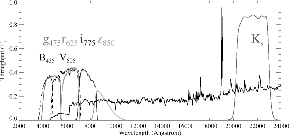
Figure 1.— Total effective throughput of the HST/ACS $g_{475}$$r_{625}$$i_{775}$$z_{850}$ and VLT/ISAAC $K_{S}$ filters. The galaxy spectrum shown is the $SB2$ template from Benítez (2000) redshifted to $z=4.1$, and applying the attenuation prescription of Madau et al. (1996). The GOODS $B_{435}$ and $V_{606}$ filters are indicated by dashed lines for comparison.

Figure 2.— The ACS field showing $g_{475}$ in blue, $r_{625}$ in green and $z_{850}$ in red. The field measures 11.7 arcmin². The radio galaxy TN1338 stands out clearly as the bright green object (white circle).

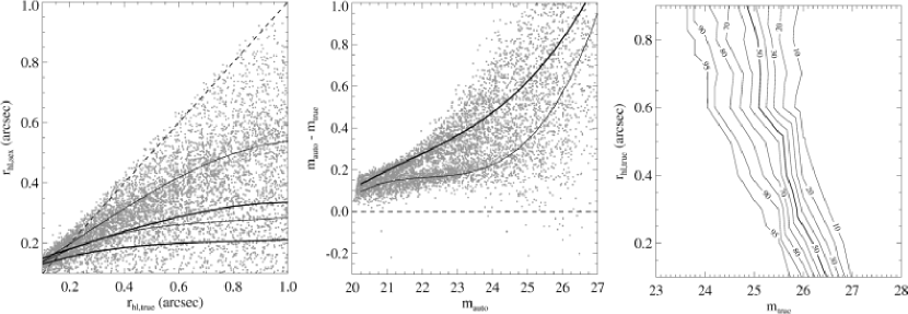
Figure 3.— Left: Intrinsic $r_{hl,z}$ versus $r_{hl,z}$ measured by SExtractor for de Vaucouleurs profiles (thick lines) and exponentials (thin lines). The difference between intrinsic and measured radius is smaller for exponentials. The intrinsic sizes are increasingly underestimated when going to fainter magnitudes, e.g. from $z_{850}$$\sim 24$ mag (top lines) to $z_{850}$$\sim 26$ mag (bottom lines). – Middle: The difference in $z_{850}$ between MAG_AUTO and total ‘intrinsic’ magnitudes for de Vaucouleurs profiles (thick line) and exponentials (thin line). Right: Completeness limits in $z_{850}$ as a function of total ‘intrinsic’ magnitudes and $r_{hl}$, where completeness is defined as the ratio of the number of objects detected to the number of artificial objects added to the image (50% exponential; 50% de Vaucouleurs). The 50% completeness limit lies at an intrinsic magnitude of $\approx 26.5$ for small sources. When expressed in terms of MAG_AUTO, the completeness limits shown here should be some $\sim$0.5–1.0 mag fainter, due to an underestimate of the ‘total’ flux for faint galaxies.

Figure 4.— $g_{475}$–$r_{625}$ versus $r_{625}$–$z_{850}$ for model simulations using the Bruzual & Charlot (2003) libraries. Grey points indicate the modeled colors of a large set of SEDs in the redshift range $0<z<6$ (see text for details). Galaxies at $z=4.1$ with ages less than 500 Myr are shown as large solid circles. Our selection criteria for selecting $g_{475}$-dropouts at $z\approx 4.1$ as defined by $g_{475}$–$r_{625}$$\geq 1.5$, $g_{475}$–$r_{625}$$\geq$$r_{625}$–$z_{850}$$+1.1$, $r_{625}$–$z_{850}$$\leq 1.0$ are indicated by the shaded area. The spectral tracks are an elliptical (red solid line), an Sbc (red dashed line), an Scd (red dotted line), and a 100 Myr constant star formation model with $E(B-V)=0.0$ mag (blue solid line) and $E(B-V)=0.2$ mag (blue dotted line). Redshifts are indicated along the tracks. The redshift of the overdensity of Venemans et al. (2002) is marked by the large blue squares ($z\approx 4.1$). Stars (green) mark the stellar locus based on the stellar library of Pickles (1998).

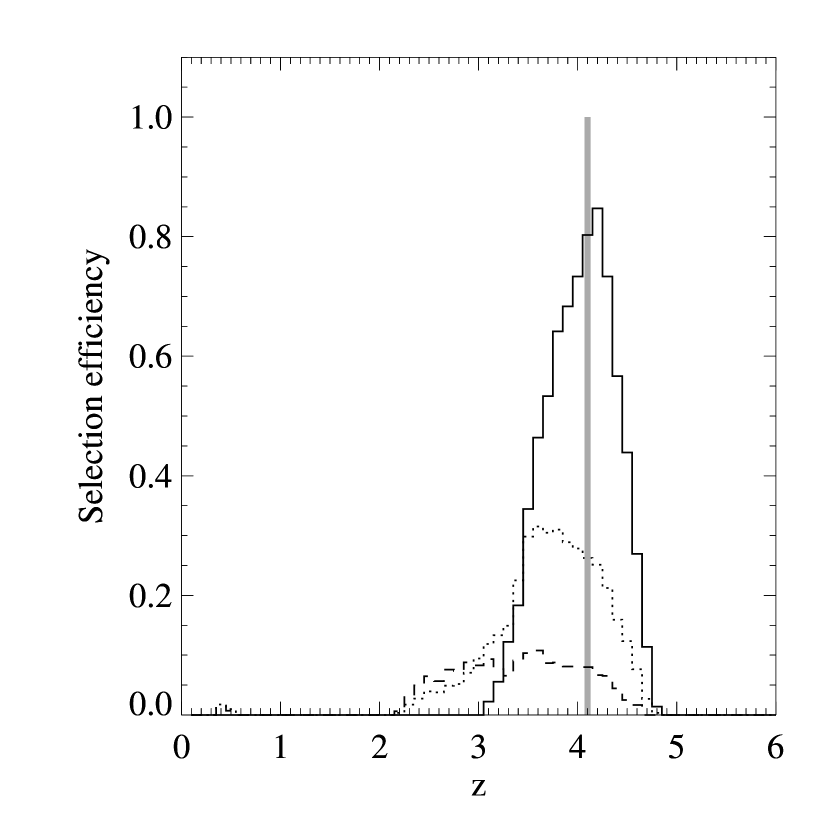
Figure 5.— Selection efficiency for $z\sim 4$ LBGs. The dotted histogram shows the fraction of model galaxies that meets the selection criteria in each redshift bin. The solid histogram shows the selection efficiency for model galaxies with ages less than 100 Myr and $0<E(B-V)<0.3$. The dashed histogram shows the fraction of models with ages greater than 0.5 Gyr selected, illustrating possible contamination of our $z\sim 4.1$ sample by relatively old galaxies at $z\sim 2.5$. A (minor) source of contamination is the possible inclusion of Balmer-break objects at $z\sim 0.5$. The shaded region indicates the redshift interval ($z=4.07-4.13$) of the protocluster defined by the radio galaxy and the Ly$\alpha$ emitters from Venemans et al. (2002).

Figure 6.— Colors and $g_{475}$-dropout samples derived from two different simulations of the TN1338 $g_{475}$$r_{625}$$i_{775}$$z_{850}$ data set. In the first simulation (left panel), the input model was transformed directly in terms of the TN1338 $g_{475}$$r_{625}$$i_{775}$$z_{850}$filter set. In the second (right panel), the model was first transformed in the terms of the GOODS $B_{435}$$V_{606}$$i_{775}$$z_{850}$filter set and then transformed to the TN1338 $g_{475}$$r_{625}$$i_{775}$$z_{850}$ filter set using the transformation method laid out in Section 2.7. Objects detected in the images are indicated by small circles. Objects falling within our $g_{475}$-dropout selection window (marked by thick lines) are indicated by the large squares. Note that the transformation from model to GOODS to TN1338 (right panel) introduces some small changes in the color distributions with respect to the transformation directly from model to TN1338 (left panel). This is due to the fact that in the right panel object detection and color selection are performed twice, and because of uncertainties introduced by determining the photometric redshifts of the objects in the simulated GOODS images. However, the $g_{475}$-dropout selections obtained from the images generated from our transformation method are nearly identical in number to those obtained from direct simulations of the same data set. This suggests that it is reasonable to use the $g_{475}$-dropout samples obtained from the transformed images for quantifying the expected number densities (see Section 5).

Figure 7.— Color-color diagram of $g_{475}$-dropouts in TN1338 (large circles) and the detection catalog (grey points). The shaded region shows our selection window (Eq. 1). Confirmed LAEs from Venemans et al. (2002) are marked by red stars, and the radio galaxy by the large black square. Small green stars mark the stellar locus based on the stellar SED library of Pickles (1998). See the caption of Fig. 4 for further details.

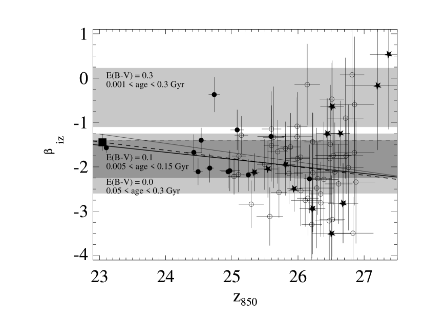
Figure 8.— $z_{850}$ versus $\beta_{iz}$ for $g_{475}$-dropouts detected/undetected in $K_{S}$ (filled/open circles), LAEs (stars), and the radio galaxy (square). The best-fit linear relations are indicated (thick lines, see text for details). The thin solid line is the relation for $B_{435}$-dropouts (R.J. Bouwens, private communication). The best-fit SED from Papovich et al. (2001) redshifted to $z=4$ has $\beta_{iz}\approx-1.4$ (thin dashed line). Shaded regions are for $E(B-V)=0.0$ mag with ages between 0.05 and 0.3 Gyr (bottom light shaded region), $E(B-V)=0.1$ mag with ages between 0.005 and 0.15 Gyr (dark shaded region), and $E(B-V)=0.3$ mag with ages between 0.001 and 0.3 Gyr (top light shaded region), assuming an exponential star formation history ($\tau=10$ Myr) with $0.2Z_{\odot}$ metallicity and a Salpeter IMF.

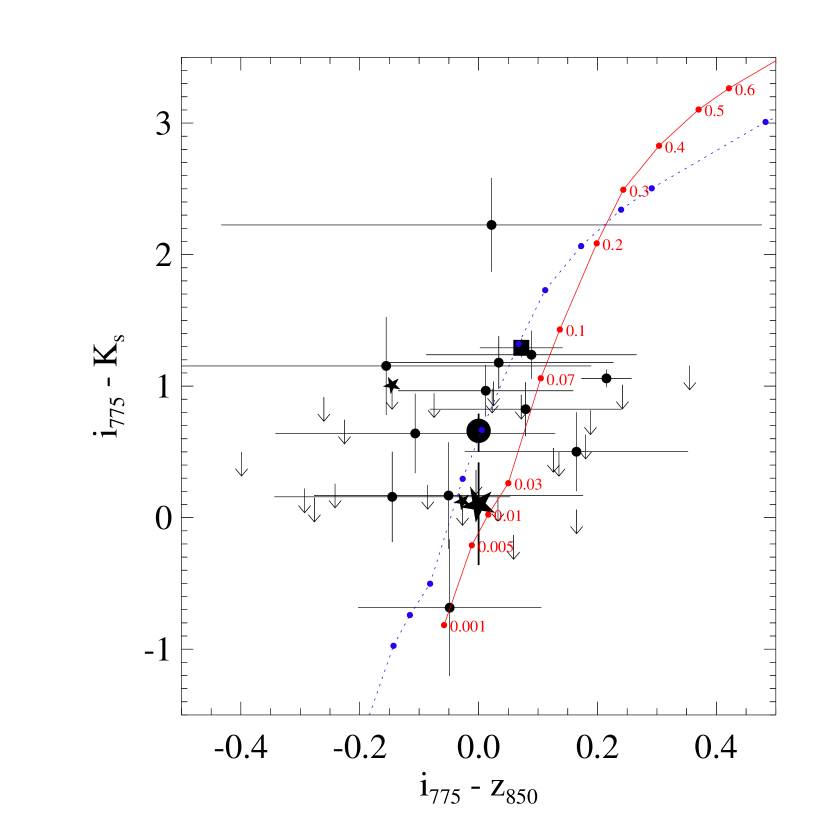
Figure 9.— Rest-frame UV-optical colors of the $g_{475}$-dropouts (circles), the LAEs L9 and L25 (stars), and the radio galaxy (square). Arrows indicate $2\sigma$ limits for non-detections in $K_{S}$ (errors omitted for clarity). Lines indicate the colors of a $\tau=10$ Myr SED ($0.2Z_{\odot}$) with ages in Gyr along the track for $E(B-V)=0.0$ mag (dotted) and $E(B-V)=0.15$ mag (solid). The large circle was obtained from a $K_{S}$-band stack of 12 $g_{475}$-dropouts having 25.3$<$$i_{775}$$<$26.4 mag. The large star was obtained from a $K_{S}$-band stack of 5 LAEs within a similar magnitude range. Their $i_{775}$–$K_{S}$ colors differ by $\sim 0.7$ mag.

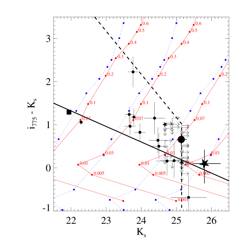
Figure 10.— Color-magnitude diagram of the $g_{475}$-dropouts (circles). The dashed line indicates the approximate $2\sigma$ detection limits. The tracks are for $\tau=10$ Myr SEDs with different stellar masses of 0.03, 0.1, 0.5 and 2$\times 10^{10}$ M_⊙ for $E(B-V)=0.0$ mag (dotted) and $E(B-V)=0.15$ mag (solid). The thick solid line indicates the ‘blue envelope’ of Papovich et al. (2004), and suggests a color-magnitude relation in which luminosity correlates with either age or dust. See the caption of Fig. 9 for further details.

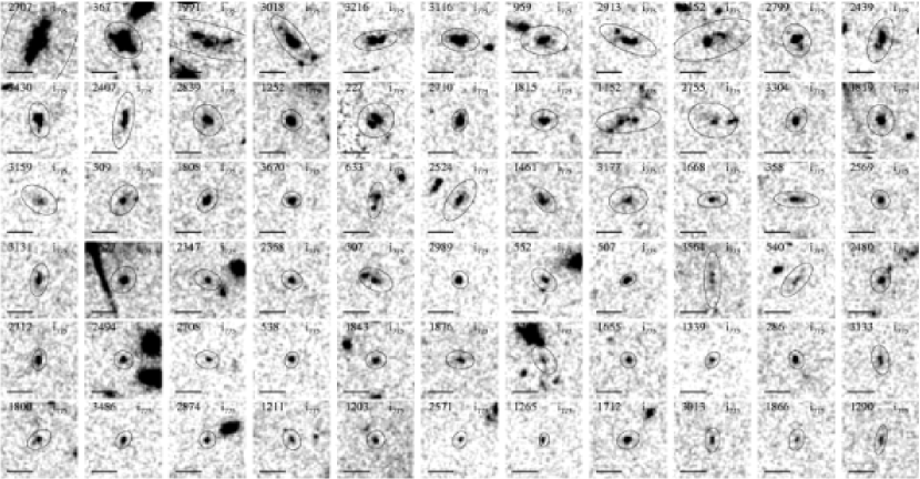
Figure 11.— $i_{775}$ postage stamps ($3\arcsec\times 3\arcsec$) of the $g_{475}$-dropout sample. The images have been smoothed using a Gaussian kernel of 0$\farcs$075 (FWHM). Kron apertures are indicated. The scale bars measure 1″. North is up, East is to the left.

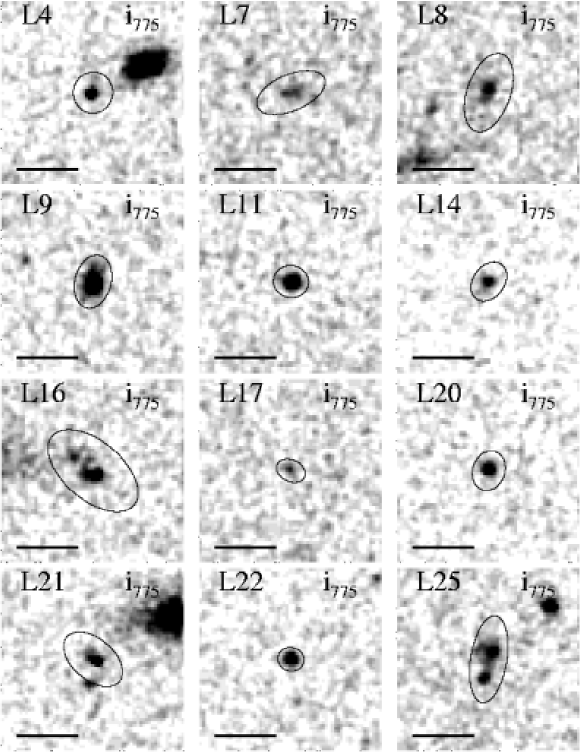
Figure 12.— $i_{775}$ postage stamps ($3\arcsec\times 3\arcsec$) of the twelve spectroscopically confirmed Ly$\alpha$ emitters of Venemans et al. (2002). See the caption of Fig. 11 for details.

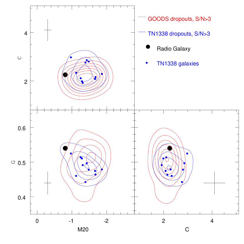
Figure 13.— The morphological Gini coefficient ($G$), $M_{20}$, and concentration ($C$) for the $g_{475}$-dropouts in TN1338 (blue points and contours). The parameter distributions determined from $\sim$70 LBGs at $z\sim 4$ selected in the GOODS CDF-S field are shown for comparison (red contours). The radio galaxy is indicated by the large black circle. The approximate size of the error bars on the measurements are indicated in a corner of each panel.

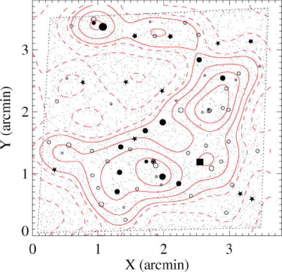
Figure 14.— Object map of the $g_{475}$-dropout candidates (circles), TN J1338–1942 (square), Ly$\alpha$ emitters (stars) and the detection catalog (points). $g_{475}$-dropouts detected in $K_{S}$ are indicated by filled circles. Larger circles indicate brighter objects in $z_{850}$. The contours represent density fluctuations $\Delta\equiv(\Sigma-\bar{\Sigma})/\bar{\Sigma}$ of –1, –0.5, –0.1 (dashed contours) and +0.1, +0.5, +1, +1.5 (solid contours), achieved by smoothing the object map with a Gaussian of width 36″, or 250 kpc (FWHM), using equal weights. LAEs that are not in the $g_{475}$-dropout sample were not included in the density contours.

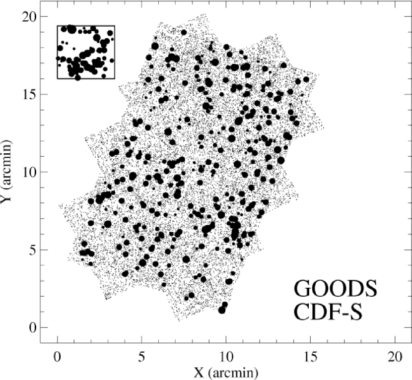
Figure 15.— Distribution of $z\sim 4$ LBGs in the CDF-S GOODS field with $z_{850}$$\leq 27.0$ mag (circles). Larger symbols correspond to brighter objects. The inset in the top left shows the $3\farcm 4\times 3\farcm 4$ TN1338 field and the distribution of $g_{475}$-dropouts at the same scale as the CDF-S GOODS field for comparison.

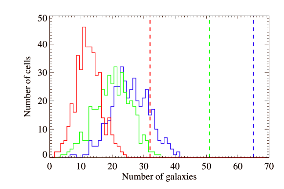
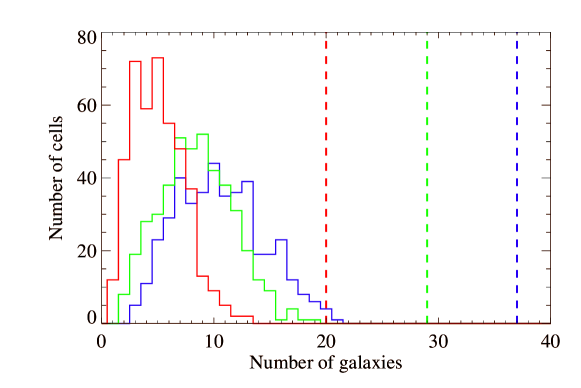
Figure 16.— Counts in cells analysis of $z\sim 4$ LBGs in the GOODS simulations compared to TN1338. Top panel: Histograms of the number of objects in square cells the size of TN1338 ($3\farcm 4\times 3\farcm 4$) for $z_{850}$$<$27.0 (blue), 26.5 (green) and 26.0 mag (red). The number of $g_{475}$-dropouts in TN1338 are indicated by the vertical lines of corresponding color. Bottom panel: Same as top, but for $2\farcm 1\times 2\farcm 1$ cells. The number of $g_{475}$-dropouts in TN1338 exceeds the number encountered in GOODS for each limiting magnitude and cell size.

Figure 17.— The angular two-point correlation function for $g_{475}$-dropouts in the TN1338 field (solid points). The solid line indicates the angular correlation function $w(\theta)=0.6\theta^{-0.6}$, as measured for $B_{435}$-dropouts with $z_{850}$$\lesssim 26.5$ mag in GOODS (Lee et al., 2006). The shaded region indicates the $1\sigma$ spread in $w(\theta)$ at each $\theta$ that was measured among 25 $3\farcm 4\times 3\farcm 4$ fields of the same geometry and source density as the TN1338 field extracted from a $17\arcmin\times 17\arcmin$ mock catalog with $w(\theta)\approx 0.6\theta^{-0.6}$.

Figure 18.— Total $z_{B}$ probability distributions for $g_{475}$-dropouts in TN1338 (blue) and in the CDF-S GOODS field (red). The area under the blue curve is equal to the number of objects in the TN1338 sample. The red curve for GOODS has been normalised to the area of the TN1338 field. The GOODS curve was subtracted from the TN1338 curve to bring out the residuals of the redshift distribution for TN1338 (black curve). The residual peaks at the redshift of the radio galaxy and LAEs (shaded region). A secondary peak of 1 object lies at $z_{B}\approx 3.8$, the redshift of the other $\sim 6L^{*}$ object in the field. The peaks at $z\sim 0.5$ are due to the alternative probability that a fraction of the $g_{475}$-dropouts could be 4000Å break objects.

Figure 19.— VLT/FORS2 spectrum of object #367 with a redshift of $3.830\pm 0.002$.

References

- Adelberger et al. (1998) Adelberger, K. L., Steidel, C. C., Giavalisco, M., Dickinson, M., Pettini, M., & Kellogg, M. 1998, ApJ, 505, 18
- Beckwith et al. (2006) Beckwith, S. V. W., et al. 2006, AJ, 132, 1729
- Benítez (2000) Benítez, N. 2000, ApJ, 536, 571
- Benítez et al. (2004) Benítez, N. et al. 2004, ApJS, 150, 1
- Bertin & Arnouts (1996) Bertin, E., & Arnouts, S. 1996, A&AS, 117, 393
- Best et al. (2003) Best, P. N., Lehnert, M. D., Miley, G. K., & Röttgering, H. J. A. 2003, MNRAS, 343, 1
- Blakeslee et al. (2003) Blakeslee, J. P., Anderson, K. R., Meurer, G. R., Benítez, N., & Magee, D. 2003a, in ASP Conf. Ser. 295: Astronomical Data Analysis Software and Systems XII, 257
- Blakeslee et al. (2003) Blakeslee, J. P., et al. 2003, ApJ, 596, L143
- Blakeslee et al. (2006) Blakeslee, J. P., et al. 2006, ApJ, 644, 30
- Bouwens et al. (2003a) Bouwens, R., Broadhurst, T., & Illingworth, G. 2003a, ApJ, 593, 640
- Bouwens et al. (2004a) Bouwens, R. J., Illingworth, G. D., Blakeslee, J. P., Broadhurst, T. J., & Franx, M. 2004a, ApJ, 611, L1
- Bouwens et al. (2004b) Bouwens, R. J. et al. 2004b, ApJ, 606, L25
- Bouwens et al. (2004c) Bouwens, R. J. et al. 2004c, ApJ, 616, L79
- Bouwens & Illingworth (2006) Bouwens, R. J., & Illingworth, G. D. 2006, Nature, 443, 189
- Bouwens et al. (2006) Bouwens, R. J., Illingworth, G. D., Blakeslee, J. P., & Franx, M. 2006, ApJ, 653, 53
- Bouwens et al. (2007) Bouwens, R. J., Illingworth, G. D., Franx, M., & Ford, H. 2007, ApJ, in press (astro-ph/arXiv:0707.2080)
- Brocklehurst (1971) Brocklehurst, M. 1971, MNRAS, 153, 471
- Bruzual & Charlot (2003) Bruzual, G., & Charlot, S. 2003, MNRAS, 344, 1000
- Bruzual (2007) Bruzual, A. G. 2007, IAU Symposium, 241, 125
- Calzetti et al. (2000) Calzetti, D., Armus, L., Bohlin, R. C., Kinney, A. L., Koornneef, J., & Storchi-Bergmann, T. 2000, ApJ, 533, 682
- Charlot & Fall (1993) Charlot, S., & Fall, S. M. 1993, ApJ, 415, 580
- Coe et al. (2006) Coe, D., Benítez, N., Sánchez, S. F., Jee, M., Bouwens, R., & Ford, H. 2006, AJ, 132, 926
- Coleman et al. (1980) Coleman, G. D., Wu, C.-C., & Weedman, D. W. 1980, ApJS, 43, 393
- Conselice (2003) Conselice, C. J. 2003, ApJS, 147, 1
- Croft et al. (2005) Croft, S., Kurk, J., van Breugel, W., Stanford, S. A., de Vries, W., Pentericci, L., & Röttgering, H. 2005, AJ, 130, 867
- Daddi et al. (2002) Daddi, E. et al. 2002, A&A, 384, L1
- De Breuck et al. (2002) De Breuck, C., van Breugel, W., Stanford, S. A., Röttgering, H., Miley, G., & Stern, D. 2002, AJ, 123, 637
- De Lucia et al. (2004) De Lucia, G., Kauffmann, G., Springel, V., White, S. D. M., Lanzoni, B., Stoehr, F., Tormen, G., & Yoshida, N. 2004, MNRAS, 348, 333
- De Lucia et al. (2006) De Lucia, G., Springel, V., White, S. D. M., Croton, D., & Kauffmann, G. 2006, MNRAS, 366, 499
- Dey et al. (1997) Dey, A., van Breugel, W., Vacca, W. D., & Antonucci, R. 1997, ApJ, 490, 698
- Dressler et al. (1999) Dressler, A., Smail, I., Poggianti, B. M., Butcher, H., Couch, W. J., Ellis, R. S., & Oemler, A. J. 1999, ApJS, 122, 51
- Elston et al. (1988) Elston, R., Rieke, G. H., & Rieke, M. J. 1988, ApJ, 331, L77
- Eminian et al. (2007) Eminian, C., Kauffmann, G., Charlot, S., Wild, V., Bruzual, G., Rettura, A., & Loveday, J. 2007, MNRAS, submitted (arXiv:0709.1147)
- Ettori (2005) Ettori, S. 2005, MNRAS, 362, 110
- Ferguson et al. (2004) Ferguson, H. C. et al. 2004, ApJ, 600, L107
- Ford et al. (1998) Ford, H. C. et al. 1998, in Proc. SPIE Vol. 3356, p. 234-248, Space Telescopes and Instruments V, Pierre Y. Bely; James B. Breckinridge; Eds., 234–248
- Francis et al. (2001) Francis, P. J. et al. 2001, ApJ, 554, 1001
- Franx et al. (2003) Franx, M. et al. 2003, ApJ, 587, L79
- Gawiser et al. (2006) Gawiser, E., et al. 2006, ApJ, 642, L13
- Giavalisco et al. (1998) Giavalisco, M., Steidel, C. C., Adelberger, K. L., Dickinson, M. E., Pettini, M., & Kellogg, M. 1998, ApJ, 503, 543
- Giavalisco & Dickinson (2001) Giavalisco, M., & Dickinson, M. 2001, ApJ, 550, 177
- Giavalisco et al. (2004a) Giavalisco, M. et al. 2004a, ApJ, 600, L103
- Giavalisco et al. (2004b) Giavalisco, M. et al. 2004b, ApJ, 600, L93
- Glazebrook et al. (2004) Glazebrook, K., et al. 2004, Nature, 430, 181
- Goto et al. (2005) Goto, T. et al. 2005, ApJ, 621, 188
- Hall et al. (2001) Hall, P. B. et al. 2001, AJ, 121, 1840
- Holden et al. (2005) Holden, B. P. et al. 2005, ApJ, 620, L83
- Homeier et al. (2006) Homeier, N. L., et al. 2006, ApJ, 647, 256
- Intema et al. (2006) Intema, H. T., Venemans, B. P., Kurk, J. D., Ouchi, M., Kodama, T., Röttgering, H. J. A., Miley, G. K., & Overzier, R. A. 2006, A&A, 456, 433
- Kaiser (1984) Kaiser, N. 1984, ApJ, 284, L9
- Kajisawa et al. (2006) Kajisawa, M., Kodama, T., Tanaka, I., Yamada, T., & Bower, R. 2006, MNRAS, 371, 577
- Kashikawa et al. (2006) Kashikawa, N., et al. 2006, ApJ, 637, 631
- Kashikawa et al. (2007) Kashikawa, N., Kitayama, T., Doi, M., Misawa, T., Komiyama, Y., & Ota, K. 2007, ApJ, 663, 765
- Kauffmann et al. (2004) Kauffmann, G., White, S. D. M., Heckman, T. M., Ménard, B., Brinchmann, J., Charlot, S., Tremonti, C., & Brinkmann, J. 2004, MNRAS, 353, 713
- Keel et al. (1999) Keel, W. C., Cohen, S. H., Windhorst, R. A., & Waddington, I. 1999, AJ, 118, 2547
- Kennicutt (1998) Kennicutt, R. C. 1998, ApJ, 498, 541
- Kinney et al. (1996) Kinney, A. L., Calzetti, D., Bohlin, R. C., McQuade, K., Storchi-Bergmann, T., & Schmitt, H. R. 1996, ApJ, 467, 38
- Kodama et al. (2007) Kodama, T., Tanaka, I., Kajisawa, M., Kurk, J., Venemans, B., De Breuck, C., Vernet, J., & Lidman, C. 2007, MNRAS, 377, 1717
- Kravtsov et al. (2004) Kravtsov, A. V., Berlind, A. A., Wechsler, R. H., Klypin, A. A., Gottlöber, S., Allgood, B., & Primack, J. R. 2004, ApJ, 609, 35
- Kron (1980) Kron, R. G. 1980, ApJS, 43, 305
- Kunth et al. (2003) Kunth, D., Leitherer, C., Mas-Hesse, J. M., Östlin, G., & Petrosian, A. 2003, ApJ, 597, 263
- Kurk et al. (2003) Kurk, J., Röttgering, H., Pentericci, L., Miley, G., & Overzier, R. 2003, New Astronomy Review, 47, 339
- Landy & Szalay (1993) Landy, S. D., & Szalay, A. S. 1993, ApJ, 412, 64
- Lee et al. (2006) Lee, K.-S., Giavalisco, M., Gnedin, O. Y., Somerville, R. S., Ferguson, H. C., Dickinson, M., & Ouchi, M. 2006, ApJ, 642, 63
- Li et al. (2006) Li, Y., Hernquist, L., Robertson, B., Cox, T.J., Hopkins, P.F., Springel, V., Gao, L., Di Matteo, T., Zentner, A.R., Jenkins, A., & Yoshida, N. 2007, ApJ, 665, 187
- Ling et al. (1986) Ling, E. N., Barrow, J. D., & Frenk, C. S. 1986, MNRAS, 223, 21P
- Lotz et al. (2004) Lotz, J. M., Primack, J., & Madau, P. 2004, AJ, 128, 163
- Lotz et al. (2006) Lotz, J. M., Madau, P., Giavalisco, M., Primack, J., & Ferguson, H. C. 2006, ApJ, 636, 592
- Madau (1995) Madau, P. 1995, ApJ, 441, 18
- Madau et al. (1996) Madau, P., Ferguson, H. C., Dickinson, M. E., Giavalisco, M., Steidel, C. C., & Fruchter, A. 1996, MNRAS, 283, 1388
- Madau et al. (1998) Madau, P., Pozzetti, L., & Dickinson, M. 1998, ApJ, 498, 106
- Maraston et al. (2006) Maraston, C., Daddi, E., Renzini, A., Cimatti, A., Dickinson, M., Papovich, C., Pasquali, A., & Pirzkal, N. 2006, ApJ, 652, 85
- McCarthy et al. (2001) McCarthy, P. J. et al. 2001, ApJ, 560, L131
- Mei et al. (2006) Mei, S., et al. 2006, ApJ, 644, 759
- Meurer et al. (1999) Meurer, G. R., Heckman, T. M., & Calzetti, D. 1999, ApJ, 521, 64
- Miley et al. (2004) Miley, G. K. et al. 2004, Nature, 427, 47
- Miley et al. (2006) Miley, G. K., et al. 2006, ApJ, 650, L29
- Mo et al. (1998) Mo, H. J., Mao, S., & White, S. D. M. 1998, MNRAS, 295, 319
- Mo & White (2002) Mo, H. J., & White, S. D. M. 2002, MNRAS, 336, 112
- Möller & Fynbo (2001) Möller, P., & Fynbo, J. U. 2001, A&A, 372, L57
- Mullis et al. (2005) Mullis, C. R., Rosati, P., Lamer, G., Böhringer, H., Schwope, A., Schuecker, P., & Fassbender, R. 2005, ApJ, 623, L85
- Nilsson et al. (2007) Nilsson, K. K., et al. 2007, A&A, 471, 71
- Oke (1971) Oke, J. B. 1971, ApJ, 170, 193
- Ouchi et al. (2004a) Ouchi, M., et al. 2004a, ApJ, 611, 660
- Ouchi et al. (2004b) Ouchi, M., et al. 2004b, ApJ, 611, 685
- Ouchi et al. (2005a) Ouchi, M., et al. 2005a, ApJ, 635, L117
- Ouchi et al. (2005b) Ouchi, M., et al. 2005b, ApJ, 620, L1
- Ouchi et al. (2007) Ouchi, M., et al. 2007, ApJ, submitted (astro-ph/arXiv:0707.3161)
- Overzier et al. (2006a) Overzier, R. et al. 2006a, ApJ, 637, 1
- Overzier (2006b) Overzier, R. A. 2006b, Ph.D. Thesis, Universiteit Leiden
- Papovich et al. (2001) Papovich, C., Dickinson, M., & Ferguson, H. C. 2001, ApJ, 559, 620
- Papovich et al. (2004) Papovich, C. et al. 2004, ApJ, 600, L111
- Pascarelle et al. (1996) Pascarelle, S. M., Windhorst, R. A., Driver, S. P., Ostrander, E. J., & Keel, W. C. 1996, ApJ, 456, L21
- Pentericci et al. (2000) Pentericci, L. et al. 2000, A&A, 361, L25
- Pentericci et al. (2001) Pentericci, L., McCarthy, P. J., Röttgering, H. J. A., Miley, G. K., van Breugel, W. J. M., & Fosbury, R. 2001, ApJS, 135, 63
- Pentericci et al. (2002) Pentericci, L., Kurk, J. D., Carilli, C. L., Harris, D. E., Miley, G. K., & Röttgering, H. J. A. 2002, A&A, 396, 109
- Pentericci et al. (2007) Pentericci, L., Grazian, A., Fontana, A., Salimbeni, S., Santini, P., De Santis, C., Gallozzi, S., & Giallongo, E. 2007, A&A, 471, 433
- Peter et al. (2007) Peter, A. H. G., Shapley, A. E., Law, D. R., Steidel, C. C., Erb, D. K., Reddy, N. A., & Pettini, M. 2007, ApJ, in press (arXiv:astro-ph/0706.2865)
- Petrosian (1976) Petrosian, V. 1976, ApJ, 209, L1
- Pickles (1998) Pickles, A. J. 1998, PASP, 110, 863
- Pirzkal et al. (2006) Pirzkal, N., Malhotra, S., Rhoads, J. E., & Xu, C. 2007, ApJ, 667, 49
- Porciani & Giavalisco (2002) Porciani, C., & Giavalisco, M. 2002, ApJ, 565, 24
- Postman et al. (2005) Postman, M., et al. 2005, ApJ, 623, 721
- Quadri et al. (2007) Quadri, R., et al. 2007, ApJ, 654, 138
- Rettura et al. (2006) Rettura, A., et al. 2006, A&A, 458, 717
- Salpeter (1955) Salpeter, E. E. 1955, ApJ, 121, 161
- Sánchez & González-Serrano (1999) Sánchez, S. F., & González-Serrano, J. I. 1999, A&A, 352, 383
- Sánchez & González-Serrano (2002) Sánchez, S. F., & González-Serrano, J. I. 2002, A&A, 396, 773
- Schlegel et al. (1998) Schlegel, D. J., Finkbeiner, D. P., & Davis, M. 1998, ApJ, 500, 525
- Seymour et al. (2007) Seymour, N., et al. 2007, ApJS, 171, 353
- Shapley et al. (2003) Shapley, A. E., Steidel, C. C., Pettini, M., & Adelberger, K. L. 2003, ApJ, 588, 65
- Sheth & Tormen (1999) Sheth, R. K., & Tormen, G. 1999, MNRAS, 308, 119
- Shimasaku et al. (2003) Shimasaku, K. et al. 2003, ApJ, 586, L111
- Sirianni et al. (2005) Sirianni, M., et al. 2005, PASP, 117, 1049
- Somerville et al. (2004) Somerville, R. S., Lee, K., Ferguson, H. C., Gardner, J. P., Moustakas, L. A., & Giavalisco, M. 2004, ApJ, 600, L171
- Soneira & Peebles (1978) Soneira, R. M., & Peebles, P. J. E. 1978, AJ, 83, 845
- Spergel et al. (2003) Spergel, D. N. et al. 2003, ApJS, 148, 175
- Springel et al. (2005) Springel, V. et al. 2005, Nature, 435, 629
- Stanford et al. (1998) Stanford, S. A., Eisenhardt, P. R., & Dickinson, M. 1998, ApJ, 492, 461
- Stanford et al. (2006) Stanford, S. A., et al. 2006, ApJ, 646, L13
- Steidel et al. (1998) Steidel, C. C., Adelberger, K. L., Dickinson, M., Giavalisco, M., Pettini, M., & Kellogg, M. 1998, ApJ, 492, 428
- Steidel et al. (1999) Steidel, C. C., Adelberger, K. L., Giavalisco, M., Dickinson, M., & Pettini, M. 1999, ApJ, 519, 1
- Steidel et al. (2000) Steidel, C. C., Adelberger, K. L., Shapley, A. E., Pettini, M., Dickinson, M., & Giavalisco, M. 2000, ApJ, 532, 170
- Steidel et al. (2005) Steidel, C. C., Adelberger, K. L., Shapley, A. E., Erb, D. K., Reddy, N. A., & Pettini, M. 2005, ApJ, 626, 44
- Stiavelli et al. (2005) Stiavelli, M. et al. 2005, ApJ, 622, L1
- Suwa et al. (2006) Suwa, T., Habe, A., & Yoshikawa, K. 2006, ApJ, 646, L5
- Szalay et al. (1999) Szalay, A. S., Connolly, A. J., & Szokoly, G. P. 1999, AJ, 117, 68
- Thompson et al. (2000) Thompson, D., Aftreth, O., & Soifer, B. T. 2000, AJ, 120, 2331
- van Dokkum et al. (2003) van Dokkum, P. G. et al. 2003, ApJ, 587, L83
- van Dokkum et al. (2000) van Dokkum, P. G., Franx, M., Fabricant, D., Illingworth, G. D., & Kelson, D. D. 2000, ApJ, 541, 95
- Venemans et al. (2002) Venemans, B. P. et al. 2002, ApJ, 569, L11
- Venemans et al. (2004) Venemans, B. P. et al. 2004, A&A, 424, L17
- Venemans et al. (2005) Venemans, B. P. et al. 2005, A&A, 431, 793
- Venemans et al. (2007) Venemans, B. P. et al. 2007, A&A, 461, 823
- Villar-Martín et al. (2005) Villar-Martín, M. et al. 2005, MNRAS, L112
- Wang et al. (2004) Wang, J. X. et al. 2004, ApJ, 608, L21
- Webb et al. (2006) Webb, T. M. A., et al. 2006, ApJ, 636, L17
- Wold et al. (2003) Wold, M., Armus, L., Neugebauer, G., Jarrett, T. H., & Lehnert, M. D. 2003, AJ, 126, 1776
- Wuyts et al. (2004) Wuyts, S., van Dokkum, P. G., Kelson, D. D., Franx, M., & Illingworth, G. D. 2004, ApJ, 605, 677
- Zheng et al. (2006) Zheng, W., et al. 2006, ApJ, 640, 574
- Zirm et al. (2005) Zirm, A. W. et al. 2005, ApJ, 630, 68