thanks: ANPCyT Fellowthanks: CONICET Fellowthanks: Member of Carrera del Investigador Científico (CONICET, Argentina)

Luminosity distance for Born-Infeld electromagnetic waves propagating in a cosmological magnetic background

Matías Aiello aiello@iafe.uba.ar Instituto de Astronomía y Física del Espacio, Casilla de Correo 67, Sucursal 28, 1428 Buenos Aires, Argentina Departamento de Física, Facultad de Ciencias Exactas y Naturales, Universidad de Buenos Aires, Ciudad Universitaria, Pabellón I, 1428 Buenos Aires, Argentina    Gabriel R. Bengochea gabriel@iafe.uba.ar Instituto de Astronomía y Física del Espacio, Casilla de Correo 67, Sucursal 28, 1428 Buenos Aires, Argentina Departamento de Física, Facultad de Ciencias Exactas y Naturales, Universidad de Buenos Aires, Ciudad Universitaria, Pabellón I, 1428 Buenos Aires, Argentina    Rafael Ferraro ferraro@iafe.uba.ar Instituto de Astronomía y Física del Espacio, Casilla de Correo 67, Sucursal 28, 1428 Buenos Aires, Argentina Departamento de Física, Facultad de Ciencias Exactas y Naturales, Universidad de Buenos Aires, Ciudad Universitaria, Pabellón I, 1428 Buenos Aires, Argentina
Abstract

Born-Infeld electromagnetic waves interacting with a static magnetic background are studied in an expanding universe. The non-linear character of Born-Infeld electrodynamics modifies the relation between the energy flux and the distance to the source, which gains a new dependence on the redshift that is governed by the background field. We compute the luminosity distance as a function of the redshift and compare with Maxwellian curves for supernovae type Ia.

Born-Infeld, waves, light propagation, cosmology, accelerated expansion
pacs:
Valid PACS appear here

I Introduction

The discovery of an unexpected diminution in the observed energy fluxes coming from supernovae type Ia Riess-Perlmutter , which are thought of as standard candles, has been interpreted in the context of the standard cosmological model as evidence for an accelerating universe dominated by something called dark energy. This fact is one of the most puzzling and deepest problems in cosmology and fundamental physics today. Although the cosmological constant seems to be the simplest explanation for the phenomenon, several dynamical scenarios have been tried out (see, for instance, padmanabhan and references therein). It is worthwhile to emphasize that the evidence for an accelerating universe mainly relies on energy flux measurements for type Ia supernovae at different values of cosmological redshifts. They provide the most direct and consistent way to determine the recent expansion history of the universe. Nevertheless the relation between the cosmological redshift and the energy flux for a point-like source involves not only the evolution of the universe during the light journey but some assumptions about the nature of the light itself. Customarily, one accepts the linear Maxwell theory to describe the light propagation, where light propagates without interacting with other electric or magnetic fields. However, in the context of non-linear electrodynamics the interaction between the light emitted from such distant sources and cosmological magnetic backgrounds modifies the relation between the redshift and the flux of energy. If this kind of effect were not correctly interpreted it could lead to an erroneous conclusion about the expansion history of the universe. Concretely, an effect coming from non-linear electrodynamics could explain the curves of luminosity distance vs redshift for type Ia supernovae without invoking dark energy. This remark drives us to study the propagation of non-linear electromagnetic waves in an expanding universe with a magnetic background. We will benefit from recently obtained results for Born-Infeld electromagnetic plane waves propagating in a magnetic uniform background in Minkowski space-time 9abf .

Born-Infeld electrodynamics 1born ; 2born is a non-linear theory for the electromagnetic field $F_{\mu\nu}$ governed by the Lagrangian

$${\cal L}=\sqrt{-g}\ \frac{b^{2}}{4\>\pi}\,\left(1-\sqrt{1+\frac{2S}{b^{2}}-\frac{P^{2}}{b^{4}}}\right)$$ (1)

where $b$ is a new fundamental constant and $S$ and $P$ are the scalar and pseudoscalar field invariants

$$S=\frac{1}{4}F_{\mu\nu}F^{\mu\nu}\ \ \ \ \ \ \ \ \ \ P=\frac{1}{4}\>^{*}F_{\mu\nu}F^{\mu\nu}$$ (2)

(in Minkowski space-time it is $2S=|{\bf{\mathbb{B}}}|^{2}-|{\bf{\mathbb{E}}}|^{2}$ and $P={\bf{\mathbb{E}}}\cdot{\bf{\mathbb{B}}}$, $\bf{\mathbb{E}}$ and $\bf{\mathbb{B}}$ being the electric and magnetic fields respectively). Born-Infeld electrodynamics goes to Maxwell electromagnetism when $b\rightarrow\infty$. In particular, the Born-Infeld field of a point-like charge reaches the finite value $b$ at the charge position and becomes Coulombian far from the charge. Born-Infeld theory is the only non-linear spin 1 field theory displaying causal propagation and absence of birefringence deser ; 5boi .

Nowadays, Born-Infeld theory is reborn in the context of superstrings because Born-Infeld-like Lagrangians emerge in the low energy limit of string theories strings . Born-Infeld-like Lagrangians have been also proposed to describe a matter dynamics able to drive the universe to an accelerated expansion varios . In spite of this revival of Born-Infeld’s ideas, there is no experimental evidence for Born-Infeld effects in electrodynamics: the value of $b$ remains unknown (see an upper bound for $b$ in Jack ).

In the next section we will summarize the recently obtained results on Born-Infeld waves propagating in Minkowski space-time in the presence of a uniform magnetic background 9abf . These results –properly adapted– will be used in section III to understand the Born-Infeld energy flux coming from a point-like source in a spatially flat Friedman-Robertson-Walker (FRW) expanding universe. In section IV we will reformulate the relation between the luminosity distance $d_{L}$ and the redshift $z$ within the framework of Born-Infeld electrodynamics. We will show that the presence of magnetic backgrounds modify the curves $d_{L}$ vs $z$, and we will analyze the consequences for the measurements of the luminosity distance of supernovae type Ia.

II Born-Infeld Plane waves in Minkowski space-time revisited

Free Born-Infeld electromagnetic plane waves do not differ from Maxwell plane waves. However, if the wave propagates in the presence of background fields then the propagation velocity becomes lower than $c$ as a consequence of the non-linearity of the theory. This issue has been studied in 5boi ; 3pleb ; 4pleb ; 6novello ; 7novello ; 8novello by considering the propagation of discontinuities. Recently the exact solution for a Born-Infeld electromagnetic plane wave propagating in a static uniform magnetic background has been obtained 9abf . The result retrieves the value for the phase velocity obtained in the above mentioned references:

$$\beta\ =\ \left(\frac{1+\frac{B_{L}^{2}}{b^{2}}}{1+\frac{B^{2}}{b^{2}}}\right)^{\frac{1}{2}}$$ (3)

where ${\bf B}=B_{L}\,\hat{x}+B_{B}\,\hat{y}+B_{E}\,\hat{z}$ is the background field and $B_{L}$ is its component along the propagation direction.

Furthermore, the results of 9abf exhibit an up to now unknown feature: the wave develops a longitudinal electric field which depends on $B_{L}$ and $B_{E}$ (the projection of the background field ${\bf B}$ on the polarization direction). In fact, the total electric and magnetic fields result

$\displaystyle{\bf{\mathbb{E}}}=\beta\ E_{wave}(\xi)\,\hat{z}+{\bf E}_{long}(\xi)\ ,$
$\displaystyle{\bf{\mathbb{B}}}=-E_{wave}(\xi)\,\hat{y}+{\bf B}$ (4)

where $E_{wave}(\xi)$ is the (usual) transversal electric field of the wave, and $\xi=x-\beta\,t$ is its phase. The longitudinal electric field of the wave is

$\displaystyle{\bf E}_{long}$ $\displaystyle=\frac{-{\bf B}\cdot\big{(}E_{wave}(\xi)\,\hat{z}\big{)}\ }{b^{2}\,\Big{(}1+\frac{B_{L}^{2}}{b^{2}}\Big{)}^{\frac{1}{2}}\Big{(}1+\frac{B^{2}}{b^{2}}\Big{)}^{\frac{1}{2}}}\ {\bf B}_{L}$ (5)
$\displaystyle=\frac{-B_{E}B_{L}\,E_{wave}(\xi)\ }{b^{2}\,\Big{(}1+\frac{B_{L}^{2}}{b^{2}}\Big{)}^{\frac{1}{2}}\Big{(}1+\frac{B^{2}}{b^{2}}\Big{)}^{\frac{1}{2}}}\ \hat{x}$

(of course ${\bf E}_{long}$ vanishes when $b\rightarrow\infty$). As a consequence, the Poynting vector ${\bf\cal S}$ acquires a component transverse to the propagation direction. In Born-Infeld electrodynamics the Poynting vector results

$${\bf\cal S}=\frac{1}{4\,\pi}\,\frac{{\bf{\mathbb{E}}}\times{\bf{\mathbb{B}}}}{\sqrt{1+b^{-2}\,(|{\bf{\mathbb{B}}}|^{2}-|{\bf{\mathbb{E}}}|^{2})-b^{-4}\,({\bf{\mathbb{E}}}\cdot{\bf{\mathbb{B}}})^{2}}}$$ (6)

For a wave $E_{wave}=E_{o}\cos(x-\beta t)$ the time averaged values of the transversal and longitudinal components of the Poynting vector associated with the field (4) are

$$<{\bf\cal S}_{\perp}>\ =\ \frac{E_{o}^{2}\,B_{L}\,{\bf B_{\perp}}}{8\,\pi\,b^{2}}\ +\ {\cal O}(b^{-4})$$ (7)
$$<{\cal S}_{x}>\ =\ \frac{E_{o}^{2}}{8\,\pi}\left[1\ -\ \frac{4B_{\perp}^{2}-2B_{E}^{2}+B_{L}^{2}}{2\,b^{2}}\right]\ +\ {\cal O}(b^{-4})$$ (8)

Notice that the transversal part of $<\boldsymbol{\cal S}>$ is parallel to the transversal background field ${\bf B_{\perp}}$. The angle $\alpha$ between the ray and the propagation direction is

$$\tan\alpha\ =\ \frac{B_{L}\ |{\bf B}_{\perp}|}{b^{2}}\ +\ {\cal O}(b^{-4})$$ (9)

Although this effect resembles the behavior of the extraordinary ray in anisotropic media, it should be emphasized that no birefringence exists in this case, which is a distinctive feature of Born-Infeld non-linear electrodynamics 5boi ; 6novello .

In Born-Infeld electrodynamics the energy density is

$$\rho=\frac{b^{2}}{4\ \pi}\left[\frac{1\ +\ b^{-2}\,|{\bf{\mathbb{B}}}|^{2}}{\sqrt{1+b^{-2}\,(|{\bf{\mathbb{B}}}|^{2}-|{\bf{\mathbb{E}}}|^{2})-b^{-4}\,({\bf{\mathbb{E}}}\cdot{\bf{\mathbb{B}}})^{2}}}-1\right]$$ (10)

Then, the time averaged energy density associated with the wave is

$\displaystyle<\rho>\ \ =$ $\displaystyle\frac{E_{o}^{2}}{8\pi}\bigg{[}1-\frac{3B_{\bot}^{2}-2B_{E}^{2}+B_{L}^{2}}{2\,b^{2}}\bigg{]}$ (11)
$\displaystyle+\frac{{B}^{2}}{8\,\pi}\bigg{[}1-\frac{{B}^{2}}{4b^{2}}\bigg{]}+\,{\cal O}(b^{-4})$

The above enumerated properties provides the rules to propagate Born-Infeld light rays in the presence of static uniform magnetic backgrounds.

III Born-Infeld Plane waves in an expanding flat FRW universe

In this section we will study the energy flux of Born-Infeld waves propagating in a spatially flat FRW expanding universe,

$$ds^{2}=a(\eta)^{2}(d\eta^{2}-dx^{2}-dy^{2}-dz^{2})$$ (12)

The conformal time $\eta$ is related with the cosmological time $t$ (the proper time of the comoving fluid) through the equation $dt=a(\eta)\,d\eta$. The energy-momentum conservation laws, $T^{\mu\nu}_{\ \ \ ;\nu}=0$, can be written as

$$\big{[}\sqrt{-g}\>T^{\mu\nu}\big{]}_{,\nu}+\Gamma^{\mu}_{\nu\rho}\>\sqrt{-g}\>T^{\rho\nu}=0$$ (13)

For the geometry (12) it is $\Gamma^{0}_{\nu\rho}=a_{,0}\,a^{-1}\,\delta_{\nu\rho}$, thus the energy balance becomes

$$a^{-2}\,\big{[}a^{4}\,T_{0}^{0}\big{]}_{,0}+a^{2}\,{T_{0}^{\alpha}}_{,\alpha}-a_{,0}\,a\ T=0$$ (14)

where $\alpha=1,2,3$ and $T=T_{\mu}^{\;\mu}$ is the trace of the energy-momentum tensor. We will use (14) to study electromagnetic waves propagating in a magnetic background; so, $T^{\nu}_{0}$ in (14) includes both the wave and the background fields. In Maxwell electromagnetism the trace $T$ is identically null. As a consequence, if $\{T_{0}^{\nu}\}^{M}$ solves (14) in Minkowski space-time ($a=constant$) then $\{T_{0}^{\nu}\}^{FRW}=a(\eta)^{-4}\,\{T_{0}^{\nu}\}^{M}$ will solve (14) in the spatially flat FRW universe. Since Maxwell energy-momentum tensor is quadratic in the fields, the former assertion means that the Maxwell fields scale with the factor $a(\eta)^{-2}$. This general conclusion is applicable to the particular case of a wave propagating in a magnetic background.

On the contrary, $T$ is non-null in Born-Infeld electrodynamics. Thus, the scaling of $T_{0}^{\nu}$ with the factor $a(\eta)^{-4}$ does not guarantee the fulfillment of (14). An additional correction is needed, which must vanish in the limit $b\rightarrow\infty$. We will search this correction to the lowest order in $b^{-2}$ for the Born-Infeld plane wave propagating in a magnetic background, whose main features were depicted in section II. Of course, we will assume that the magnetic background do not sensitively affects the homogeneity and isotropy of the space-time dominated by matter and (presumably) dark energy, because the energy density of the background field is negligible compared with matter and cosmological constant densities (a typical value for this field is $10^{-7}G$).

Since we are going to consider the lowest order correction in $b^{-2}$ for the magnitudes described in section II such as (5), (7), (8) and (11), we remark that any magnitude of this order or bigger will only require the Maxwellian scaling of the fields with the factor $a(\eta)^{-2}$. In the case of the propagation velocity (3) the correction can also be obtained from the results in 3pleb ; 6novello , where it is shown that the equation accomplished by the wave four-vector can be understood as if the rays propagate along null geodesics of an effective metric $\bar{g}_{\mu\nu}$. In the case of the Born-Infeld electrodynamics the effective metric $\bar{g}_{\mu\nu}$ is:

$$\bar{g}^{\mu\nu}=(b^{2}+\frac{1}{2}F_{\rho\sigma}F^{\rho\sigma})g^{\mu\nu}+F^{\mu}_{\ \lambda}F^{\lambda\nu}$$ (15)

where $g_{\mu\nu}$ is the space-time metric and $F_{\mu\nu}$ is the electromagnetic background where the ray propagates, in this case the components of the background are,

$$F_{xy}=-B_{E},\>\>F_{yz}=-B_{L},\>\>F_{xz}=B_{B}$$ (16)

For a ray propagating along the $x$ direction it is

$$d\bar{s}^{2}=\bar{g}_{\eta\eta}d\eta^{2}+\bar{g}_{xx}dx^{2}=0\Rightarrow\frac{dx}{d\eta}=\sqrt{-\frac{\bar{g}_{\eta\eta}}{\bar{g}_{xx}}}$$ (17)

When the effective metric (15) is evaluated for the magnetic background (16) it results

$$\bar{g}_{\eta\eta}=\frac{1}{\bigg{(}b^{2}+\frac{\textbf{B}^{2}}{a(\eta)^{4}}\bigg{)}a(\eta)^{2}}\>\>\>\>\>\>\>\>\>\>\>\>\>\bar{g}_{xx}=\frac{-1}{\bigg{(}b^{2}+\frac{B^{2}_{L}}{a(\eta)^{4}}\bigg{)}a(\eta)^{2}}$$ (18)

Thus, it is obtained

$$\beta(\eta)\ =\frac{dx}{d\eta}=\ \left(\frac{1+\frac{B_{L}^{2}}{a(\eta)^{4}b^{2}}}{1+\frac{B^{2}}{a(\eta)^{4}b^{2}}}\right)^{\frac{1}{2}}$$ (19)

By integrating the ray path in (17) we recognize that the phase $\xi$ has to be replaced with

$$\xi\ =\ x\ -\ \int^{\eta}\beta(\eta^{\prime})\ d\eta^{\prime}$$ (20)

(compare with the adiabatic treatment for an oscillator with slowly variable frequency goldstein ; birrel ). Notice that, since $\partial\xi/\partial x=1$ and $\partial\xi/\partial\eta=-\beta$ as in Minkowski space-time, then the derivatives of $T^{\mu}_{\nu}$ in (14) will preserve their Minkowskian structure. The trace of the Born-Infeld energy-momentum tensor is (see for instance 9abf )

$$T=\frac{b^{2}}{\pi}\left[\frac{1+b^{-2}\,S}{\sqrt{1+\frac{2S}{b^{2}}-\frac{P^{2}}{b^{4}}}}-1\right]=\frac{S^{2}+P^{2}}{2\pi\,b^{2}}+{\cal O}(b^{-4})$$ (21)

and scales with $a(\eta)^{-8}$. Let us consider a solution $\{T_{0}^{\nu}\}^{M}$ for the Born-Infeld field in Minkowski space-time; i.e., $\{T_{0}^{0}\}^{M}_{\ \ ,0}+\{T_{0}^{\alpha}\}^{M}_{\ \ ,\alpha}=0$ (for the case under consideration, $\{T_{0}^{0}\}^{M}$ is the energy density (11), and $\{T_{0}^{\alpha}\}^{M}$ are the components of the Poynting vector (7-8)). As stated above, the scaling of the fields with $a(\eta)^{-2}$ is not enough to get a solution for (14), since the term associated with the trace is now non-null. As the trace is of order $b^{-2}$, only $T_{0}^{\nu}$ has to be corrected in (14). So, let us try with the scaling $\{T_{0}^{\nu}\}^{FRW}=(1-\varepsilon\,a^{-4}\,b^{-2})\,a^{-4}\,\{T_{0}^{\nu}\}^{M}$. By replacing in (14) we obtain

$\displaystyle a^{-2}\,(1-\varepsilon\,a^{-4}\,b^{-2})(\{T_{0}^{0}\}^{M}_{\ \ ,0}+\{T_{0}^{\alpha}\}^{M}_{\ \ ,\alpha})$
$\displaystyle+4\,\varepsilon\,b^{-2}\,a_{,0}\,a^{-7}\,\{T_{0}^{0}\}^{M}-a_{,0}\,a^{-7}\ \{T\}^{M}=0$ (22)

Therefore

$$\varepsilon=b^{2}\frac{\{T\}^{M}}{4\,\{T_{0}^{0}\}^{M}}$$ (23)

Since the trace is of order $b^{-2}$, then $S$, $P$ and $\rho=T_{0}^{0}$ can be computed with the Maxwellian fields. The time averaged trace for a plane wave traveling in a magnetic background is 9abf

$$<\{T\}^{M}>\ =\ \frac{B^{4}+2E_{o}^{2}B_{\bot}^{2}}{8\pi b^{2}}$$ (24)

Thus $\varepsilon$ results

$$\varepsilon=\frac{B^{4}+2E_{o}^{2}B_{\bot}^{2}}{4(B^{2}+E_{o}^{2})}$$ (25)

IV Luminosity distance for a point-like source

According to the results of previous section, we should correct the Minkowskian Poynting vector (7), (8) with the factor $(1-\varepsilon\,a^{-4}\,b^{-2})\,a^{-4}$ pie1 . Thus the energy flux along the propagation direction is

$\displaystyle<{\cal S}_{x}>\ =\ \left(1-\frac{\varepsilon}{a(\eta)^{4}\,b^{2}}\right)\frac{E_{o}^{2}}{8\,\pi\,a(\eta)^{4}}$
$\displaystyle\left[1\ -\ \frac{4B_{\perp}^{2}-2B_{E}^{2}+B_{L}^{2}}{2\,a(\eta)^{4}b^{2}}\right]\ +\ {\cal O}(b^{-4})$
$\displaystyle=\ \left(1-\frac{\Delta_{B}}{a(\eta)^{4}\,b^{2}}\right)\frac{E_{o}^{2}}{8\,\pi\,a(\eta)^{4}}\ +\ {\cal O}(b^{-4})$ (26)

where $\Delta_{B}=2B_{\bot}^{2}-B_{E}^{2}+\frac{B_{L}^{2}}{2}+\frac{B^{4}+2E_{0}^{2}B_{\bot}^{2}}{4(B^{2}+E_{0}^{2})}$ is positive. Actually we are interested in light rays emitted from point-like sources in the universe. When a light ray travels in the intergalactic space, it undergoes a background magnetic field in different regions of the traveled path. In such case, the values of $B$, $B_{E}$, etc. implied in the propagation should be taken as representative values of the intergalactic background field along the ray trajectory; so $\Delta_{B}$ is a magnitude of the same order as the representative squared intergalactic field.

For a radial propagation the Minkowskian spherical energy flux is obtained from the plane flux by dividing by the square of the radial distance to the source $r^{2}=x^{2}+y^{2}+z^{2}$. Therefore the radial energy flux in a FRW spatially flat universe becomes

$$\mbox{\Fr F}\ =\ \left(1-\frac{\Delta_{B}}{a(\eta)^{4}\,b^{2}}\right)\frac{E_{o}^{2}}{8\,\pi\,a(\eta)^{4}\,r^{2}}\ +\ {\cal O}(b^{-4})$$ (27)

In Maxwell electrodynamics the background field does not interfere with the wave, but in non-linear Born-Infeld electrodynamics the first correction in (27) displays a coupling between the wave and the background magnetic field. The luminosity of an object results from integrating the flux at the time of emision $\eta_{e}$, this integration normalizes $E_{o}$ to fit the value of the luminosity $L$. By using (27) one obtains

$$L=\ \frac{E_{o}^{2}}{2\>a_{e}^{2}}\,\left(1-\frac{\Delta_{B}}{a_{e}^{4}\,b^{2}}\right)$$ (28)

Combining (27) and (28) the energy flux can be written as

$$\mbox{\Fr F}\ \simeq\ \frac{L\,a_{e}^{2}}{4\pi\>a(\eta)^{4}r^{2}}\left[1+\frac{\Delta_{B}}{a(\eta)^{4}\,b^{2}}\left(\frac{a(\eta)^{4}}{a_{e}^{4}}-1\right)\right]$$ (29)

The luminosity distance $d_{L}$ is defined as (see for instance Turner )

$${d_{L}}^{2}\ \equiv\ \frac{L}{4\>\pi\>{\mbox{\Fr F}}_{o}}$$ (30)

where $\mbox{\Fr F}_{o}$ is the flux measured at time $\eta_{o}$ at the position of the observer $r_{o}$ (the source is at $r=0$). Therefore

$$d_{L}\,=\,\frac{a_{o}^{2}\>r_{o}}{a_{e}}\left[1-\frac{\Delta_{B}}{2\,a_{o}^{4}b^{2}}\left(\frac{a_{o}^{4}}{a_{e}^{4}}-1\right)\right]\ +\ {\cal O}(b^{-4})$$ (31)

In order to relate the luminosity distance with the redshift let us consider the motion of a ray: $dr=\beta(\eta)\,d\eta$. So, if a ray is emitted at time $\eta_{e}$ from a source located at $r=0$, and arrives at time $\eta_{o}$ to the position $r_{o}$ of the observer, then the wavecrest emitted at time $\eta_{e}+\delta\eta_{e}$ will arrive at the observer at time $\eta_{o}+\delta\eta_{o}$, in such a way that

$$\int_{\eta_{e}}^{\eta_{o}}\beta\>d\eta=\int_{\eta_{e}+\delta\eta_{e}}^{\eta_{o}+\delta\eta_{o}}\beta\>d\eta$$ (32)

or, equivalently

$$\int_{\eta_{e}}^{\eta_{e}+\delta\eta_{e}}\beta\>d\eta=\int_{\eta_{o}}^{\eta_{o}+\delta\eta_{o}}\beta\>d\eta$$ (33)

Thus $\beta_{e}\,\delta\eta_{e}=\beta_{o}\,\delta\eta_{o}$, i.e. $\beta_{e}\,a^{-1}_{e}\,\delta t_{e}=\beta_{o}\,a_{o}^{-1}\,\delta t_{o}$. therefore the redshift is

$\displaystyle 1+z\equiv\frac{\nu_{e}}{\nu_{o}}=\frac{\delta t_{o}}{\delta t_{e}}$
$\displaystyle=\,\frac{a_{o}}{a_{e}}\>\bigg{[}1+\frac{B_{\bot}^{2}}{2\>a_{o}^{4}b^{2}}\left(1-\frac{a_{o}^{4}}{a_{e}^{4}}\right)\bigg{]}\ +\ {\cal O}(b^{-4})$ (34)

By inverting this relation one obtains

$$\frac{a_{o}}{a_{e}}\simeq\,\big{(}1+z\big{)}\>\bigg{[}1+\Big{[}\big{(}1+z\big{)}^{4}-1\Big{]}\>\frac{B_{\bot}^{2}}{2a_{o}^{4}b^{2}}\bigg{]}$$ (35)

This quotient is one of the components in the luminosity distance (31). The other one is the proper distance $a_{o}r_{o}$. This distance depends on how the universe evolves. In fact, following the motion of the ray, it results

$$a_{o}\,r_{o}=\int_{\eta_{e}}^{\eta_{o}}a_{o}\,\beta(\eta)\,d\eta=\int_{z}^{0}\frac{a_{o}\,\beta(z^{\prime})}{a(z^{\prime})\,\frac{dz^{\prime}}{dt}}\,dz^{\prime}$$ (36)

where $z^{\prime}$ is the redshift of a wave emitted at time $t\leq t_{o}$. One can replace $dz^{\prime}/dt$ in terms of the Hubble parameter $H\equiv\frac{\dot{a}}{a}=\frac{d}{dt}\>\log\big{(}\frac{a(t)}{a_{o}}\big{)}$ by performing the derivative of the logarithm of (35),

$$H(z)\simeq\,-\frac{1}{(1+z)}\>\bigg{[}1+\big{(}1+z\big{)}^{4}\>\frac{2B_{\bot}^{2}}{a_{o}^{4}b^{2}}\bigg{]}\>\frac{dz}{dt}$$ (37)

Thus

$\displaystyle a_{o}\,r_{o}\simeq\int_{0}^{z}\frac{a_{o}}{a(z^{\prime})}\>\bigg{[}1+\big{(}1+z^{\prime}\big{)}^{4}\>\frac{2B_{\bot}^{2}}{a_{o}^{4}b^{2}}\bigg{]}\>\frac{\beta(z^{\prime})\,dz^{\prime}}{(1+z^{\prime})H(z^{\prime})}$
$\displaystyle\simeq\int_{0}^{z}\frac{a_{o}}{a(z^{\prime})}\>\bigg{[}1+\big{(}1+z^{\prime}\big{)}^{4}\>\frac{3B_{\bot}^{2}}{2a_{o}^{4}b^{2}}\bigg{]}\>\frac{dz^{\prime}}{(1+z^{\prime})H(z^{\prime})}$
$\displaystyle\simeq\int_{0}^{z}\bigg{[}1+\big{(}4(1+z^{\prime})^{4}-1\big{)}\>\frac{B_{\bot}^{2}}{2a_{o}^{4}b^{2}}\bigg{]}\>\frac{dz^{\prime}}{H(z^{\prime})}$ (38)

Einstein equations say that the Hubble parameter for a spatially flat universe dominated by matter and cosmological constant is Turner

$$H(z)^{2}=H_{o}^{2}\>\bigg{[}\Omega_{m}\>\left(\frac{a_{o}}{a}\right)^{3}+\Omega_{\Lambda}\bigg{]}$$ (39)

where $\Omega_{m}$ and $\Omega_{\Lambda}$ are the contributions from matter and cosmological constant to the total density of the universe (so we are considering here $\Omega_{m}+\Omega_{\Lambda}=1$). From (35) one knows that

$$\frac{H(z)^{2}}{H_{o}^{2}}\simeq\Omega_{m}(1+z)^{3}\bigg{[}1+\big{[}(1+z)^{4}-1\big{]}\frac{3B_{\bot}^{2}}{2a_{o}^{4}b^{2}}\bigg{]}+\Omega_{\Lambda}$$ (40)

Therefore the proper distance (38) times the present Hubble parameter results

$\displaystyle H_{o}\,a_{o}\,r_{o}\simeq\int_{1}^{1+z}\,dZ\,\Bigg{[}\frac{1}{\sqrt{\Omega_{\Lambda}+\Omega_{m}Z^{3}}}+$
$\displaystyle+\frac{3B_{\bot}^{2}}{2a_{o}^{4}b^{2}}\left(\frac{4Z^{4}-1}{3\sqrt{\Omega_{\Lambda}+\Omega_{m}Z^{3}}}-\frac{\Omega_{m}Z^{3}\left(Z^{4}-1\right)}{2\left(\Omega_{\Lambda}+\Omega_{m}Z^{3}\right)^{\frac{3}{2}}}\right)\Bigg{]}$

By replacing this integral in (31) and combining it with (35), the luminosity distance turns out to be

$\displaystyle H_{o}\,d_{L}\simeq(1+z)f_{L}(z)+\frac{3B_{\bot}^{2}}{2a_{o}^{4}b^{2}}(1+z)g_{L}(z)+$
$\displaystyle+\Bigg{(}\frac{B_{\bot}^{2}-\Delta_{B}}{2a_{o}^{4}b^{2}}\Bigg{)}\,(1+z)\left[(1+z)^{4}-1\right]f_{L}(z)$ (42)

where

$$g_{L}(z)=\int_{1}^{1+z}\left[\frac{4Z^{4}-1}{3\sqrt{\Omega_{\Lambda}+\Omega_{m}Z^{3}}}-\frac{\Omega_{m}Z^{3}\left(Z^{4}-1\right)}{2\left(\Omega_{\Lambda}+\Omega_{m}Z^{3}\right)^{\frac{3}{2}}}\right]dZ$$ (43)

and

$$f_{L}(z)=\int_{1}^{1+z}\frac{1}{\sqrt{\Omega_{\Lambda}+\Omega_{m}Z^{3}}}\,dZ$$ (44)

In (IV) the last two terms containing $f_{L}$ and $g_{L}$ characterizes the correction to the luminosity distance coming from the background magnetic field at the considered order pie2 . The factor multiplying the third term, $\frac{B_{\bot}^{2}-\Delta_{B}}{2a_{o}^{4}b^{2}}$, is negative. The functions $f_{L}(z)$ and $g_{L}(z)$ depends on $\Omega_{m}$ and $\Omega_{\Lambda}$. In order to analyze the extra terms in the luminosity distance we will display the case where the three components of the representative magnetic background are equal. Calling these components $B$ and replacing in (IV) we obtain:

$$H_{o}\,d_{L}\simeq(1+z)f_{L}(z)+\frac{B^{2}}{2a_{o}^{4}b^{2}}F(z)$$ (45)

where

$$F(z)=6\,(1+z)g_{L}(z)-\frac{9}{2}(1+z)\left[(1+z)^{4}-1\right]f_{L}(z)$$ (46)

Figure 1 shows the behavior of $F(z)$ for three different models. If $\Omega_{m}=0$ then $F(z)$ has a maximum at $z=0.35$ and becomes negative when $z>z_{r}=0.54$, if $\Omega_{m}=0.3$ $F(z)$ has a maximum at $z=0.26$ and becomes negative when $z>z_{r}=0.43$ and if $\Omega_{m}=1$ then $F(z)$ has a maximum at $z=0.21$ and becomes negative when $z>z_{r}=0.35$. It can be seen that the lower $\Omega_{m}$ the higher $z_{r}$.

Refer to caption
Figure 1: Luminosity distance correction $F(z)$ for three different sets of $(\Omega_{m},\Omega_{\Lambda})$. If $z>z_{r}$ the correction becomes negative ($z_{r}$ is the zero of $F(z)$).

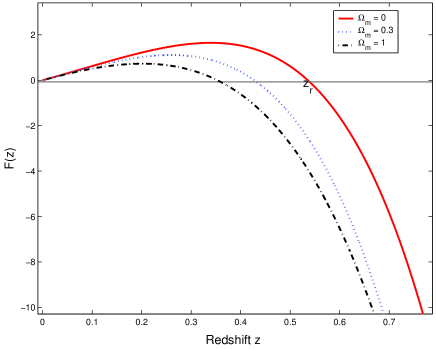
Figure 2 displays the luminosity distance times the present Hubble parameter (IV) for the three cases considered in Fig.1 (we have chosen $\frac{B^{2}}{2a_{o}^{4}b^{2}}=5\times 10^{-3}$). When $z\ll 1$ the leading terms in (45) are $H_{o}d_{L}\simeq z\,(1+\frac{3B_{\bot}^{2}}{a_{o}^{4}b^{2}})$. So the slope at low redshift gets a contribution coming from the background field.

Refer to caption
Figure 2: Luminosity distance times the present Hubble parameter for three different sets of $(\Omega_{m},\Omega_{\Lambda})$ ($\frac{B^{2}}{2a_{o}^{4}b^{2}}=5\times 10^{-3}$).

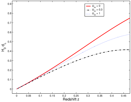
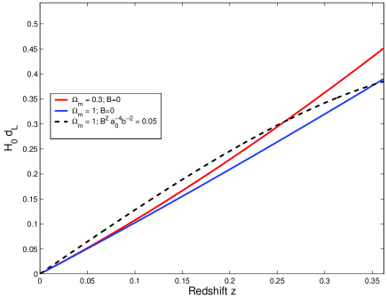
Figure 3 compares the low redshift behavior of standard cosmology ($\Omega_{\Lambda}=0.7$, $\Omega_{m}=0.3$, $b\rightarrow\infty$) with the one of Born-Infeld electrodynamics models without cosmological constant ($\Omega_{m}=1$). Notably the observations $d_{L}$ vs $z$ can be well fitted without using cosmological constant by choosing $\frac{B^{2}}{2a_{o}^{4}b^{2}}\sim 0.05$. In order to better appreciate the role of Born-Infeld electrodynamics in these curves, Fig.3 also includes the curve resulting from an ordinary (Maxwellian) cosmology with $\Omega_{m}=1$.

Refer to caption
Figure 3: Low redshift behaviors of ordinary (Maxwellian) cosmologies (solid lines) compared with Born-Infeld electrodynamics models without cosmological constant.

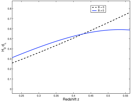
Although non-linear electrodynamics effects could explain the curves of luminosity distance vs redshift for type Ia supernovae Riess-Perlmutter without invoking dark energy, one should be cautious. Accepting a typical value of $10^{-7}G$ pie3 for the cosmological background magnetic field $|{\bf B}_{o}|=B/a_{o}^{2}$ galax , together with the constraint $b\gtrsim 10^{20}V/m$ for the Born-Infeld parameter Jack , then the corrections to the standard cosmology would be negligible. Even so, non-linear electrodynamics should be considered as a source of degeneration in the curve $d_{L}$ vs $z$. Figure 4 compares the curve of the standard cosmology ($\Omega_{m}=0.3$, $\Omega_{\Lambda}=0.7$, $b\rightarrow\infty$) with the one resulting from Born-Infeld electrodynamics for the same values of $\Omega_{m}$ and $\Omega_{\Lambda}$. The curves intersect at $z_{r}=0.43$. If $z<z_{r}$ the curves get their maximum separation at $z=0.26$. If $z>z_{r}$ the luminosity distance predicted by Born-Infeld electrodynamics becomes smaller than the one from standard cosmology. In this last case the curves seem to go dramatically apart (however this feature should be confirmed by extending the calculus up to a higher order of approximation). The degree of separation of both curves is governed by the value of $\frac{B^{2}}{2a_{o}^{4}b^{2}}$. Future observations could allow a test of these features to obtain a constraint for this value.

Refer to caption
Figure 4: Luminosity distance times the present Hubble parameter for $\Omega_{m}=0.3$, $\Omega_{\Lambda}=0.7$. Comparison between Maxwell (dashed line) and Born-Infeld (solid line) electrodynamics ($\frac{B^{2}}{2a_{o}^{4}b^{2}}=5\times 10^{-3}$).

V Conclusions

In this paper we have solved the Born-Infeld equations for electromagnetic plane waves propagating in a background magnetic field. In the absence of a background field, the Born-Infeld plane waves are equal to the Maxwell ones. On the contrary, in the presence of a background magnetic field ${\bf B}$ the non-linear effects modify both the phase and the amplitude of the wave with corrections that depend on the combination $|{\bf B}|^{2}\,a^{-4}\,b^{-2}$, where $a$ is the scale factor of the universe. It is remarkable that Born-Infeld electrodynamics depends on $a$ and $b$ only through the combination $a^{4}b^{2}$. This means that the Maxwellian approximation ($b\rightarrow\infty$) also corresponds to the limit $a\rightarrow\infty$. So, although the electromagnetic field is presently well described by Maxwell equations for a wide range of phenomena, the non-linear Born-Infeld electrodynamics could have an influence in the past when the scale factor was smaller. Therefore the expanding universe is a good laboratory to test Born-Infeld electrodynamics; many non-linear aspects of its equations could be relevant when highly redshifted objects are observed.

In this work we have begun the search for this kind of effects. We found that the influence of Born-Infeld electrodynamics on the luminosity distance (45) exhibits interesting features that could be experimentally established by means of more precise supernova observations and a better knowledge of the cosmological background fields. Firstly, the experimental data for $d_{L}$ vs $z$ could be fitted without invoking dark energy, although there is no observational evidence of the background field that would be required. Secondly, the shape of the curve $d_{L}$ vs $z$ predicted by the standard cosmology ($\Omega_{m}=0.3$, $\Omega_{\Lambda}=0.7$, $b\rightarrow\infty$) for high redshifts differs appreciably from the one predicted by Born-Infeld electrodynamics, which opens the possibility of detecting non-linear electrodynamics effects in a future.

Acknowledgements.
M.A. and G.R.B. are supported by ANPCyT and CONICET graduate scholarships respectively. This work was partially supported by Universidad de Buenos Aires (UBACYT X103) and CONICET (PIP 6332).

References

  • (1) A. G. Riess et al., Astron. J. 116, 1009 (1998), S. Perlmutter et al., Astrophys. J. 517, 565 (1999), A. G. Riess et al., Astrophys. J. 607, 665 (2004).
  • (2) T. Padmanabhan, AIP Conf. Proc. 861, AIP (New York) 2006, p. 179.
  • (3) M. Aiello, G.R. Bengochea and R. Ferraro, Phys. Lett. A 361, 9 (2007).
  • (4) M. Born and L. Infeld, Nature 132, 1004 (1933).
  • (5) M. Born and L. Infeld, Proc. Roy. Soc. (London) 144, 425 (1934).
  • (6) S. Deser, R. Puzalowski, J. Phys. A 13, 2501 (1980).
  • (7) G. Boillat, J. Math. Phys. 11, 941 (1970).
  • (8) E.S. Fradkin and A.A. Tseytlin, Phys. Lett. B 163 (1985), 123. A. Abouelsaood, C. Callan, C. Nappi and S. Yost, Nucl. Phys. B 280 (1987), 599. R.G. Leigh, Mod. Phys. Lett. A 4 (1989), 2767. R.R. Metsaev, M.A. Rahmanov and A.A. Tseytlin, Phys. Lett. B 193 (1987), 207. A.A. Tseytlin, Nuc. Phys. B 501 (1997), 41. A.A. Tseytlin, in The many faces of the superworld, ed. M. Shifman, World Scientific (Singapore) 2000.
  • (9) V. Dyadichev, D. Gal’tsov, A. Zorin and M. Zotov, Phys. Rev. D 65, 084007 (2002). R. García-Salcedo and R. Breton, Int. J. Mod. Phys. A 15, 4341 (2000). M. Sami, N. Dadhich and T. Shiromizu, Phys. Lett. B 568, 118 (2003). E. Elizalde, J. Lidsey, S. Nojiri and S. Odintsov, Phys. Lett. B 574, 1 (2003).
  • (10) J. Plebanski, Lectures on non linear electrodynamics (Nordita Lecture Notes, Copenhagen, 1968).
  • (11) H. Salazar Ibarguen, A. García and J. Plebanski J, Math. Phys. 30, 11 (1989).
  • (12) M. Novello, V. A. De Lorenci, J. M. Salim and R. Klippert, Phys. Rev. D 61, 045001 (2000).
  • (13) M. Novello and J. M. Salim, Phys. Rev. D 63, 083511 (2001).
  • (14) M. Novello and S. E. Perez Bergliaffa, AIP Conf. Proc. 668, 288 (2003).
  • (15) H. Goldstein, C.P. Poole and J.L. Safko, Classical Mechanics,(Addison Wesley, N.Y., 2002).
  • (16) N.D. Birrell and P.C.W. Davies, Quantum Field Theory in Curved Space, (Cambridge University Press, Cambridge, 1984).
  • (17) E. W. Kolb and M. S. Turner, The Early Universe, Chapter 2, (Westview Press, Boulder, 1994).
  • (18) A. Howard and R. Kulsrud, Astrophys. J. 483, 648 (1997), M. Giovannini, Int. J. Mod. Phys. D 13, 391 (2004), P. P. Kronberg, Rep. Prog. Phys. 57, 325 (1994), L. M. Widrow, Rev. Mod. Phys. 74, 775 (2003).
  • (19) J. D. Jackson, Classical Electrodynamics, 3rd. edition, (John Wiley and Sons, N.Y., 1999).
  • (20) In curved space-time, $T_{0}^{\alpha}$ (one covariant index and one contravariant index) coincide with the tensor components in an orthonormalized basis; thus, they effectively give the measure of the energy flux.
  • (21) The approximation is valid when $(1+z)^{4}\,\frac{B_{\bot}^{2}}{a_{o}^{4}b^{2}}\ll 1$; see for instance (35).
  • (22) Notice that the energy density associated to such a field is much smaller than the matter energy density.