RICE Limits on the Diffuse Ultra-High Energy Neutrino Flux

Abstract

We present new limits on ultra-high energy neutrino fluxes above $10^{17}$ eV based on data collected by the Radio Ice Cherenkov Experiment (RICE) at the South Pole from 1999-2005. We discuss estimation of backgrounds, calibration and data analysis algorithms (both on-line and off-line), procedures used for the dedicated neutrino search, and refinements in our Monte Carlo (MC) simulation, including recent in situ measurements of the complex ice dielectric constant. An enlarged data set and a more detailed study of hadronic showers results in a sensitivity improvement of more than one order of magnitude compared to our previously published results. Examination of the full RICE data set yields zero acceptable neutrino candidates, resulting in 95% confidence-level model dependent limits on the flux $E_{\nu}^{2}d\phi/dE_{\nu}<10^{-6}{\rm GeV}/({\rm cm^{2}s~{}sr})$ in the energy range $10^{17}<E_{\nu}<10^{20}$ eV. The new RICE results rule out the most intense flux model projections at 95% confidence level.

^∗Contact for additional information.

I Introduction: UHE Neutrino Physics

The motivation for producing a new map of the Universe, as viewed through neutrino ‘eyes’ is now well-established. Ultra-high energy (“UHE”; E$>$1 PeV) neutrinos point back to sources of high energy cosmic rays, providing a direct picture of the source and the acceleration mechanism. Detection of UHE neutrino fluxes simultaneous with gamma-ray bursts (GRB’s)GRBs could provide essential information on the nature of these extraordinarily luminous sources and help resolve the question of whether GRB’s are responsible for the bulk of the UHE cosmic ray particle flux incident at Earth. In the $10^{18}-10^{20}$ eV energy regime, “GZK” neutrinos may distinguish between source evolution models for UHE cosmic raysSeckelS05 . At even higher energies, “Z-burst” neutrino modelsWeiler have been proposed to explain the $\geq$$10^{20}$ eV cosmic ray flux claimed by the AGASA experimentAGASA98 ; neutrinos may also identify more exotic sources such as topological defectsBerezinsky . In the realm of particle physics, detection of UHE neutrinos from cosmological distances, if accompanied by flavor identification, may permit measurement of neutrino oscillation parameters over a wide range of $\Delta m^{2}$Francis-David-mixing-sensitivity ; Pakvasa03 or observation of $\nu_{\tau}$ via “double-bang” signaturesdoublebang . Additionally, the angular distribution of upward-going neutrino events could be used to measure weak cross-sections at energies unreachable by man-made acceleratorssigma . Alternately, if the high energy weak cross-sections are known, they can be used to test Earth composition models along an arbitrary cross-section, so-called ‘neutrino tomography’tomography .

Several recent projects (AMANDAAMANDA1 , IceCubeIceCube , NESTORNESTOR , NEMONEMO , Lake BaikalBAIKAL , ANTARESAntares , e.g.) have demonstrated photomultiplier-tube based detection of high energy cosmic ray muon neutrinos, by observing the optical Cherenkov cone which results from muons produced in $\nu_{\mu}$ weak current interactions. To detect neutrinos at UHE, it is more effective to exploit coherence of radio Cherenkov emissions. The amplitude of radio frequency signals emitted by neutrino-generated electromagnetic showers in the MHz-GHz regime increases nearly linearly with energy, making radio detection the most efficient scheme presently known at ultra-high energies.

RICE employs this strategy to search for neutrino interactions occurring in cold polar ice, which has exceptional transmission properties favorable for radio detection. Here we extend our previous results astroph-cal ; astroph-results , which were based on shorter running times and less advanced detector response modeling. We report new limits based on additional data and further consideration of systematic errors.

II The RICE Detector

The status of the current array deployment is summarized in Table 1; further details on detector geometry, deployment and calibration procedures are presented elsewhereastroph-cal . The Martin A. Pomerantz Observatory (MAPO) building houses hardware for several experiments, including the RICE and AMANDA surface electronics, and is centered at (x$\sim$40m, y$\sim-30$m) on the surface. The AMANDA array is located approximately 600 m (AMANDA-A) to 2400 m (AMANDA-B) below the RICE array in the ice; the South Pole Air Shower Experiment (SPASE) is located on the surface at (x$\sim$-450m, y$\sim$0m). The planned IceCube experiment will circumscribe the existing AMANDA experiment, with a hexagonal footprint of radius $\sim$500 m and centered approximately 200 m northwest of the origin. The coordinate system conforms to the convention used by the AMANDA experiment: grid North is defined by the Greenwich Meridian.

Channel (Hole)	x- (m)	y- (m)	z- (m)
0 (A11)	4.8	102.8	-166
1 (A6)	-56.3	34.2	-213
2 (A13)	-32.1	77.4	-176
3 (A12)	-61.4	85.3	-103
4 (A6)	-56.3	34.2	-152
5 (A7)	47.7	33.8	-166
6 (B2)	78.0	13.8	-170
7 (B3)	64.1	-18.3	-171
8 (B1)	43.9	7.3	-171
9 (B3)	64.1	-18.3	-120
10 (B1)	43.9	7.3	-120
11 (B4)	67.5	-39.5	-168
12 (A18)	66.3	74.7	-110
13 (A15)	-95.1	-38.3	-105
14 (A16)	-46.7	-86.6	-105
15 (A19)	95.2	12.7	-347
19 (A15)	-95.1	-38.3	-135

Table 1: Location of RICE radio receivers for the bulk of the data relevant to this paper (in Jan. 2004, channel 11 was moved to just below the surface, at a depth of approximately 2 m). We have adopted the coordinate system convention used by the AMANDA collaboration. “A” holes correspond to holes drilled for AMANDA; holes B2 and B4, drilled for RICE in 1998, have been re-opened in subsequent seasons for radioglaciological measurements.

II.1 Radio Cherenkov Detection

Long-wavelength (radio-wave) detection of electromagnetic showers in dense media relies on two fundamental pillars - long attenuation lengths of order 1 km in cold polar ice, and coherence extending up to 1 GHz for radio Cherenkov emission from the net charge developing in showers, as recently verified using data taken in an electron testbeamslac-testbeam ; slac-salt04 . Ultra-high energy showers in dense targets contain roughly one excess electron per four GeV of shower energy, leading to a rapid growth of sensitivity with increasing energy. The ANITAANITA , GLUEGLUE , FORTEFORTE , RAMANDRAMAND , RICEastroph-results ; astroph-cal ; RICEnZ , and SALSASALSA projects all seek radiowave neutrino detection in dense media. Other effortsJonRosner ; LOFAR ; CODALEMA are directed toward radiowave detection of atmospheric cascades. Radio detection schemes have also received considerable attention as probes of monopolesWickWeiler , TeV-scale gravityFeng1 ; Feng2 ; Shahid03 ; Shahid05 ; Pankaj02 , and tau-neutrinosHallsie-2003 .

Discussions of the Askaryan effectAskaryan upon which the radiowave detection technique is founded, its experimental verification in a testbeam environmentslac-testbeam ; slac-salt04 , calculations of the expected radio-frequency signal from a purely electromagnetic showerZHS ; Alvarez-papers ; SoebPRD ; addendum ; RomanJohn , as well as hadronic showersShahid-hadronic , and modifications due to the LPM effectLPM ; spencer04 can be found in the literature. RICE uses its own Monte Carlo-based procedure based on GEANT4-generated showers and charge-by-charge superposition of Cherenkov radio emissionsSoebPRD ; addendum to estimate the signal strength. Several simulationsZHS ; SoebPRD ; Butkevich now give consistent estimates for the expected charge excess, as well as the electric field signal. For frequencies and geometries relevant to RICE, we estimate the uncertainty in the signal field strength, for $f<$1 GHz to be $\lesssim$10%, although errors associated with the LPM effect may be somewhat larger.

Sections III-VII below review calibration of the array, event reconstruction, determination of the effective volume, data acquired and potential events. Section VIII presents the new limits, and sections IX and X present a summary and outlook. Appendices present more details on the calculation of our upper limits, as well as a procedure for deriving the sensitivity of RICE to any arbitrary flux model.

III Current Data Set

The data taken thus far with the RICE array are summarized in Table 2.

	1999	2000	2001	2002	2003	2004	2005	Total
Total RunTime ($10^{6}$ s)	0.18	22.3	4.6	19.9	24.5	11.6	15.1	98.2
Total LiveTime ($10^{6}$ s)	0.10	15.7	3.3	13.6	17.1	9.4	14.9	74.1
DeadTime (303 ON) ($10^{6}$ s)	0.03	3.7	1.0	4.1	5.6	1.1	0.0	15.5
$\geq$4-hit General Triggers ($\times 10^{4}$)	0.26	30.6	6.0	16.9	13.8	9.4	26.5	103.5
Unbiased Triggers ($\times 10^{4}$)		3.3	1.3	3.5	4.4	2.5	4.0	19.0
AMANDA-coincident Triggers ($\times 10^{4}$)	0.064	1.9	2.4	0.016	0.056	0.075	0.002	4.51
SPASE-coincident Triggers ($\times 10^{4}$)		0.48	0.003	0.47	0.021	0.001	0.067	1.04
Veto Triggers ($\times 10^{4}$)	1.2	11182.8	317.4	12973.9	3153.9	142.5	471.0	28242.7

Table 2: Summary of RICE-II data taken through Aug. 15, 2005. Time (303ON) is the total time (in seconds) that the 303 MHz South Pole Station satellite uplink to the LES communications satellite was active and prohibited data-taking. “4-hit Triggers” refer to all events for which there are at least four RICE antennas registering voltages exceeding a pre-set discriminator threshold in a coincidence time comparable to the light transit time across the array ($1.25\mu$s); “Unbiased Triggers” correspond to the total number of events taken at pre-specified intervals and are intended to capture background conditions within the array; “AMANDA-coincident Triggers” correspond to events for which there is at least one RICE antenna hit within $1.25\mu$s of an AMANDA high-multiplicity Optical Module trigger (this trigger has been intermittently disconnected during the course of the experiment when the trigger rate became prohibitively large); “SPASE-coincident Triggers” correspond to events for which there is at least one RICE antenna hit within $1.25\mu$s of a SPASE high-multiplicity surface scintillator trigger and have been used in a search for coincident air shower detections; “Veto Triggers” are events tagged online by a fast ($\sim$10 ms/event) software algorithm as consistent with having a surface origin. Full DAQ readout of such events is heavily pre-scaled, typically by a factor of 10000, to mitigate the compromise in livetime incurred in writing data to disk. Data-taking problems in 2001 resulted in a reduced accumulated livetime for that year.

Over a typical 24-hour period, roughly 1000 data event triggers currently pass a fast online hardware surface-background veto ($\sim$1$\mu$s/event) and an online software surface-background veto ($\sim$10 ms/event). To these data we have applied a sequence of offline cuts to remove background, as detailed later in this document. We determine the efficiency of our event selection criteria using simulations of showers, both electromagnetic and hadronic, resulting from neutrino collisions, superimposed on environment characterization drawn from data itself (unbiased events).

IV Backgrounds

We generally distinguish the different backgrounds to the neutrino search according to the following criteria: a) vertex location of reconstructed source, b) waveform characteristics (time-over-threshold, e.g.) of hit channels, c) goodness-of-fit to a well-constrained single vertex as evidenced by timing residual characteristics (discussed in more detail below), d) RF conditions during data-taking, e) Fourier spectrum of hit channels, f) cleanliness of hits (e.g., presence of multiple pulses in an 8.192 microsecond waveform capture), g) multiplicity of receiver antennas registering hits for a particular event, h) time-since-last-trigger ($\delta t_{ij}\equiv t_{i}-t_{j}$, where $t_{i}$ is the time of the $i^{th}$ trigger and $t_{j}$ is the time of the next trigger. In high-background, low-livetime instances, we expect $\delta t_{ij}\to\delta t_{min}$, where $\delta t_{min}$ is the $\sim$10 s/event readout time of the DAQ. In low-background, high-livetime instances, we expect $\delta t_{ij}\to\delta t_{max}$, where $\delta t_{max}$ is the ten-minute interval between successive unbiased triggers), and i) trigger type fractions. We can coarsely characterize three general classes of backgrounds according to the above scheme, as follows.

1) Continuous wave backgrounds (CW) are expected to have a) a long time-over-threshold for channels with amplitudes well above the discriminator threshold, b) large timing residuals (since the hit times will not be correlated with a single source), c) small values of $\delta t_{ij}$ for the case where the discriminator threshold is far below the CW amplitude, d) backgrounds occurring in all trigger types, since the background will be present in “unbiased” forced-trigger events as well as “general” 4-hit events, e) a Fourier spectrum dominated by one frequency (plus overtones), f) a hit multiplicity which is on average roughly constant, and determined by the number of channels which exceed threshold when their noise voltage is added to the underlying CW voltage. Such backgrounds may cluster in time or show a diurnal periodicity and are generally easily recognized on-line.

2) True thermal noise backgrounds should have a) vertex locations which are spatially distributed as Gaussians centered at the centroid of the array (x=0, y=0, z=–120 m), as demonstrated by Monte Carlo (by simulating four hits at random times within a 1.2$\mu$s discriminator window, roughly corresponding to the light transit time across the array; see Figs. 4 and 5), b) very small time-over-thresholds with signal shapes which are largely indistinguishable from a true neutrino-induced signal – for this reason, thermal noise events satisfying all other kinematic selection criteria are also likely to pass a visual event hand-scan, c) large timing residuals (Fig. 10), d) successive trigger time difference characteristics which depend in a statistically predictable way on the ratio of discriminator thresholds to rms thermal noise voltages, e) a ratio of general/unbiased triggers which, in principle, can be statistically derived from the thermal noise distribution observed in unbiased events, f) a Fourier spectrum dominated by the bandwidth of the various components of a RICE receiver circuit, g) no double pulse characteristics, h) no correlation with date or time. Unbiased events are expected to be representative of the experimental thermal noise ’floor’. In practice, examination of a large number of unbiased events show non-Gaussian tails in a large fraction of the voltage distributions, indicating that there are non-thermal backgrounds present in many of these events.

3) “Loud” transients are observed to constitute the dominant background. We sub-divide possible transient sources into two categories: those sources which originate within the ice itself, primarily due to AMANDA and/or IceCube phototube electronics, and those sources which originate on, or above the surface. Without filtering, the extremely large amplitude radiofrequency transients generated by each AMANDA/IceCube phototube (typically, two km distant and triggering at $\sim 10^{2}$ Hz) would result in a prohibitively large background. After our initial deployment of three test antennas in 1996-97, highpass ($>$250 MHz) filters were inserted to suppress these backgrounds, leaving more sporadic anthropogenic surface-generated noise as the dominant transient background. Such triggers are characterized by: a) typically, large time-over-thresholds, b) $\delta t_{ij}$ distributions which reflect saturation of the DAQ, or show structure if the source is periodic, c) Fourier spectra which are likely to show non-thermal structure.

IV.1 Vertex Suppression of Transient Anthropogenic Backgrounds

Vertex distributions give perhaps the most direct characterization of surface-generated (z$\sim$0) vs. non-surface (and therefore, candidates for more interesting processes) events. Consistency between various source reconstruction algorithms gives confidence that the true source has been located. Due to ray tracing effects, it is difficult to identify surface sources at large polar angles, which increasingly fold into the region around the critical angle. We implement both a “grid”-based vertex search algorithm, as well as an analytic, 4-hit vertex reconstruction algorithm, as detailed previouslyastroph-cal . Once a vertex has been found, one discriminant of “well-reconstructed” vs. “poorly-reconstructed” sources is provided by calculating the average time residual per hit. This is done by: 1) identifying a putative vertex for the event, 2) calculating the expected recorded hit time for each channel assuming that vertex, after taking into account ice-propagation time plus cable delays plus electronics propagation delays at the surface, 3) calculating the difference between the expected time and the actual, measured time, for that reconstructed vertex. That time difference is defined as the “time residual” (as defined for fits to the helical trajectory expected for a charged track traversing a multi-layer drift chamber) for that particular channel. This parameter, when minimized over all channels, defines the reconstructed vertex using the grid-based algorithm. By constrast, the per-channel spatial residual is defined as the distance between the reconstructed vertex when a given channel is included in vertex reconstruction vs. excluded from vertex reconstruction, and is therefore only defined for events with multiplicity greater than or equal to five.

To estimate our ability to correctly reconstruct source vertices, transmitters were placed at various points on the surface, as well as at various depths within the ice, and the reconstructed vertex location compared with the known vertex location. Figure 1 was obtained by broadcasting down to the RICE array from an elevated (z$\sim$+3 m) dipole positioned atop the surveyed AMANDA holes (Table 1), and then reconstructing the source location using our standard timing methods. Our surface source reconstruction resolution within this solid angle is of order 10 m, with poorer longitudinal (vs. lateral) resolution.

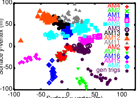
Figure 1: Reconstructed xy-vertices for transmitter data taken with transmitter located above the indicated AMANDA hole, compared with a small sample of general triggers. True source surface coordinates are as indicated in Table I.

To estimate our ability to reconstruct sources at shallow depths (e.g., buried active electronics around South Pole Station), a dipole transmitter was pulsed as it was lowered into a hole in the vicinity of the RICE array (hole B4). Figure 2 shows the result of this exercise, and also illustrates the expected degradation in resolution as z$\to$0. In our subsequent neutrino analysis we require that the reconstructed source depth be greater than 200 m.

Figure 2: Reconstruction of z-coordinate of a transmitter as it is lowered into RICE hole B4. For analytic vertex reconstruction, we assume a constant value of index-of-refraction n=1.

IV.2 Transient and CW Diurnal Backgrounds

We may expect that anthropogenic backgrounds might be periodic with a 24-hour timescale. Figure 3 shows the measured mean rms voltage in three channels as a function of time of day.

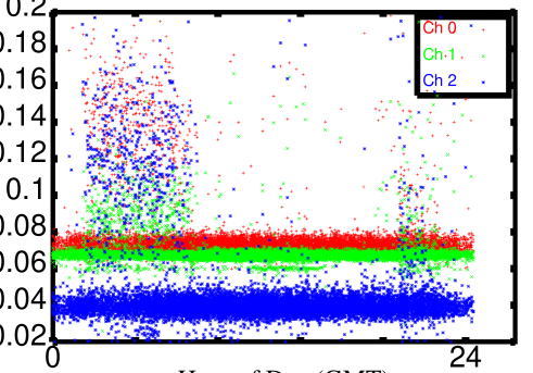
Figure 3: Recorded rms voltage, for three channels, as a function of time of day, for data taken between 1/4/04 and 6/4/04.

There is clear evidence for periodic backgrounds, such as the station satellite uplink during those times when communications satellites are above the horizon, although not all background sources have yet been fully identifiedCorinne-thesis .

IV.3 Thermal Noise backgrounds

When anthropogenic backgrounds are low and the experiment is operating close to the thermal limit, the reconstructed vertex distribution for thermal noise events is expected to peak close to the center of the array, with a width given by the light transit distance across the 1.25 $\mu$s coincidence window defined by the RICE general event trigger. Monte Carlo expectations for the vertex distributions reconstructed from such “thermal events” are shown in Figure 4. By comparison, the vertex distributions for data during a time when the detector was dominated by thermal noise hits (August 2000, as determined by the preponderance of unbiased triggers in those data) are shown in Fig. 5. During the winter months, when station noise is typically lowest, approximately 50% of our backgrounds are thermal noise backgrounds. During the austral summer months, when human activity at South Pole Station is largest, this fraction decreases to less than 10%.

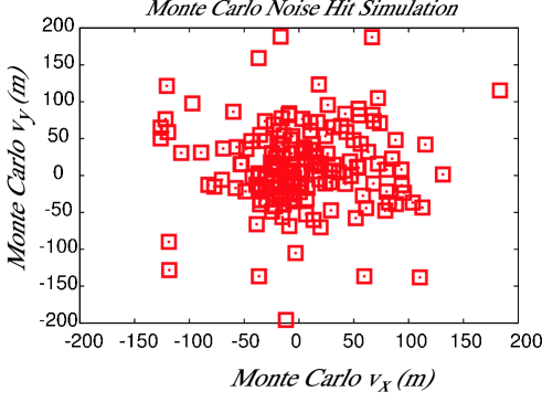
Figure 4: Simulation of x-coordinate of reconstructed vertex ($v_{x}$) vs. y-coordinate ($v_{y}$) of reconstructed vertex for “noise” hits generated in Monte Carlo simulations.

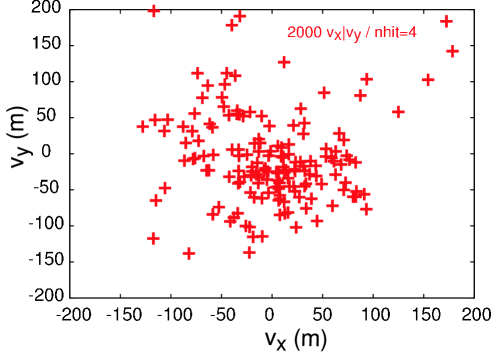
Figure 5: August 2000 data, $v_{x}$ vs. $v_{y}$ vertex distribution, for events having low hit-multiplicity ($N_{hit}$=4) and large time-between-successive-triggers. Events are required to pass initial time-over-threshold requirements.

IV.4 Showers from Atmospheric Muons

High energy muons produced in cosmic ray interactions may penetrate into the ice and suffer catastrophic $dE/dX$ bremsstrahlung or photonuclear interactions. These interactions produce in-ice showers potentially visible to RICE. The magnitude of this background can be estimated from Figs. 3 and 8 of Ref. Thunman . Of interest to RICE, the vertical muon flux above 100 PeV is $E\Phi(E)\sim 2.5\times 10^{-3}({\rm 100~{}PeV}/E_{\mu})^{3}$ km^-2sr^-1yr^-1. The rate increases with zenith angle, roughly as $1/\cos\theta_{z}$. A typical UHE muon is expected to bremsstrahlung one or two photons with $\sim$10% of $E_{\mu}$ over a 1 km track length in ice; at energies above $\sim 200$ PeV photonuclear interactions increase the shower rate. Combining these factors, we estimate that when averaged over the full sky, the integrated rate for shower production with $E_{s}>100$ PeV is a few times 10^-5 km^-3sr^-1yr^-1.

As we show below, the RICE integrated exposure for 100 PeV showers is of order 1 km³sr¹yr¹. Taken together these factors lead us to expect $<$10^-4 muon-induced events in our data sample. Decreasing the energy reduces the experimental sensitivity, whereas increasing the energy reduces the muon flux; at $\sim$100 PeV the RICE response for this signal is maximal.

We note that the estimated rate depends on an uncertain extrapolation of charm hadroproduction cross sections from low energy, and that current experimental bounds allow a flux up to 100 times higher than shown in Ref. Thunman . Still, we expect less than 0.01 events from this source even in the most optimistic scenarios.

IV.5 Atmospheric Neutrinos

Above 1 PeV, the atmospheric neutrino background is also dominated by charm productionThunman . The $\nu_{\mu}$ and $\nu_{e}$ fluxes are slightly larger in magnitude than the atmospheric muon flux. Summing over flavor and averaging over the full sky, we expect a total neutrino flux above 100 PeV of $E\Phi(E)\sim 2\times 10^{-20}({\rm 100~{}PeV}/E)^{3}$ cm^-2sr^-1s^-1. RICE Monte Carlo studies indicate a sensitivity of about $\sim 10^{14}$ cm²sr¹s¹ at 100 PeV. The mismatch between flux and sensitivity ($10^{6}$) is slightly greater than for atmospheric muons. Although a larger fraction of the neutrino energy will be converted to shower energy, only $\sim 10^{-3}$ of the neutrinos interact while passing through the RICE sensitive volume. Even with enhanced charm production we expect no atmospheric neutrino events in the RICE data set. We also note that the RICE effective volume is still small below 10 PeV, so we have very little sensitivity to the Glashow resonance at $E_{\nu_{e}}\sim 6.4$ PeV.

The small fluxes of atmospheric muons and neutrinos above 100 PeV allow RICE to circumvent the primary neutrino backgrounds confronting the optical Cherenkov experiments. However, these small rates also deprive RICE of an obvious calibration ‘beam’.

IV.6 Flaring Solar RF Backgrounds

Radio frequency noise associated with solar activity has been the subject of extensive investigation. Auroral discharges have been continuously monitored in Antarctica in the tens of MHz frequency range, over the last decade. In 2003, there were high-intensity solar flares recorded between Oct. 19, 2003 and Nov. 4, 2003; typically, these result in electrical disturbances on Earth about 24-48 hours later000714 . We have searched for correlations during this time period with high data-taking rates as registered by RICE. We observe no obvious evidence for correlation of our trigger rates with solar flare activityCorinne-thesis .

IV.7 Air Shower Backgrounds

Complementing the production of UHE muons and neutrinos discussed above, there are several possible radio signals associated directly with cosmic ray air showers. These include the production of geo-synchrotron radiation in the atmosphere, as well as transition and Cherenkov signals produced as the shower impacts and evolves into the ice. These three mechanisms all require coherent radiation from all or part of the shower. In all three cases, the transverse profile of the shower dictates a fundamental frequency response, whereas for the geo-synchrotron and Cherenkov signals the shower/observer geometry must also be favorable to have coherent emission from the full longitudinal development of the shower.

Coherent production of synchrotron radiation in the geomagnetic field has recently been observed by the LOPESFalcke05 and CODALEMAArdouin05 collaborations. This signal is most interesting below 100 MHzHuegeF05 , and falls off rapidly in the RICE bandpass. We have not studied this mechanism in detail, but note that the frequency response is ultimately related to the geometry of the air shower – the signal rolls over at $f\sim R/r_{M}^{2}$ where R$\sim$2-3 km is the height of shower max and $r_{M}\sim 100$ m is the Moliere radius for the shower.

Transition radiation results when the shower impacts the icegazazian . In this case, R$\sim$200 m for RICE, f$\sim$200 MHz, and the region for coherent emission is a disk of order 10 m radius. Only a fraction of the excess shower charge is contained within that distance of the shower axis. Further, transition radiation is forward peaked, so illumination of more than one antenna is rather unlikely. We have not seriously modeled transition radiation from air shower impacts as a background for RICE.

The most interesting signal for RICE is the Askaryan pulse produced when the air shower core hits the ice. At RICE frequencies, the Askaryan pulse must originate from a transverse dimension comparable to that for a shower initiated in-ice, a few tens of cm at most. This length scale is compatible with the core of the shower where the highest energy particles reside. Particles have their last interactions of order 1 km above the ice, so the required relativistic-$\gamma$ factor is of order $10^{4}$, corresponding to particle energies $\sim 10$ GeV for $e^{-}$, $e^{+}$ and bremstrahlung $\gamma$’s.

Accordingly, we generated vertical proton showers using the default South Pole configuration of ARIESAIRES , keeping track of all particles reaching the ground with energies greater than 10 GeV. We find that for PeV protons, typically $\sim 3\%$ of the primary energy impacts within 30 cm of the position of the primary axis. This energy is available for producing an Askaryan pulse. We expect that as the primary energy increases a larger fraction of the energy remains in the core, but as we consider less vertical showers, the core will weaken. A rough estimate is that for a pure proton composition the rate of surface showers with energy above 1 EeV is comparable to the rate of 10 EeV primaries averaged over 1 sr, or roughly 0.5 event per km² yr.

We are in the process of enhancing the RICE Monte Carlo to model the modified Askaryan pulses which develop in the low density snow/firn at the surface, and are making the necessary modifications for ray tracing and antenna response in this geometry. Even if the signal is significant, such events may not pass the analysis chain designed largely to eliminate surface noise of anthropogenic origin. We have looked through one year (2002) of dataWahrlich05 , but no clear coincidences with the SPASE array in our SPASE-trigger sample have been observed.

V Detector Calibration and Modeling Details

V.1 Antenna Response

Our current parameterization of the complex RICE dipole response is based on time-domain measurements, in air, of received signals relative to a calibrated standard (Fig. 6).

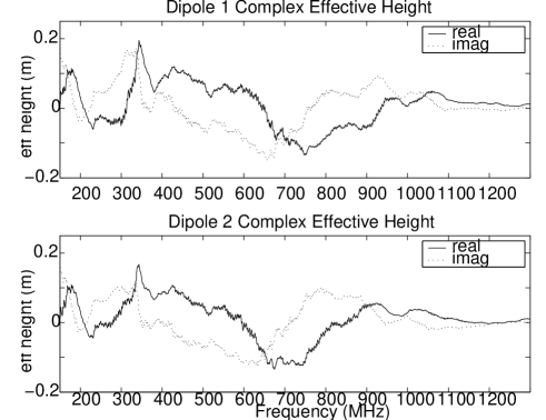
Figure 6: Real and Imaginary parts of RICE complex effective height (in units of meters), measured for two dipole antennas in air.

To scale the antenna characteristics in air (complex effective height ${\vec{h}_{a}}$ and complex impedance ${\vec{Z}_{a}}$) to ice (${\vec{h}_{i}}^{\prime}$ and ${\vec{Z}_{i}}^{\prime}$, respectively), we have used the following procedure: a) assuming that the antenna response is wavelength-dependent only, we shift the frequency dependence of the antenna effective height by the ice index-of-refraction, but assume that the magnitude of the effective height (both real and imaginary components) remains unchanged by the new dielectric environment: ${\vec{h}_{i}}^{\prime}(\omega)={\vec{h}_{a}}(n\omega)$ (the variation of the peak frequency response of the RICE dipoles with frequency has been qualitatively verified by immersing the dipoles in a large sandbox), b) the magnitude of the impedance is reduced by $\sqrt{Re(\epsilon)}$; the frequency dependence is assumed to scale similarly to the effective height ${\vec{Z}_{i}}^{\prime}(\omega)={\vec{Z}_{a}}(n\omega)/n$ (this scaling dependence has been verified using ANSOFT FDTD antenna simulations). The transfer function is now re-calculated, by matching the scaled antenna impedance to the purely real $Z_{c}=50\Omega$ cable load: ${\vec{T}}^{\prime}={\vec{h}_{i}}^{\prime}({\vec{Z}_{c}}/({\vec{Z}_{c}}+{\vec{Z}_{i}}^{\prime}))$.

V.2 Channel-to-Channel Cross-Talk

The possibility of spurious hits appearing in adjacent channels due to cross-talk effects has also been investigated. Such effects are observed in receivers populating the same holes as pulsed transmitters. Based on the non-observation of time-correlated hits in same-hole receivers at the time delays expected from cross-talk, we conclude that the coaxial cable shielding provides good separation between channels.

V.3 Hardware Surface Background Rejection

The only recent notable modification to the RICE data acquisition (DAQ) system is the development, and integration into the DAQ in Jan. 2005, of a Hardware Surface Veto (HSV) board, designed and developed at the KU Instrumentation Design Laboratory. The HSV board is a programmable CAMAC module which compares a time-sequence of antenna hits in a given event trigger with a look-up table of time patterns which correspond to anthropogenic surface noise. The reference look-up table is updated by the winterover at the South Pole on a weekly basis. In the event of an exact (exclusive) match, the trigger is vetoed and the DAQ is reset over the subsequent 1.2 microseconds. The inefficiency of the HSV board has been checked by generating simulated surface source events and determining the fraction which would pass all other neutrino selection criteria. Comparison of the hit patterns for Monte Carlo simulated signal events with the patterns used in our look-up table implies an inefficiency incurred by the HSV board less than 2%.

The utility of the HSV board is assessed numerically by the winter-over at the South Pole on a weekly basis. Runs are taken with the HSV board bypassed and with the HSV board serially inserted into the DAQ chain, in order to determine the enhancement in livetime with the HSV ON. For both HSV-OFF and HSV-ON runs, we tabulate the average livetime (${\cal L}$), as well as the discriminator threshold (${\cal D}$). We assume a disk-like sensitive volume and also that the likelihood of a neutrino at some source point relative to the detector produces a voltage $V$ at an antenna, which must exceed ${\cal D}$ in order to produce hits contributing to the 4-hit trigger, varies inversely with distance, suggesting the ratio ${\cal L}/{\cal D}^{2}$ as a measure of the aggregate neutrino sensitivity. Averaged over year 2005 data-taking, the estimated gain in sensitivity is approximately 40%.

VI Analysis, Monte Carlo simulation and Effective Volume

As described elsewhereastroph-results , the RICE Monte Carlo simulation models the frequency dependence of the width of the Cherenkov cone, ice attenuation effects, antenna response, cable and amplifier response, and the DAQ electronics. Each component in the DAQ chain is characterized on the basis of laboratory, and, where possible, in situ measurements. Thermal noise can be added to each frequency bin assuming that the thermal power magnitude $P_{thermal}$ into the DAQ is given by $P_{thermal}=4k(T_{env}+T_{sys})B\sim V_{thermal}/Z^{2}$, with $B$ the bandwidth of interest and $T_{env}$ ($\sim$220 K) and $T_{sys}$ ($\sim$200 K) the environmental and system temperatures, respectively. The coupling mismatch between the measured antenna impedance and the purely real 50$\Omega$ DAQ impedance prescribes the amount of thermal power delivered from the antenna into the DAQ load; within each frequency bin, the thermal noise amplitude is assigned a random phase prior to summing with the underlying Cherenkov signal amplitude. By Fourier transforming this frequency-dependent signal+noise spectrum in the last step, a time-domain signal is produced which can then be compared to the measured discriminator response to determine if a trigger signal would be generated. Since most neutrinos are at the “edge” of the detectable volume, the calculated effective volume with noise is somewhat larger than the calculated effective volume ignoring noise (more low-sigma signals passing the trigger threshold after adding thermal noise fluctuations than high-sigma signals failing the trigger threshold after subtracting thermal noise fluctuations); for the purposes of setting an upper limit, the Monte Carlo simulation efficiency results presented elsewhere in this paper are based on setting the amplitude of thermal noise to zero. After a simulated event passed this trigger simulation, it was then embedded into an unbiased event and processed through the full event reconstruction, yielding the offline software event detection efficiency $\epsilon$.

The current Monte Carlo simulation improves upon our previous Monte Carlo in several respects: a) the fully complex transfer function (rather than only the real portion of the transfer function) is used in determining the expected signal at the input to the DAQ, b) the current simulation uses GEANT4 results on the expected Cherenkov signal strength from hadronic showers instead of a GEANT3-derived scale factor applied to electromagnetic showersaddendum , c) geometric distortion of the Cherenkov cone due to variation of the index of refraction through the firn is included, and d) ice dielectric effects are now based on in situ measurements recently made at the South PoleRICEnZ ; barwickPole .

VI.1 Signal Shape Modeling

Impulsive neutrino signals yield time-domain responses (“antenna rings”) that are largely insensitive to fine details of the neutrino-induced RF pulse over the RICE frequency bandpass. Antenna rings occur provided the time scale of the neutrino signal is much shorter than the signal decay time in the radio receiver. Event-to-event pulse characteristic variations are largely geometric due to variations in amplitude and shape across the Cherenkov cone, as expected in the single-slit source analogy. Taking two extremes, we have derived the time-domain signals $V(t)$ from an Askaryan-like linearly rising electric field frequency spectrum $E(\omega)$, and from a broad-band spectrum, but falling with frequency. These yield $V(t)$ waveforms nearly indistinguishable in shape. To assess the possible effect on our offline event reconstruction, we have examined four different models (“matched filters”) for the signal shape $V(t)$ expected at the output of the full DAQ chain: a) channel-by-channel signal shapes based on thermal noise ‘hits’ observed in the data, b) channel-by-channel signal shapes based on the data response of each antenna to an englacial radio transmitter, c) channel-by-channel signal shapes based on the response of each antenna to a simulated, short duration neutrino pulse using the expected spectral characteristics of the Askaryan effect, and d) a ‘general’ damped exponential form, which simply requires that a pulse fit the general profile $V(t)=exp(-t/\tau)\cos\omega t$, with $\tau<$30 ns and 100 MHz$<\omega/2\pi<$500 MHz. When applied to a subset of the extant RICE data, the similarity of these various signal parametrizations in identifying hits provides confidence in our antenna calibration and pattern recognition algorithms.

VI.2 Effective Volume ($V_{eff}$) Calculation

The expected detected event rate (${\rm GeV^{-1}}$) can be determined using: $N(detected)=V_{eff}\sigma_{\nu N}{\tt n}\Phi\epsilon{\cal L}\Omega$, where $V_{eff}$ is the energy-dependent effective volume ($m^{3}$), $\sigma_{\nu N}$ is the neutrino-nucleon cross-section ($m^{2}$), $\epsilon$ is the software detection efficiency for an event which is expected to fire the online hardware trigger ($\sim$0.6), n is the number density of targets in the ice ($m^{-3}$), $\Phi$ is the model-dependent flux, expressed as ($N$/(GeV-$m^{2}$s-sr)), $\Omega$ is the sensitive solid angle (sr), and ${\cal L}$ is the livetime. The expected number of detected events can then be compared to the observed number of events; the ratio of these two gives the model-dependent normalization on the flux.

The Monte Carlo effective volume is determined in two steps. First, hadronic and electromagnetic showers are separately simulated over $2\pi$ sr. Since the earth is nearly opaque at these energies, flux from the lower hemisphere has only a small effect on our total effective volume. This contribution to the total effective volume ($\sim$6%) is subsequently ignored. Showers initiated by electrons ($e$) are elongated by the LPM effect, whereas hadronic ($h$) showers initiated by quark jets are not. As a result electron-initiated showers have narrow radiation patterns and exhibit reduced detection efficiency. At a given shower energy, the effective volume is simply calculated as the ratio of the number of Monte Carlo simulated events which produce event triggers in the RICE detector, relative to the total number of simulated events at that energy, multiplied by the total volume sampled: $V_{eff}(E_{shower})=(N^{MC~{}triggers}/N^{MC~{}total~{}events})*V_{0}(E_{shower})$. Since the number of triggers is inversely related to the trigger threshold, our final experimental result must appropriately sum over the effective volumes appropriate for the separate running conditions between 1999 and 2005. Clearly the trigger likelihood will vary as a function of distance – at very close distances, the possibility of simultaneously firing four antennas becomes small due to the cone-like Cherenkov geometry; at large distances, attenuation effects limit the efficiency. Source distributions of generated neutrinos (red dots) compared with reconstructed electromagnetic showers (blue squares) and reconstructed hadronic showers (green crosses) are shown in Figures 7 and 8 for two shower energies. Note that, in the interests of computational execution speed, we have neglected any possible contribution to the numerator ($N^{MC~{}triggers}$) from showers for which the viewing angle, as measured from the center of the array, differs from the Cherenkov angle $\theta_{c}$ by more than 10 degrees ($\approx 1\sigma$ at f=200 MHz). This biases our result to favor those geometries corresponding to “direct hits”, with some underestimate of the total effective volume by ignoring those cases where the array deviates by more than ten degrees from the Cherenkov angle, but the signal strength is otherwise large enough to result in an event trigger. As is evident from the Figures, we also neglect any possible contribution to $V_{eff}$ from the bottom 310 meters of the 2810-m thick South Polar ice sheet, given the expected increased radiofrequency absorption with temperaturebufordkurtT(z) .

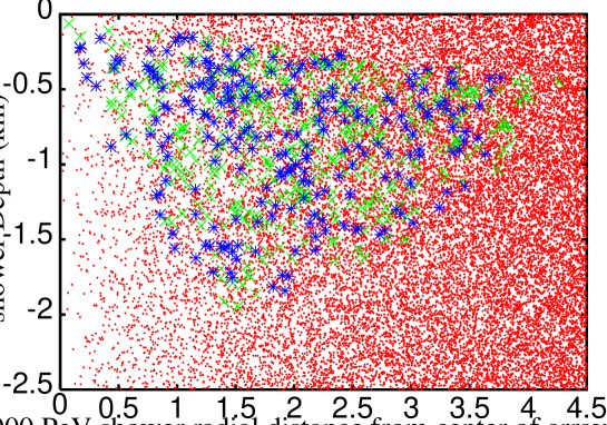
Figure 7: Locations of all simulated neutrino interactions (red points) vs. neutrino interactions producing triggers, for $E_{shower}=1000$ PeV, separately for electromagnetic (blue asterisks) vs. hadronic showers (green crosses), as described in text.

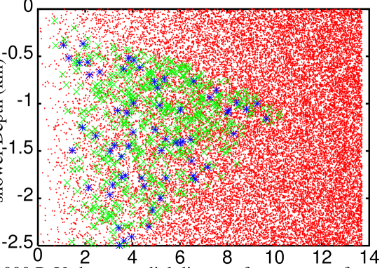
Figure 8: Locations of all simulated neutrino interactions (red points) vs. neutrino interactions producing triggers, for $E_{shower}=10^{5}$ PeV, separately for electromagnetic (blue asterisks) vs. hadronic showers (green crosses), as described in text.

In the second step, the shower-dependent effective volume is re-cast as a neutrino-dependent effective volume. Attenuation and regeneration of neutrinos due to earth absorption effects are simulated separately for $\nu_{e}$, $\nu_{\mu}$ and $\nu_{\tau}$. All flavors of neutrino create $h$-showers as recoil jets in charged (CC) and neutral (NC) current reactions. One flavor ($\nu_{e}$) creates $e$-showers in CC events. For $h$-showers the shower energy is related to the inelasticity $y(E_{\nu})$ and the neutrino energy $E_{\nu}$ by $E_{s}=y(E_{\nu})E_{\nu}$, whereas for $e$-showers in $\nu_{e}$ CC events $E_{s}=(1-y(E_{\nu}))E_{\nu}$. We use isoscalar-target SM cross sections evolved to high energy. The ingredients include the tree-level parton amplitudes and CTEQ 6.2 parton distribution functions, with Q² extrapolation where required. We also include a 20% reduction due to the nuclear (EMC) effects in oxygen. For a given flux model, neutrino mixing is assumed to distribute the total flux equally across all three flavors. Due to the competition between the LPM effect and an average inelasticity of $y\sim 0.2$, for $E_{\nu}<$1 EeV detection of an isoflavor flux is dominated by $e$-showers, whereas $h$-showers dominate above 1 EeV.

VI.3 Event Reconstruction Efficiency $\epsilon$

We determine $\epsilon$ by processing simulated neutrino collision events embedded into data unbiased events. We have selected a background unbiased sample representative of the data comprising the bulk of our accumulated livetime. These Monte Carlo events are subsequently analyzed as real data, and are also tested against the online software veto algorithm. We note that, although full ray-tracing effects are implemented in neutrino event generation, analytic vertex reconstruction currently ignores ray curvatures and assumes straight-line trajectories. Grid-based vertexing properly integrates propagation time over the full in-ice signal trajectory. In our simulation, antenna hit times are smeared by a Gaussian with $\sigma_{t}$=10 ns (consistent with timing resolutions derived from transmitter data, but leading to an overcounting of timing resolution contributions due to hit-recognition uncertainties, after embedding into unbiased events); voltages are smeared by $\pm$3 dB to reflect our canonical gain uncertainty of 6 dB in power. Figure 9 shows a typical simulation vs. data comparison. Plotted is $log_{10}$ of the $\chi^{2}$ Cherenkov cone-fit to the hit channels, assuming either the grid vertex or the 4-hit vertex point.

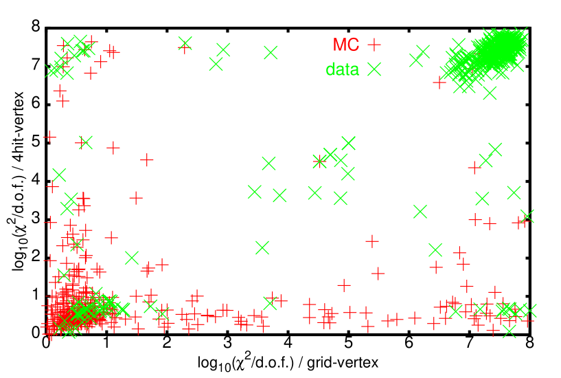
Figure 9: Scatter plot of $\chi^{2}$ for fits that constrain the origin of the Cherenkov cone to the vertex determined using grid-based vertexing algorithm, compared to the vertex found using the analytic “4-hit” vertex algorithm, for events passing initial time-over-threshold and minimum hit multiplicity requirements. Recorded voltages are matched against those expected for a neutrino-induced shower generating a Cherenkov cone, with the apex constrained to a given vertex. The cone width is set to the value expected at the peak of the RICE bandpass ($\sim$300 MHz). We require that either Cherenkov fit satisfy the condition $\chi^{2}/d.o.f.<$50. The more distant the reconstructed vertex, the more difficult it is to discern the curvature of the Cherenkov wavefront, and the smaller the $\chi^{2}$; in such a case, all receivers lie in the same swath of Cherenkov cone.

Similarly, Figure 10 compares the distribution of the total time residual, summed over all hit channels, vs. the time-since-last-trigger for “general” 4-hit triggers (dominated by surface noise), our signal Monte Carlo sample (embedded into unbiased events), and a sample of data events which sets a low threshold (4$\sigma_{rms}$) as a “hit” criterion and therefore preferentially selects thermal noise fluctuations as hits. As expected, the “thermal” sample displays a considerably broader time residual distribution than the MC neutrino sample.

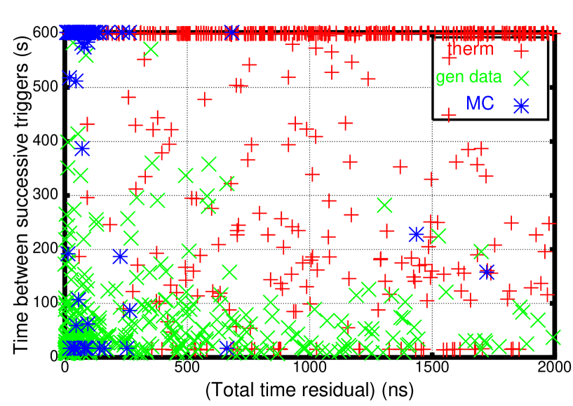
Figure 10: Time residual vs. time-between-successive triggers for MC neutrino simulations, general data triggers, and thermal noise fluctuations. In the absence of an intervening general data trigger, the 10-minute interval between successive forced “unbiased” events is evident in the Figure.

Once initial offline event selection requirements (no channels with time-over-threshold greater than 50 ns, and at least four 5$\sigma$ excursions in an event) are applied in the first pass, data are subjected to more rigorous event selection criteria. This second pass includes additional cuts, after which event waveforms are visually examined (hand-scanning). The effect of the application of the cuts is shown in Table LABEL:tab:cuts; “Data” refer to typical raw data, and “MC” gives the survival rate for events consisting of Monte Carlo simulated signal waveforms superimposed upon the unbiased event ‘environment’. The cut values are obtained by comparing Monte Carlo simulated neutrino events with events tagged as “veto” events by our fast, online software filter based exclusively on discriminator threshold-crossing hit times.

Table 3: Summary of offline Monte Carlo efficiency and cut application. (The online software surface veto- efficiency is estimated to be $90\pm 2$%, and represents an additional multiplicative inefficiency.) For the entries below, Monte Carlo statistical uncertainty is of order 2% (relative). Systematic error on reconstruction efficiency is estimated to be $\sim$20% (relative). Events passing the last requirement are hand-scanned in the final analysis stage.

	MC (%)	MC (%)	Data (%)
	EM	Had
Selection Requirement	showers	shower
1) Initial sample	100	100	100
2) Acceptable Time-Over-Threshold (TOT):	100	100	39.341
3) $\geq$4 $5|\sigma_{rms}|$ hits:	100	100	33.223
4) $\geq$4 $6|\sigma_{rms}|$ hits:	100	100	16.842
5) Double-Pulse Rejection:	99.3	99.0	16.053
6) High quality 3-d vertex:	99.3	98.6	15.657
7) Vertex depth below firn:	89.9	92.8	1.119
8) Acceptable Total Time residuals:	86.5	90.1	0.927
9) Passing tighter Time-Over-Threshold:	84.0	86.0	0.919
10) $\leq$2 hits with large Time residuals:	82.2	83.0	0.855
11) Acceptable Spatial residuals:	81.3	79.4	0.190
12) Satisfying Cherenkov geometry:	74.9	72.1	0.038
13) $\geq$5 $6|\sigma_{rms}|$ hits:	67.4	66.2	0.031

The final hand-scanning stage removes cases where spurious hits (or incorrectly-determined hit times) led to an incorrectly calculated vertex location. At this point, the reconstruction program is fed times for all channels determined through scanning rather than through the software pattern-recognition algorithms. Although the rate of spurious hits is largely antenna-independent, the vertex displacement relative to the true vertex is obviously antenna and geometry-dependent. Channel 15, which is roughly twice as deep as the next-deepest antenna, tends to have disproportionate weight in calculation of the z-vertex of the event. Many of the events remaining, and subsequently discarded, are events for which there was an incorrect hit-time chosen for channel 15 by the pattern-recognition algorithm. The presence of ‘early’ hits in the near-surface channels, not used in vertex reconstruction, but evident in scanning, is also used as a criterion for rejecting events of surface origin. We assume hand-scanning incurs no additional inefficiency in estimating $\epsilon$.

No events survive as in-ice shower candidates. An example of an event which survived initial software requirements, but was later discarded, is shown in Figure 11. For this event, the reconstructed z-vertex was just below our nominal cut, however, an examination of the waveforms shows an early hit in channel 11 (points) at a time approximately $1.6\mu$s prior to hits recorded in the deeper channels 6, 8 and 14. Given the smaller cable delay in channel 11 relative to the other channels ($\sim$500-700 ns) and the additional light transit time for a source generated at the surface to reach the deeper channels ($\sim$750-1000 ns), we conclude that this waveform pattern is consistent with surface-generated backgrounds.

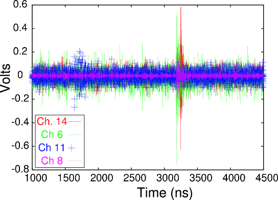
Figure 11: Event surviving up to hand-scan, but rejected on the basis of early hit in channel 11.

VII Systematic Uncertainties

Our flux limit is derived directly from the effective volume $V_{eff}$, the livetime ${\cal L}$, and the event-finding efficiency $\epsilon(\sim$0.6), which is the product of the online software veto ($\epsilon_{online}\sim$0.9) and the offline software veto listed in Table LABEL:tab:cuts ($\epsilon_{offline}\sim$0.67). In addition to the aforementioned uncertainty in the estimated signal strength produced by a neutrino interaction ($\lesssim$10%), we have considered several other possible systematic errors, as detailed below.

VII.1 Individual Hit Recognition and Event Reconstruction

Inaccurate hit-finding will result in events likely to fail our vertex and time-residual requirements. To verify our hit-finding algorithms, we have compared the results for several different hit-definition criteria: a) the maximum voltage excursion in a waveform, b) the first 6$\sigma$ excursion in a waveform, c) the time that gives the best match to one of four ‘matched filters’ (described above). For simplicity, we have used as a default option b), although all algorithms give essentially the same result. Note that the effect of spurious hits is built into the inefficiency we quote in our Monte Carlo simulations, which also include spurious hits in the unbiased events into which simulated showers are embedded. Once four hits are found, a 3-dimensional vertex is constructed. Vertex reconstruction is observed to work well for in-ice sources close to the array, as calibrated using englacial transmitters. For sources well outside the array, Monte Carlo simulations of neutrinos indicate that although directions are generally well-reconstructed (typical angular deviations between the true and reconstructed angle to vertex are of order $\delta(\theta_{true},\theta_{reconstructed})\ll$0.2), source depths are generally reconstructed closer to the array than simulated. This results in an inefficiency in those cases where the true depth is close to the minimum source depth criterion (200 m). Events at distances $\gtrsim$500 m (which constitute the bulk of our sensitive volume) are not assumed to have well-determined radii, nor are distances to the events needed for the present analysis.

We assess an overall event reconstruction efficiency uncertainty of 20%, based on the limited statistics of our Monte Carlo simulation, as well as the variation observed for Monte Carlo simulations based on different hit-finding algorithms and using different unbiased event samples.

VII.2 Ray Tracing and Index-of-Refraction

Since many of our receivers are located in the firn, radio wavefronts will follow curved rather than direct-line trajectories, depending on the index-of-refraction profile, as discussed elsewhereRICEnZ . This has two significant consequences: a) for Cherenkov radiation incident at nearly horizontal angles, and angles slightly below the horizon ($\theta\approx\pi/2$), antennas in the “shadow zone” will not register hits, resulting in a loss of effective volume. Although initially directed at the receiver shown, ray 1 in Figure 12 is refracted downwards due to the gradient in the $n(z)$ profile. b) Due to curvature effects in the firn, a neutrino interaction below a RICE antenna will, in general, have both a “direct” hit, as well as an “indirect” hit (rays 2 and 3 in the Figure). For the case where ray 3 emerges from the neutrino interaction point at the Cherenkov angle, ray 2 emerges with an angle greater than the Cherenkov angle, with a correspondingly diminished electric field strength. However, in roughly half the possible cases, ray 3 will emerge at an angle somewhat smaller than $\theta_{c}$, with ray 2 along $\theta_{c}$, resulting in a significant signal from ray 2 due to refractive effects of the firn. In our Monte Carlo simulation, we now include loss of effective volume due to shadow-zone effects. We have not included the expected positive enhancement in $V_{eff}$ due to “second-ray” effects just discussed in our overall systematic error.

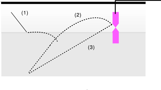
Figure 12: Illustration of ray tracing, and possible refractive effects (ray 2), as described in text. Dotted lines indicate possible rays emanating from a neutrino interaction point.

An additional possible increase in effective volume is due to the focusing of rays, particularly around caustics. This has not been evaluated numerically and is also not included in our current calculations.

Neglecting the indirect-hit contributions discussed above, uncertainties in the real portion of the dielectric constant are explicitly evaluated by comparing the effective volumes using two different models for the index-of-refraction profile $n(z)$. In Figure 13, “Test” refers to an extreme n(z) profile, inspired by different measurements of Antarctic ice properties; “default” is the profile measured at South PoleRICEnZ .

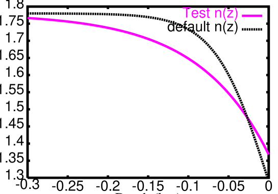
Figure 13: Comparison of test profile for index-of-refraction at South Pole with the current RICE default. Former is used to assess systematic error due to n(z) uncertainties.

Figure 14 shows the relative $V_{eff}$ obtained using the test n(z) (“worst case”) vs. $V_{eff}$ obtained without ray tracing (“best case”). The effect is largest at high energies where trajectories are longest and ray tracing effects are most important.

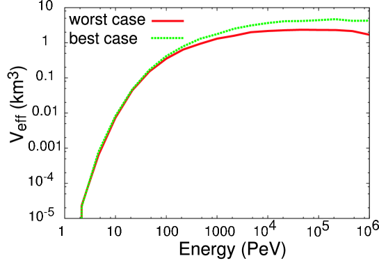
Figure 14: Comparison of relative effective volume (EM showers), obtained without ray tracing and “worst-case” (“Test n(z)” in previous Figure) variation in index-of-refraction profile, as a function of depth. Differences are due to fraction of volume lying in the “shadow” region.

For in-ice sources, the effect of ray tracing corrections on $\epsilon$ is found to be not large, since vertex reconstruction is based on differences of hit times between pairs of hit antennas, rather than the absolute transit times from source location to the antennas themselves. Figure 15 shows the time differences between antenna hits ($\delta(t_{i}-t_{j}$)) for channels i and j, vs. the same quantity for channels i and k ($\delta(t_{i}-t_{k})$) for all possible combinations having $i=0$ or $i=1$. In the Figure, large crosses indicate time differences obtained without ray tracing, nearby smaller “x” symbols indicate time differences for the same ensemble of events obtained with ray tracing. Ray tracing introduces a typical correction of order 5 ns, or half of our quoted hit time uncertainty.

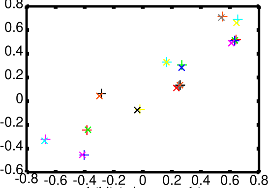
Figure 15: Hit Time differences with (“+”) and without (“x”) ray tracing corrections for channels 0 and 1 (selected at random).

VII.3 Attenuation Length

As discussed and numerically estimated in our previous publication, attenuation length uncertainties become significant at high energies. The corresponding energy dependent error in $V_{eff}$ is folded into our overall systematic error, using the $\pm 1\sigma$ error bars quoted in the attenuation length measurement made at the South Pole in 2004barwickPole .

VII.4 Transfer Function

VII.4.1 Dipole-to-Dipole Uncertainties

These are estimated by comparing the transfer functions measured for several dipoles. We observe variations in the transfer function of order 5-10% in magnitude, as a function of frequency, resulting in a relatively small, and symmetric effect on the calculated neutrino effective volume.

VII.4.2 Transfer Function scaling from air to ice

To take into account possible uncertainties in our scaling from air to ice, we have compared the effective volume using the scaling described previously (Section V.1) to a more extreme scaling where the transfer function is simply obtained using: $T_{ice}^{\prime}(\omega)=nT_{a}(n\omega)$, neglecting the complex nature of the transfer function, and assuming that the antenna is perfectly matched to the cable. Figure 16 shows the ratio of the effective volumes calculated using these two different prescriptions. This ratio is folded directly into our overall relative systematic error. For $E_{\nu}>$100 PeV, corresponding to the energy region comprising our greatest effective volume, the effect is not substantial ($\lesssim$5%). For lower energies, the effect can be considerable, reflecting the evolution from an $r^{3}$ sensitive volume to an $r^{2}$ volume.

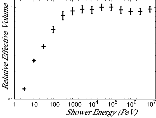
Figure 16: Effective Volume dependence on assumed form of transfer function. Shown is the ratio of effective volumes (note log y-scale) calculated using an impedance-matching model for evolving the transfer function in air to ice, as done in the current RICE Monte Carlo simulation, relative to a simple scaling $T_{ice}^{\prime}(\omega)=nT_{air}(n\omega)$. For E$>$1000 PeV, this ratio plateaus at a value close to unity.

VII.5 Livetime

Livetime is calculated online from measurements of the deadtime incurred per surface veto and also the deadtime incurred per recorded event. We estimate uncertainties in deadtime to be less than 5%.

VII.6 Total Gain

The nominal gain uncertainty of $\pm$6 dB in power, although important at low $E_{\nu}$, becomes less important at high energies, where ice absorption effects are dominant. The stability of the gain of each channel, as a function of frequency, is monitored online. Figure 17 shows the gains for three sample channels (2002 data), corrected for cable and insertion losses, but not low-pass filtering.

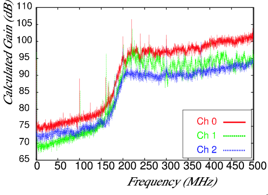
Figure 17: Sample channel gains (2002 data). Smaller calculated gain at low frequencies is due to explicit filtering of low-frequency backgrounds due to the AMANDA experiment, not corrected for in this calculation.

To qualitatively assess the possible implications for our effective volume, we have run our Monte Carlo code with our current default amplifier settings (in the interests of a conservative upper limit, set to $\sim$90 dB for each channel, slightly below in situ calibration in the RICE bandpass, as shown in Fig. 17) vs. the August, 2000 amplifier settings, which were individually tuned, channel-by-channel to give approximately equal contributions (for each channel) to the overall discriminator hit rate. To achieve this equality, gains were turned down in the August, 2000 data sample by as much as 30 dB. For large $E_{\nu}$, the resulting variation in effective volume is of order 20%.

VII.7 Birefringence

The possibility of ice birefringence has been consideredbirefs , although there is no evidence to our knowledge for birefringence of South Polar ice. We have not observed double reception of transmitted pulses or anthroprogenic noise of mixed polarizationRICEnZ . Non-zero birefringence would lead to an asynchronous antenna arrival time of the horizontal- vs. vertical-polarization signal components ($\sim$25 ns for a source 1 km distant), resulting in an average loss of signal strength by a factor $1/\sqrt{2}$ for an antenna sensitive to all polarizations. Since the RICE dipoles are sensitive to only vertical polarizations, birefringent effects will not result in an expected loss of effective volume.

VII.8 Final $V_{eff}$ and associated systematic uncertainty

Figure 18 shows our current effective volume based on electromagnetic and hadronic showers, with $\pm$1-sigma error bars, reflecting the above systematic errors. At very high energies, our new central value is approximately a factor of two smaller than the estimate in our previous publication, although we again point out that we have purposely excluded possible gains in $V_{eff}$ due to a variety of effects. Since systematic errors are not explicitly included in calculation of upper limits, we caution that our quoted sensitivity has large attendant uncertainties. Systematic errors in effective volume, as indicated in Figure 18 result in roughly a factor of two possible variation in the expected overall neutrino event yield.

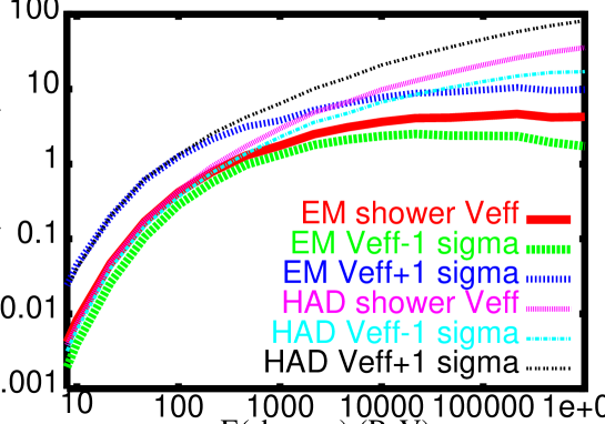
Figure 18: Current effective volume for electromagnetic showers (including LPM effects), and also hadronic showers, with $\pm$1-$\sigma$ systematic errors, as indicated.

VIII Neutrino Flux Limit Results

Our 95% C.L. bounds on representative $\nu$-flux models are shown in Fig. 19. The illustrative AGN models are ruled out at 95% C.L., but the Waxman-Bahcall modelwb is below our limits. The GZKgzk flux models differ substantially. ESSess and PJpj , keyed to models of the stellar formation rate, are below the RICE sensitivity. The KKSSkkss flux, constructed to saturate bounds derived from EGRET observations, is just barely consistent with our 95% C.L. limit, i.e. RICE should have detected 2 events for this model but observed none. Also depicted are 95% C.L. upper limits on diffuse neutrino fluxes predicted by representative GRB models.

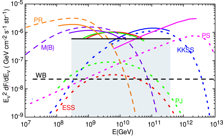
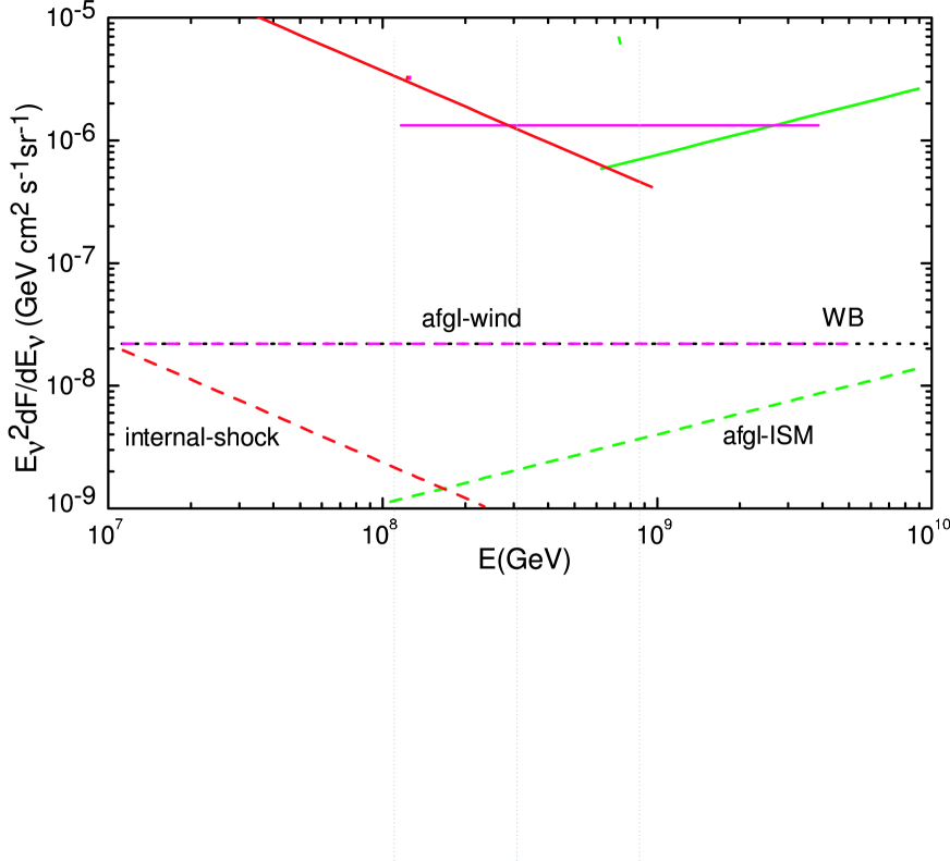
Figure 19: (Top) Upper bounds on total (all flavor) neutrino fluxes for AGN models of PRpr and MB mb , GZKgzk neutrino models of ESSess , PJpj , and KKSSkkss , and the topological defect model of PSps , due to all flavor NC+CC interactions, based on 1999-2005 RICE livetime of about 20500 hrs. Dashed curves are for model fluxes and the thick curves are the corresponding bounds. The energy range covered by a bound represents the central 80% of the event rate. (Bottom) Bounds on diffuse neutrino fluxes from GRBs derived from RICE data. The bounds are for the internal shock wbinsh , afterglow-ISM wbism , and afterglow-wind dailuwind neutrino flux models assuming an isoflavor mixture at the detector; we use updated results soebgrbnu for the fluxes. Systematic errors have not been folded into calculation of upper limits.

To facilitate application of our null search to any other possible related search, Figure 20 shows the livetime-weighted effective volume (${\cal V}$, with units ${\rm cm^{3}}$-sr-yr), as a function of energy. The y-scale for ‘hadronic’ (dashed) and ‘electromagnetic’ (dotted) curves is on the left y-axis of the Figure; these two curves show the RICE effective volume integrated over time (1999-2005) and multiplied by a factor of $2\pi$ steradian, plotted as a function of shower energy. The difference between ‘hadronic’ and ‘electromagnetic’ curves is due to the LPM effect. The exposure ${\cal A}$ is indicated by the y-scale for the solid curve (right, with units cm²-s-sr) and includes standard model NC and CC cross sections convolved with the effective volume (separately for hadronic vs. electromagnetic cases) under the assumption that 1/3 of the total neutrino flux is $\nu_{e}$. Additional details on ${\cal V}$ and ${\cal A}$, as well as the procedure for deriving a predicted RICE observed event yield given an arbitrary flux model, are presented in the accompanying Appendix I.

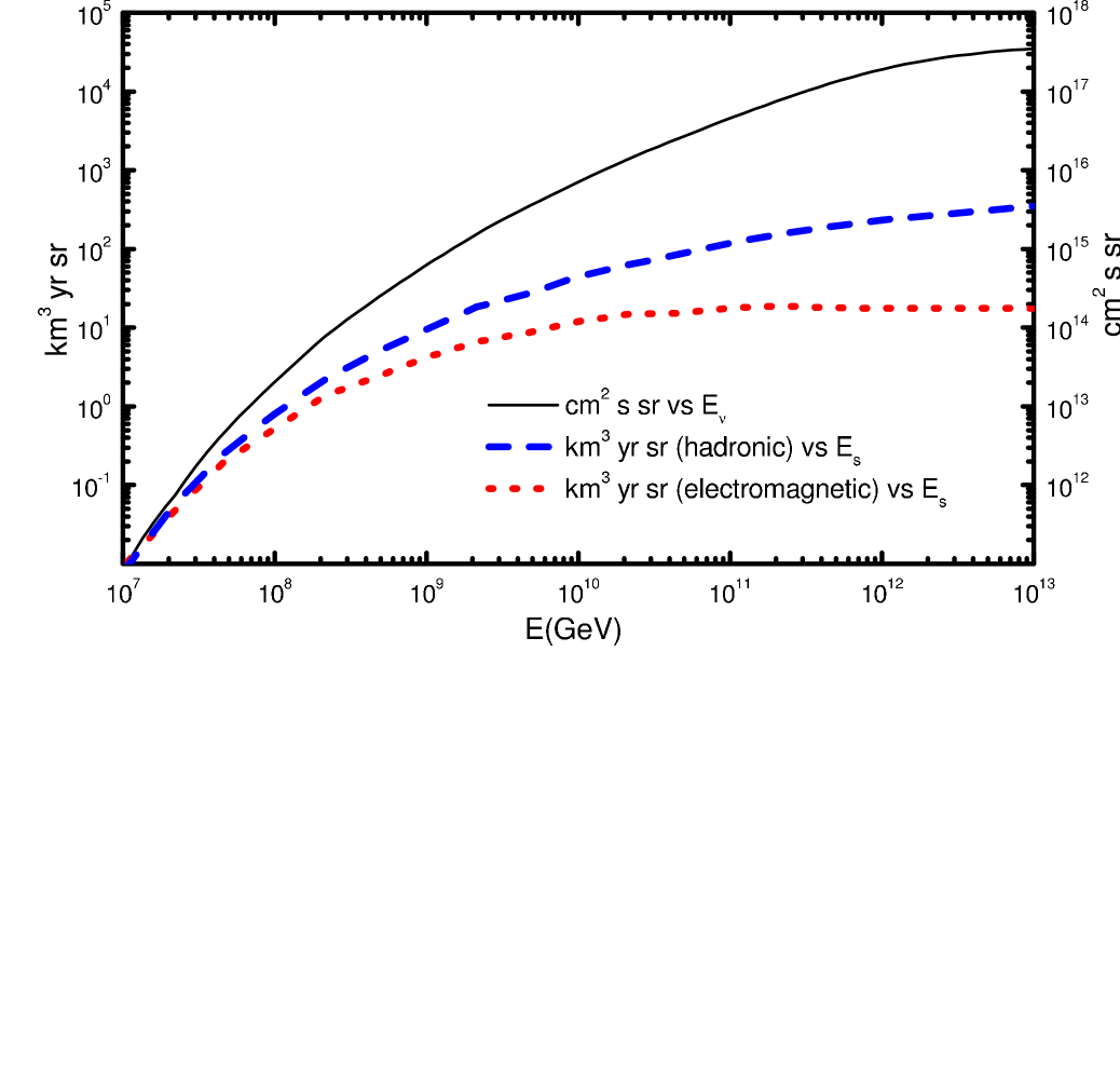
Figure 20: Left scale: Product of $V_{eff}\times Livetime$, as a function of energy. Given an input flux ($N/(cm^{2}-sec-sr)$), and a scattering cross-section (and inelasticity) for any process ($\nu+N\to$electromagnetic shower, $\nu+N\to$hadronic shower, $\nu+N\to\mu$-black-hole$\to$hadronic shower, etc.), one can derive limits on putative cosmic ray fluxes. The RICE-specific event reconstruction efficiency has already been folded into these curves, and can therefore be directly convolved with a given input flux to yield an expected number of events. Right scale: Exposure (${\cal A}$); see text for details.

Although the exposure illustrated in Fig. 20 allows for a comparison of models and experiments, it is often desirable to show the flux limits from an experiment in a model-independent way, as in Fig. 21. The procedures used to derive these limits are discussed in Appendix II. The bold curve is our best model-independent summary of the current RICE results for ‘typical astrophysics’ models. The dashed curve represents the envelope of limits for pure power law models. The three dotted curves are limits based on logarthmic energy binsAnchordoquiFGS02 ; GorhamHNLSW04 .

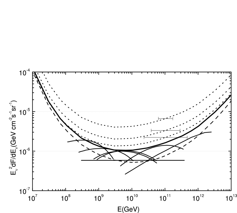
Figure 21: Model-independent limits for the RICE experiment superimposed on model-dependent limits. See Appendix II for discussion.

IX Summary

Using the full dataset accumulated thus far (1999-2005), we have presented upper limits on the incident neutrino flux. Despite suboptimal dense-packing of the array, RICE provides superior sensitivity in the energy regime between $10^{17}-10^{20}$ eV. Limits are considerably stronger than previously reported values, and the most intense flux model projections are ruled out at 95% confidence level.

X Further Work and Future Plans

RICE was originally conceived as a detection system with $km^{3}$ effective volumes per antenna in the PeV domainFMR . Multi-$km^{3}$ effective volume has been achieved at much higher energies, where fluxes are expected to be much lower. Future gains in sensitivity will be realized by improvements to several factors now limiting performance: (1) Limited bandwidth of the current experiment arising from cable losses at high frequencies and the 500 MHz bandwidth of the digital oscilloscopes will be improved with high-bandwidth optical fiber signal transmission and custom surface digitizer boards, 2) A local hardware coincidence multiplicity trigger, which only considers “hits” for which a local antenna cluster (consisting of 4 antennas) itself satisfies a trigger coincidence inconsistent with down-coming signals will result in enhanced online background rejection. As a result, we will greatly improve broad-spectrum energy response by reducing trigger thresholds from the simple one-tier trigger system currently in place. (3) Improvements in geometric lever-arm and the detector footprint beyond that of AMANDA/IceCube will enhance long-ranged vertex sensitivity. During the austral summer of 2005-06, initial deployments of the next generation of neutrino detection hardware are being made at the South Pole. Details on the hardware itself, as well as the 05-06 deployment, are available from KUIDL .

Studies of an expanded radio array are ongoing. Other technologies that hinge on coherence (acoustic detection of showers, e.g.) are also now being explored by other experimental groupsLearned-acoustic ; SAUND ; Rolf&Sebastian ; Buford-acoustic , and an in situ measurement of the acoustic attenuation length at the South Pole is now in progress. Preliminary results of the physics potential of a combined radio plus acoustic detector in conjunction with the IceCube array have recently been discussedRolf&Sebastian ; statistically significant detections of GZK neutrinos (per year) can be realized at relatively modest costs.

XI Acknowledgments

We gratefully acknowledge the generous logistical support of the AMANDA and SPASE Collaborations (without whom this work would not have been possible), the National Science Foundation Office of Polar Programs, the University of Kansas, the University of Canterbury Marsden Foundation, and the Cottrell Research Corporation for their generous financial support. Alexey Provorov and Igor Zheleznykh (Moscow Institute of Nuclear Research, Moscow, Russia) constructed the TEM horn antennas currently used as part of the surface-noise veto. Derek Boyd performed important checks of the overall system timing calibration. John Paden and Matt Peters provided essential antenna expertise. George M. Frichter, Adrienne Juett, Tim Miller, Dave Schmitz, and Glenn Spiczak all performed essential work in the initial construction phases of this experiment. We also thank the winterovers who staffed the experiment during the last six years at the South Pole (Xinhua Bai, Allan Baker, Mike Boyce, Phil Broughton, Christina Hammock, Marc Hellwig, Matthias Leupold, Karl Mueller, Michael Offenbacher, Katherine Rawlins, Steffen Richter and Darryn Schneider), as well as the excellent on-site support offered by Raytheon Polar Services logistical personnel (particularly Rev. Al Baker, Jack Corbin, Joe Crane and Paul Sullivan).

*Appendix I) Calculating upper limits from RICE livetime ${\cal L}$ and $V_{eff}$ (Figure 20)

Determination of ${\cal V}$

The ‘hadronic’ (dashed) and ‘electromagnetic’ (dotted) curves shown in Figure 20 are derived as follows: One computes the effective volume for downward neutrinos using the standard RICE MC simulation (accessible from http://kuhep4.phsx.ku.edu/~iceman) separately for electromagnetic and hadronic showers for different discriminator thresholds. The output is then integrated over time (weighted by the amount of data taken at each given discriminator setting) to obtain a quantity with units (km³yr) as a function of shower energy. This result is then multiplied by $2\pi$ sr (for down-coming neutrinos) to obtain a quantity with units (km³yr-sr), defined as ${\cal V}(E_{shower})$.

Converting from [km³yr-sr] to exposure [cm²s-sr] ($\equiv{\cal A}$)

We convert ${\cal V}(E_{shower})$ to ${\cal A}(E_{\nu})$ as follows:

$${\cal A}(E_{\nu})=\epsilon C_{EMC}N_{A}\rho\left[\begin{array}[]{c}\int_{y_{0}}^{1}dy\frac{d\sigma^{NC}}{dy}VT_{hd}(yE_{\nu})+\frac{2}{3}\int_{y_{0}}^{1}dy\frac{d\sigma^{CC}}{dy}VT_{hd}(yE_{\nu})\\ +\frac{1}{3}\int_{0}^{1}dy\frac{d\sigma^{CC}}{dy}\left(VT_{hd}(yE_{\nu})+VT_{em}((1-y)E_{\nu})\right)\end{array}\right],$$

where $\epsilon$ is the detector efficiency (0.6 for our case); $C_{EMC}$ (=0.8) is a constant factor used to account for the reduction in neutrino-nucleon cross sections in oxygen target as opposed to a nucleon target; $N_{A}\rho$ is Avogadro’s number multiplied by the density of ice (0.92 g/cm³) which gives total number of target nucleons per unit volume; $y$ is the inelasticity of the interaction, and $\frac{d\sigma^{NC}}{dy}$ and $\frac{d\sigma^{CC}}{dy}$ are the neutrino-nucleon neutral current (NC) and charged current (CC) differential cross sections, respectively, in the Standard Model. There are three integral terms. The first term accounts for the contribution from the NC interactions and is the same for all neutrino flavors; $y_{0}$ is the lower limit on the integral and is due to the finite threshold of the detector. The second term is due to CC interactions of $\nu_{\mu}$ and/or $\nu_{\tau}$. The third term is due to the CC interactions of $\nu_{e}$. We treat $\nu_{e}$ CC interactions separately since both the hadronic and the leptonic parts of the final products contribute to shower development in ice; this is not the case for the other two flavors where the lepton does not contribute to the shower. The factors $\frac{2}{3}$ and $\frac{1}{3}$ are due to the isoflavor assumption of the model flux, namely, $\nu_{e}:(\nu_{\mu}+\nu_{\tau})::1:2$.

Significance of ${\cal V}(E_{s})$ and ${\cal A}(E_{\nu})$:

The quantity ${\cal A}(E_{\nu})$, when multiplied with a given model flux d$\phi$/dE_ν, and then integrated over E_ν, gives the expected observed event rate for 1999-2005 RICE operation. This, in turn, implies bounds on that model flux under the assumption of the Standard Model neutrino-nucleon interactions. The quantity ${\cal V}(E_{s})$ thus gives one freedom to use one’s own model for the neutrino-nucleon interactions and then calculate ${\cal A}(E_{\nu})$ using the equation above.

*Appendix II. Model-Independent Neutrino Flux Limits

The expected number of events observed in an experiment is given by $N=\int\phi{\cal A}dE$, where $\phi$ is the flux and ${\cal A}$ is the exposure given in units of area $\times$ solid angle $\times$ time. If no events are observed, then the 95% upper limit constraint $N<3$ places limits on possible flux models. Such model-dependent limits are illustrated in Fig. 19. Since it is exhausting to enumerate all models, it is convenient to provide a model-independent picture of the strength of an experiment. Such model-independent approaches can also be used to compare experiments without the bias of choosing a particular model which may favor one experiment over another.

UHE neutrino astrophysics experiments generally have the following common properties: a) the exposure increases with energy, b) the flux decreases with energy, c) there is almost always a broad intermediate energy regime which dominates the event integral $N$. It is useful to consider power law models where $\phi\sim E^{s}$ and ${\cal A}\sim E^{r}$. Then the integral behaves as $N\sim E^{t}$, where $t=1+r+s$ depends on the combined power laws of flux and exposure. If $t>0$ then $N$ is dominated by high energies, and if $t<0$ it is dominated by low energies. In practice, $t>0$ at low energies due to the increase in ${\cal A}$, but at higher energies ${\cal A}$ saturates and the flux decreases so that $t<0$. In these circumstances, the event rate is dominated by the intermediate energy range around $E_{0}$, defined by the point where $t=0$, or $r+s=-1$.

One can make an estimate of the event integral by expanding the event spectrum around $E_{0}$. It is convenient to introduce several quantities. Define the event spectrum by $g(E)=\phi{\cal A}$. The scaled energy and event spectrum are $y=E/E_{0}$ and $f(y)=g(yE_{0})/g(E_{0})$. The corresponding logarthmic quantities (motivated by the discussion of power law spectra) are $\eta=\log y$ and $\psi=\log f$. Accordingly, we define an energy dependent exponent $\alpha=d\psi/d\eta=(y/f)df/dy$ and an $E_{0}$ dependent exponent $\beta=\psi/\eta$, i.e. $f=y^{\beta}$. With these definitions, $N$ can be written as

$$N = \int g(E)dE=g_{0}E_{0}\Delta$$ (1)

$$\Delta = \int f(y)dy=\int e^{\psi+\eta}d\eta.$$ (2)

The $\Delta$ integral is dominated by the region around $E_{0}$, or equivalently the region near $\eta=0$. In this region, $f\sim 1/y$ or $e^{\psi+\eta}=1$. Thus, $\Delta$ is the effective range of $\eta$ where the event spectrum may be approximated by $1/E$.

It remains to estimate $\Delta$. Using the definition $\beta=\psi/\eta$ and performing a Taylor expansion around $\eta=0$, the integral can be recast as $\Delta=\int e^{(1+\beta)\eta}d\eta=\int e^{(1+\beta_{0}+\beta^{\prime}_{0}\eta)\eta}d\eta$, where the subscripts denote evaluation at $\eta=0$ and the ^′ denotes $d/d\eta$. Using L’Hopital’s rule $\beta_{0}={{\rm Lim}\above 0.0pt{\eta\rightarrow 0}}\frac{\psi}{\eta}=\psi^{\prime}=\alpha(E_{0})=-1$, and $\beta^{\prime}_{0}={\rm Lim\above 0.0pt\eta\rightarrow 0}(\psi^{\prime}-\frac{\psi}{\eta})^{\prime}/\eta^{\prime}=\alpha^{\prime}(E_{0})-\beta^{\prime}_{0}$, or $\beta^{\prime}_{0}=\alpha^{\prime}_{0}/2$. Using these results in the approximation for $\Delta$, one finds

$$\Delta\simeq\int e^{\frac{\alpha^{\prime}_{0}}{2}\eta^{2}}d\eta=\sqrt{\frac{2\pi}{\alpha^{\prime}_{0}}}.$$ (3)

Once $\alpha^{\prime}$ and $\Delta$ are determined, the 95% c.l. model-independent flux limit for no observed events is given by

$$\phi_{\rm mi}(E)=3\sqrt{\frac{\alpha^{\prime}}{2\pi}}\frac{1}{E{\cal A}}$$ (4)

In principle, $\alpha^{\prime}$ depends on both the exposure and the flux model, through the evolution of the exponents $r$ and $s$. For power law flux models, or models with weak evolution, we may take $s^{\prime}=0$. In this case, $\alpha^{\prime}=r^{\prime}$ may be estimated directly from a log-log plot of the exposure. For RICE, we take $r^{\prime}$ from the exposure shown in Fig. 20, and find a $\Delta$ which varies from 3 to 9, with a peak around $E_{0}=10^{10.7}$ GeV. The corresponding $\phi_{\rm mi}$ is shown as the dashed curve in Fig. 21. As is apparent, this model-independent limit appears significantly stronger than most of the model-dependent limits copied from Figure 19, however it is comparable to the limit on the power law $E^{-2}$. (This limit is actually a bit weaker than a pure power law, since the event integration was cut off at $E_{\rm max}=10^{13}$ GeV.)

It seems clear that neglecting the model evolution $s^{\prime}$ is not a good approximation. To account for this, but still maintain model independence, we have recalculated $\alpha^{\prime}$ taking a constant $s^{\prime}=0.3$, which reduces $\Delta$ to a peak of about 4, but has a lesser effect at low energies where $r^{\prime}$ was larger. The resulting $\phi_{\rm mi}$ is shown as the bold solid curve. The middle four ‘physics’ models are well fit by this approximation. At low energy, the PR model is evolving faster, and the topological model at high energy evolves more slowly, explaining the difference from the bold $\phi_{\rm mi}$.

A similar formalism, where $\Delta$ corresponds to a logarithmic bin width, has been used by previous authors, but those papers have not focussed on the natural choice of $E_{0}$ defined by the condition $g(E)\sim 1/E$. They have chosen $\Delta=1$AnchordoquiFGS02 ; GorhamHNLSW04 in an ad hoc manner, or $\Delta=3$ANITA based on the realization that $\Delta=1$ understates model-independent limits relative to model-dependent limits. We show model-independent limits with $\Delta=(1,2,3)$ as the three dotted curves in the figure. The horizontal error bars graphically show the energy range corresponding to those values of $\Delta$.

In summary, for the experimentalist, plots of $\phi_{\rm mi}$ overlaid on the same figure serve as a useful method for comparing sensitivities in different energy ranges. For the theorist, $\phi_{\rm mi}$ can be compared directly to model fluxes. If a model is normalized in such a way that the flux is tangent to or intercepts $\phi_{\rm mi}$, then that model is ruled out at 95% c.l. For flux models with evolving spectra, an estimate of $s^{\prime}$ allows for a simple correction to $\phi_{\rm mi}$, with a value of $s^{\prime}=0.3$ being useful for typical GZK models.

References

- (1) D. Guetta et al., Astropart. Phys. 20, 429 (2004).
- (2) D. Seckel & T. Stanev, Phys. Rev. Lett. 95, 141101 (2005).
- (3) T.J. Weiler, Astropart. Phys. 11, 303 (1999).
- (4) M. Takeda et al. (The AGASA Collaboration), Phys. Rev. Lett. 81, 1163 (1998).
- (5) V. Berezinsky, P. Blasi and A. Valenkin, Phys.Rev. D58, 103515 (1998).
- (6) F. Halzen and D. Saltzberg, Phys. Rev. Lett. 81, 4305 (1998).
- (7) V. Barger, S. Pakvasa, T.J. Weiler, and K. Whisnant, Phys. Lett. B437, 107 (1998).
- (8) J. G. Learned and S. Paksava, Astropart. Phys. 3, 267 (1995).
- (9) Yu. Andreev, V. Berezinsky and A. Smirnov, Phys. Lett. B84, 247 (1979); D. W. McKay and J. P. Ralston, Phys. Lett. B167, 103 (1986); M. H. Reno and C. Quigg, Phys. Rev. D37, 657 (1987); G. M. Frichter, D. W. McKay and J. P. Ralston, Phys. Rev. Lett. 74, 1508 (1995); R. Gandhi, C. Quigg, M. H. Reno, and I. Sarcevic, Phys. Rev. D58, 093009 (1998).
- (10) P. Jain, J. P. Ralston and G. Frichter, Astropart. Phys. 12, 193 (1999).
- (11) J. Ahrens et al. (The AMANDA Collaboration), Nucl. Instrum. Meth. A524, 169 (2004).
- (12) J. Ahrens et al. (The IceCube Collaboration), arXiv:astro-ph/0509330.
- (13) (The NESTOR Collaboration), www.nestor.org.gr.
- (14) (The NEMO Collaboration), nemoweb.lns.infn.it/project/htm
- (15) G. Domogatsky et al. (The BAIKAL Collaboration), Nucl. Phys. Proc. Suppl. 110, 504 (2002).
- (16) J. A. Aguilar et al. (The ANTARES Collaboration), Astropart. Phys. 23, 131 (2005).
- (17) I. Kravchenko et al. (The RICE Collaboration), Astropart. Phys. 19, 15 (2003).
- (18) I. Kravchenko et al. (The RICE Collaboration); Astropart. Phys. 20, 195 (2003).
- (19) D. Saltzberg et al., Phys. Rev. Lett. 86, 2802 (2001).
- (20) P. Gorham et al. Phys. Rev. D72, 023002 (2005).
- (21) S. Barwick et al. (The ANITA Collaboration), arXiv:astro-ph/0512265, submitted to Phys. Rev. Lett.
- (22) P. Gorham et al. (The GLUE Collaboration), Phys. Rev. Lett. 93, 041101 (2004).
- (23) N. Lehtinen et al., Phys. Rev. D69, 013008 (2004).
- (24) A. Butkevich et al., Fisika Elementarnik Chastitz & Atomnovo Yadra 29, 660 (1998).
- (25) I. Kravchenko, J. Meyers and D. Besson, J. Glac. 50, 171 (2004).
- (26) P. Gorham et al., Nucl. Instr. Meth. A490, 476, (2002); R. Milincic et al., arXiv:astro-ph/0503353.
- (27) D. Suprum, P. Gorham, and J. Rosner, Astropart. Phys. 20, 157 (2003).
- (28) H. Rottgering et al. (The LOFAR Collaboration), New Astron. Rev. 47, 405 (2003).
- (29) O. Ravel et al. (The CODALEMA Collaboration), Nucl. Inst. Meth. A518, 213 (2004).
- (30) S. D. Wick, T. Kephart, T. Weiler and P. Biermann, Astropart. Phys. 18, 663 (2003).
- (31) L. Anchordoqui et al., Phys. Rev. D66, 103002 (2002).
- (32) L. A. Anchordoqui, J. L. Feng, H. Goldberg, and A. D. Shapere, Phys. Lett. B594, 363 (2004).
- (33) S. Hussain and D. McKay, Phys. Rev. D69, 085004 (2004).
- (34) S. Hussain and D. McKay, hep-ph/0510083, submitted to Phys. Lett. B.
- (35) P. Jain et al., Phys. Rev. D66, 065018, (2002).
- (36) J. Jones, I. Mocioiu, M. H. Reno, I. Sarcevic, Int. J. Mod. Phys. A20, 4656 (2005).
- (37) G. A. Askaryan, Zh. Eksp. Teor. Fiz. 41, 616 (1961); Soviet Physics JTEP 14, 441 (1962).
- (38) E. Zas, F. Halzen, and T. Stanev, Phys. Lett. B257, 432 (1991); E. Zas, F. Halzen, and T. Stanev, Phys. Rev. D45, 362 (1992).
- (39) J. Alvarez-Muniz et al., Phys. Rev. D68, 043001 (2003); Phys. Rev. D62, 063001 (2000); arXiv:astro-ph/0512337.
- (40) S. Razzaque et al., Phys. Rev. D65, 103002 (2002).
- (41) S. Razzaque et al., Phys. Rev. D69, 047101 (2004).
- (42) R.V. Buniy and J.P. Ralston, Phys. Rev. D65 016003 (2002).
- (43) S. Hussain and D. McKay, Phys. Rev. D70, 103003 (2004).
- (44) J. Alvarez-Muñiz, R.A. Vázquez and E. Zas, Phys. Rev. D61, 023001 (2000).
- (45) S. Mandal, S. Klein and J.D. Jackson, Phys. Rev. D72, 093003 (2005).
- (46) A. Butkevich, private communication.
- (47) Corinne Cooley, Honors Thesis, Whitman College, Walla Walla, WA, unpublished, (2005).
- (48) M. Thunman et al, Astropart. Phys. 5, 309 (1996).
- (49) Another notable flare was recorded on July 14, 2000, which did not correspond to any observed anomalous activity in RICE.
- (50) H. Falcke et al., Nature 435, 313 (2005).
- (51) D. Artouin et al., Proc. of the XXIX Intl. Cosmic Ray Conference, Pune, India (2005).
- (52) T. Huege & H Falcke, Astropart. Phys. 24, 116 (2005).
- (53) www.fisica.unlp.edu.ar/auger/aires/
- (54) P. Wahrlich, Master’s Thesis, Dept. of Physics, University of Canterbury, Christchurch, New Zealand (2005).
- (55) E. Gazazian, K. Ispirian and A. Vardanyan, Proc. of 1st Int. Workshop on Radio Detection of High-Energy Particles, AIP Conf. Proc. 579 (2005).
- (56) S. Barwick et al., J. Glac. 51, 231-238 (2005).
- (57) P. B. Price et al., Proc. Natl. Acad. Sci. USA, 12, 99 (2002).
- (58) T. Matsuoka, S. Fujita, S. Mae, JAP 81, 2344 (1997).
- (59) J. Bahcall and E. Waxman, Phys. Rev. D59, 023002 (1999); Phys. Rev. D 64, 023002 (2001).
- (60) K. Greisen, Phys. Rev. Lett. 16, 748 (1966); G. Zatsepin and V. Kuzmin, Pis’ma Zh. Eksp. Teor. Fiz. 4, 114 (1966); JETP Lett. 4, 78 (1966).
- (61) R. Engel, D. Seckel, and I. Stanev, Phys. Rev. D64, 093010 (2001).
- (62) R. Protheroe and P. Johnson, Astropart. Phys. 4, 253 (1996).
- (63) O. E. Kalashev, V. A. Kuzmin, D. V. Semikoz, and G. Sigl, Phys. Rev. D66, 063004 (2002).
- (64) R. J. Protheroe, arXiv:astro-ph/9607165.
- (65) K. Mannheim, Astropart. Phys. 3, 295 (1995); V. Berezinsky and G. Zatsepin, Phys. Lett. 8B, 423 (1969); F. W. Stecker, Astrophys. J. 228, 919 (1979).
- (66) R. J. Protheroe and T. Stanev, Phys. Rev. Lett 77, 3708 (1996); ibid 78, 3420 (1997).
- (67) E. Waxman and J. N. Bahcall, Phys. Rev. Lett. 78, 2292 (1997); Phys. Rev. D59, 023002 (1999).
- (68) E. Waxman and J. N. Bahcall, Astrophys. J. 541, 707 (2000).
- (69) Z. G. Dai and T. Lu, Astrophys. J. 551, 249 (2001).
- (70) S. Razzaque, P. Meszaros and E. Waxman, Phys. Rev. Lett. 90, 241103 (2003); Phys. Rev. D69, 023001 (2004).
- (71) L. Anchordoqui et al., Phys. Rev. D66, 103002 (2002).
- (72) P. Gorham et al., Phys. Rev. Lett. 93, 041101 (2004).
- (73) G.M. Frichter, J.P. Ralston and D.W. McKay, Phys. Rev. D53 1684 (1996).
- (74) http://www.idl.ku.edu/projecthelp/rice
- (75) J. Learned, Phys. Rev. D19, 3293 (1979).
- (76) J. Vandenbroucke, G. Gratta, and N. Lehtinen, Astrophys. J. 621, 301 (2005).
- (77) D. Besson, S. Böser, R. Nahnhauer, P.B. Price, and J.A. Vandenbroucke, arXiv:astro-ph/0512604, and Proc. of the XXIX Intl. Cosmic Ray Conference, Pune, India (2005).
- (78) P. B. Price, arXiv:astro-ph/050664, submitted to J. Geo. Res.