Nonlinear Hydromagnetic Wave Support of a Stratified Molecular Cloud
II: A Parameter Study

Abstract

We use numerical simulations to study the effect of nonlinear MHD waves in a stratified, self-gravitating molecular cloud that is bounded by a hot and tenuous external medium. In a previous paper, we had shown the details of a standard model and studied the effect of varying the dimensionless amplitude $\tilde{a}_{d}$ of sinusoidal driving. In this paper, we present the results of varying two other important free parameters: $\beta_{0}$, the initial ratio of gas to magnetic pressure at the cloud midplane, and $\tilde{\nu}_{0}$, the dimensionless frequency of driving. Furthermore, we present the case of a temporally random driving force. Our results demonstrate that a very important consideration for the actual level of turbulent support against gravity is the ratio of driving wavelength $\lambda_{0}$ to the the size of the initial non-turbulent cloud; maximum cloud expansion is achieved when this ratio is close to unity. All of our models yield the following basic results: (1) the cloud is lifted up by the pressure of nonlinear MHD waves and reaches a steady-state characterized by oscillations about a new time-averaged equilibrium state; (2) after turbulent driving is discontinued, the turbulent energy dissipates within a few sound crossing times of the expanded cloud; (3) the line-width–size relation is obtained by an ensemble of clouds with different free parameters and thereby differing time-averaged self-gravitational equilibrium states. The best consistency with the observational correlation of magnetic field strength, turbulent line width, and density is achieved by cloud models with $\beta_{0}\approx 1$. We also calculate the spatial power spectra of the turbulent clouds, and show that significant power is developed on scales larger than the scale length $H_{0}$ of the initial cloud, even if the input wavelength of turbulence $\lambda_{0}\approx H_{0}$, The cloud stratification and resulting increase of Alfvén speed toward the cloud edge allows for a transfer of energy to wavelengths significantly larger than $\lambda_{0}$. This explains why the relevant time scale for turbulent dissipation is the crossing time over the cloud scale rather than the crossing time over the driving scale.

1 Introduction

Interstellar molecular clouds have nonthermal line widths which are typically supersonic and increase with the scale of the cloud size that is measured (e.g., Larson 1981; Myers 1983; Solomon et al. 1987; Brunt & Heyer 2002). For a cloud scale $\approx 1$ pc, the velocity dispersion $\sigma\approx 1~{}\rm km~{}s^{-1}$, which is several times greater than the isothermal sound speed $c_{\rm s}=0.19~{}\rm km~{}s^{-1}$ for a typical cloud temperature $T=10~{}\rm K$ (Goldsmith & Langer 1978). When detectable through the Zeeman effect, magnetic field strengths are such that their influence is comparable to that of gravity (Crutcher 1999) and velocity dispersions are correlated with the mean Alfvén speeds $\bar{V}_{A}$ such that $\sigma/\bar{V}_{A}\approx 0.5$ (Crutcher 1999; Basu 2000). Furthermore, maps of polarized emission from dust imply that the magnetic field morphology is relatively well-ordered and therefore not dominated by turbulence (e.g., Schleuning 1998; Matthews & Wilson 2000; Houde et al. 2004). It seems possible that turbulence within molecular clouds comprises a spectrum of nonlinear magnetohydrodynamic (MHD) waves generated from various localized sources and from self-gravitational motions. In contrast to the large-scale structuring by turbulence and magnetic fields, we note that the embedded dense cores in regions of low-mass star formation have characteristically subsonic or transonic turbulence; evidence for gravitational collapse in cores also comes in the form of subsonic infall motions where detectable (see discussion and references in Myers 2005).

Although not possessing internal motions as highly supersonic as some larger, more distant molecular clouds, the well-resolved Taurus molecular cloud complex (distance $\approx 140$ pc) reveals a hierarchy of density and size scales that is characteristic of star-forming regions (see Ungerechts & Thaddeus 1987; Mizuno et al. 1995; Onishi et al. 1998; Onishi et al. 2002). The cloud has a common (turbulent) envelope of molecular column density $N\approx 1\times 10^{21}~{}{\rm cm}^{-2}-2\times 10^{21}~{}{\rm cm}^{-2}$ (corresponding to visual extinction $A_{V}\approx 1-2$), embedded parsec-scale dark clouds with $A_{V}\gtrsim 3$ and velocity dispersion $\sigma\approx 0.6~{}\rm km~{}s^{-1}\approx 3\,c_{\rm s}$, which in turn contain dense regions with an average $A_{V}\approx 5$ that are forming small clusters of stars. The typical separation of young stellar objects within the dense regions may be understood by a simple Jeans-like fragmentation process for an isothermal dense sheet or filament (Hartmann 2002). Such an approach ignores the effect of turbulence, which is not measured to be large in those regions anyway. However, the subsonic infall motions imply that a fragmentation process mediated by magnetic fields and ion-neutral friction may be more appropriate (Basu & Ciolek 2004).

In this paper, we extend a previous set of models (see Kudoh & Basu 2003, hereafter Paper I) which approximate conditions within the molecular cloud envelopes and outer regions of dark clouds. These regions are expected to be sufficiently ionized by the far-ultraviolet background starlight that the ideal MHD limit of flux-freezing is applicable (McKee 1989). Some key questions about cloud envelopes are as follows. What is the rate of dissipation of the waves and what is the primary dissipation mechanism? Is continual driving of the turbulence necessary to explain their ubiquitous presence in all but the densest regions? Furthermore, observed properties of the turbulence such as the line-width–size relation (e.g., Solomon et al. 1987) and the correlation between magnetic field strength, line width, and density (Myers & Goodman 1988; Basu 2000) deserve an explanation.

Since the late 1990’s, a set of three-dimensional models of MHD turbulence have been developed which use a local approach, i.e., use periodic boundary conditions (e.g., Stone, Gammie, & Ostriker 1998; Mac Low et al. 1998; Mac Low 1999; Padoan & Nordlund 1999; Ostriker, Stone, & Gammie 2001). This means that the modeled regions represent a very small region deep within a molecular cloud. However, they are driven with highly supersonic motions characteristic of large-scale molecular cloud structure. Although these models are local, the turbulent driving is global, in that large amplitude momentum fluctuations are input at every grid point. The fluctuations are drawn from a Gaussian random field with a specified root mean squared amplitude and power spectrum. Although this method is convenient, a more likely scenario for molecular cloud turbulence is that it is driven from local sources and propagates to fill the clouds. A main result of the periodic-box models is that the decay time of the MHD turbulence is comparable to the crossing time over the driving scale of the turbulence. For instance, Stone et al. (1998) find a turbulent dissipation rate $\Gamma_{\rm turb}\approx\rho_{0}\sigma^{3}/\lambda_{0}$, where $\rho_{0}$ is the fixed mean density in the periodic simulation box, $\sigma$ is the one-dimensional velocity dispersion, and $\lambda_{0}$ is the driving scale of turbulence. A direct application of this result to large molecular clouds has been questioned by Basu & Murali (2001), who point out that dissipation proportional to the crossing time across internal driving scales would lead to a CO emission luminosity $L_{\rm CO}$ far exceeding that observed for clouds whose size is much larger than the driving scale. Alternatively, they point out that the observed scaling of $L_{\rm CO}$ with cloud mass can be explained if the relevant length scale for dissipation is the largest scale $L$ of any cloud; this also yields the correct order of magnitude for $L_{\rm CO}$ itself. In the context of a periodic box model, this means that the driving would have to occur only on the largest scales of each cloud. McKee (1999) also questions extremely fast dissipation, on the grounds that: (1) turbulence should not be so ubiquitous (and present for example in clouds with or without embedded OB associations, a possible major source of stellar-driven turbulence) if it is decaying so rapidly; (2) dissipation times of at least a few cloud crossing times (as opposed to a free-fall time) may explain the relatively low Galactic star formation rate; and (3) current simulations cannot resolve the turbulence within the dense clumps that quickly develop. Sugimoto, Hanawa, & Fukuda (2004) have supported the last point with second-order accurate three-dimensional numerical studies of Alfvén wave propagation, finding that $\simeq 30$ grid points per wavelength are necessary to reduce dissipation to 1% per wavelength propagated. Such a high resolution remains prohibitive for three-dimensional simulations that seek to model large-scale cloud dynamics and dense core formation. Cho & Lazarian (2003) have also questioned a common interpretation of three-dimensional periodic box models, i.e., that the fast dissipation is due to the coupling of Alfvén modes to the more dissipative fast MHD and slow MHD modes (e.g., Stone et al. 1998). Through modal analysis of their three-dimensional simulations, they find that the coupling of modes is rather weak in the inertial range of turbulence and that dissipation of Alfvén waves is dominated by a nonlinear cascade. Furthermore, Cho, Lazarian, & Vishniac (2002) have found that in the case of incompressible MHD turbulence, a directionality in the flux of energy (as may be expected with localized driving sources) leads to a significantly lower dissipation rate.

In addition to the detailed analysis of individual wave modes as described above, new approaches to the numerical study of MHD turbulence include extremely high resolution models of the global structure of molecular clouds (Kudoh & Basu 2003; Folini, Heyvaerts, & Walder 2004). These one-dimensional models employ a numerical resolution that remains beyond the reach of three-dimensional simulations. Kudoh & Basu (2003, hereafter Paper I) have modeled the global structure of a one-dimensional cold cloud that is embedded in a hotter external medium. The main advantage over a local (periodic box) approach is the inclusion of the effects of cloud stratification and a cloud edge. Furthermore, the turbulent driving is localized and the propagation of disturbances within the cloud as well as their leakage from the cloud can be studied. Our model in Paper I had 50 numerical cells within the scale length $H_{0}$ of the initial state, and 70 cells within the wavelength $\lambda_{0}$ associated with turbulent driving. Results included the generation of significant density structure and shock fronts within the cloud; however, most of the wave energy remained in transverse, rather than longitudinal motions (in qualitative agreement with the results of Cho & Lazarian 2003) and the time-averaged density profile of the cloud (which may be similar to an observed spatial average of many layers along the line-of-sight) was relatively smooth. The localized driving led to turbulence which quickly filled the cloud, causing cloud expansion and large-scale oscillations in the outer regions; all this is aided by a clear transfer of energy to the largest scales of the expanded cloud, due to the stratification and consequent increase of Alfvén speed toward the cloud edge. The work of Folini et al. (2004), who model a very similar system with similar turbulent driving, confirm the existence of highly disturbed density structure, oscillatory motions, and a dominance of wave energy in transverse modes. They focus most extensively on the density structuring and demonstrate that progressively finer scale structuring and enhanced cloud support is revealed by higher resolution simulations; for typical dimensional values of physical parameters, their numerical resolution is 0.001 pc, as in our models in Paper I. In Paper I, we also considered many global properties of the clouds. We found that random motions were greatest in the outer, low-density regions of the clouds in a way that the velocity dispersion $\sigma$ and cloud scale $L$ satisfied the observed line-width–size relation. Our model also showed that even when turbulence decays away due to lack of driving, the large-scale oscillations are the longest lived component. These results can help to explain the observations of apparent oscillations of B68 (Lada et al. 2003), a dark cloud in which nonthermal motions are small. We also showed that the overall dissipation of turbulent energy (after driving is discontinued) is proportional to the crossing time across the expanded cloud, rather than the crossing time for the driving wavelength $\lambda_{0}$. This result points to a way out of the problems with internal driving pointed out by Basu & Murali (2001). Stratification leads to turbulence at the largest scales, so that the cloud scale $L$ is more relevant to turbulent dissipation than the internal driving scale $\lambda_{0}$, as needed on empirical grounds. We quantify the effect of turbulence on large scales further in this paper by considering the power spectrum of fluctuations in the turbulent clouds.

This paper expands upon the study of Paper I and summarizes the results of a parameter study. The numerical model is presented in § 2. The results of the simulations are described in § 3. A summary and discussion are presented in § 4.

2 The Numerical Model

2.1 Overall Approach

The basic model is the same as presented in Paper I. We consider a molecular cloud that is threaded by a large-scale magnetic field and assume ideal MHD motions. We assume a driving force near the midplane of the cloud and follow the dynamical evolution of the vertical structure of the cloud. Our model can be characterized as 1.5-dimensional, since we calculate variations in only one direction but allow vector quantities to have both a longitudinal and a transverse component (see details in § 2.2). We also assume isothermality for each Lagrangian fluid element. This means that the temperature does not change in time for each fluid element as it moves through Eulerian space. Since we have a two-temperature model (cloud and intercloud medium), this is not the same as a purely isothermal model.

2.2 Basic Equations and Physical Variables

We use local Cartesian coordinates $(x,y,z)$ on the molecular cloud, where we set $z$ to be the direction of the large-scale magnetic field. According to the symmetry of the 1.5-dimensional approximation, we set

$$\frac{\partial}{\partial x}=\frac{\partial}{\partial y}=0.$$ (1)

The above symmetry and the divergence-free condition on the magnetic field imply

$$B_{z}={\rm constant},$$ (2)

where $B_{z}$ is the $z$-component of the magnetic field that threads the molecular cloud. Moreover, from the assumption of linear polarization of the waves, we can set

$$v_{x}=B_{x}=0$$ (3)

without loss of generality, where $v_{x}$ and $B_{x}$ are the $x$-components of the velocity and magnetic field, respectively.

Under this assumption, we solve the MHD equations numerically. In the equations, $t$ is the time, $G$ is the gravitational constant, $k$ is Boltzmann’s constant, $m$ is the mean molecular mass, $\rho$ is the density, $P$ is the pressure, $T$ is the temperature, $g_{z}$ is the $z$-component of the gravitational field, $v_{z}$ is the $z$-component of velocity, $v_{y}$ is the $y$-component of velocity, and $B_{y}$ is the $y$-component of the magnetic field. In the equations, the energy equation is assumed to be

$${\partial T\over\partial t}+v_{z}{\partial T\over\partial z}=0,$$ (4)

which quantifies the assumption of isothermality for each Lagrangian fluid element.

2.3 Initial Conditions

As an initial condition, we assume hydrostatic equilibrium of a self-gravitating one-dimensional cloud. The hydrostatic equilibrium is calculated from the equations

$$\frac{1}{\rho}\frac{dP}{dz}=g_{z},$$ (5)

$$\frac{dg_{z}}{dz}=-4\pi G\rho,$$ (6)

and

$$P=\rho\frac{kT}{m},$$ (7)

subject to the boundary conditions

$$g_{z}(z=0)=0,$$ (8)

$$\rho(z=0)=\rho_{0},$$ (9)

and

$$P(z=0)=\rho_{0}\frac{kT_{0}}{m},$$ (10)

where $\rho_{0}$ and $T_{0}$ are the initial density and temperature at $z=0$, respectively.

In order to solve the above equations, we need to assume an initial temperature distribution. If the temperature is uniform throughout the region, we have the following analytic solution $\rho_{\rm S}$ found by Spitzer (1942):

$$\rho_{\rm S}(z)=\rho_{0}\,{\rm sech}^{2}(z/H_{0}),$$ (11)

where

$$H_{0}=\frac{c_{s0}}{\sqrt{2\pi G\rho_{0}}}$$ (12)

is the scale length, and

$$c_{s0}=\sqrt{\frac{kT_{0}}{m}}$$ (13)

is the isothermal sound speed for temperature $T_{0}$.

However, an isothermal molecular cloud is usually surrounded by warm or hot material, such as neutral hydrogen or ionized gas. Therefore, we assume the initial temperature distribution to be

$$T(z)=T_{0}+\frac{1}{2}(T_{c}-T_{0})\left[1+\tanh\left(\frac{|z|-z_{c}}{z_{d}}\right)\right],$$ (14)

where we take $T_{c}=100\,T_{0}$, $z_{c}=3H_{0}$, and $z_{d}=0.2H_{0}$ throughout the paper. This distribution shows that the temperature is uniform and equal to $T_{0}$ in the region of $0\leq z<z_{c}=3H_{0}$ and smoothly increases to another uniform value $T_{c}=100T_{0}$ at $z\simeq z_{c}=3H_{0}$. By using this temperature distribution, we can solve the ordinary differential equations (5)-(7) numerically.

We also assume the following initial conditions:

$$v_{z}(z)=v_{y}(z)=0,$$ (15)

$$B_{y}(z)=0,$$ (16)

$$B_{z}(z)=B_{0},$$ (17)

where $B_{0}$ is a constant. According to equation (2), $B_{z}$ is spatially uniform and independent of time throughout the calculations.

2.4 Driving Force

We introduce a perturbation into the initially hydrostatic cloud by adding a driving force, $F(z,t)$, into the $y$-component of the momentum equation as follows:

$$\rho({\partial v_{y}\over\partial t}+v_{z}{\partial v_{y}\over\partial z})={1\over 4\pi}B_{z}{\partial B_{y}\over\partial z}+F(z,t).$$ (18)

In this paper, we use two forms of the driving force. The first one, which is the same as in Paper I, is the sinusoidal driving force defined by

$$F(z,t)=\left\{\begin{array}[]{ll}\rho a_{d}(\frac{t}{10t_{0}})\sin(2\pi\nu_{0}t)\exp[-(\frac{z}{z_{a}})^{2}]&(t<10t_{0})\\ \rho a_{d}\sin(2\pi\nu_{0}t)\exp[-(\frac{z}{z_{a}})^{2}]&(10t_{0}\leq t\leq 40t_{0})\\ 0&(t>40t_{0}),\end{array}\right.$$ (19)

and

$$t_{0}=H_{0}/c_{s0}.$$ (20)

In this form, $a_{d}$ is the amplitude of the induced acceleration, $\nu_{0}$ is the frequency of the driving force, and $z_{a}$ represents the region in which we input the driving force.

The other form we use is the random driving force:

$$F(z,t)=\left\{\begin{array}[]{ll}\rho a_{d}(\frac{t}{10t_{0}}){\rm ran}(t)\exp[-(\frac{z}{z_{a}})^{2}]&(t<10t_{0})\\ \rho a_{d}{\rm ran}(t)\exp[-(\frac{z}{z_{a}})^{2}]&(10t_{0}\leq t\leq 40t_{0})\\ 0&(t>40t_{0}),\end{array}\right.$$ (21)

where ${\rm ran}(t)$ is a random number between -1 and 1 which is determined at each time step.

These equations show that we input the driving force near the midplane of the cloud, and increase the maximum driving force linearly with time until $t=10t_{0}$, and maintain it to be constant during $10t_{0}\leq t\leq 40t_{0}$. After $t=40t_{0}$, we terminate the driving force.

2.5 Boundary Conditions and Numerical Technique

We used a mirror symmetric boundary condition at $z=0$ and a free boundary at $z=z_{\rm out}$, the outer boundary of the calculation. In order to remove the reflection of waves at the outer boundary, we set $z_{\rm out}$ to be a large value, and use nonuniform grid spacing for large $z$. For $z\leq 80H_{0}$, the grid spacing is $\Delta z_{i}=0.02H_{0}$; most of the $4000+$ points in a typical simulation are concentrated in this region. Such high resolution is feasible in a 1.5-dimensional simulation and ensures that the dissipation rate is determined by physical effects like a nonlinear cascade and nonlinear steepening rather than by direct numerical diffusion (see details in Paper I).

In order to solve the equations numerically, we use the CIP method (e.g., Yabe, Xiao & Utsumi 2001) and the MOCCT method (Stone & Norman 1992). The combination of the CIP and MOCCT methods is summarized in Kudoh, Matsumoto & Shibata (1999). The CIP method is a useful method to solve an advection equation such as equation (4) accurately, and is also applicable to advection terms of hydrodynamic equations. Due to the mirror-symmetric boundary condition at $z=0$, the Poisson equation can be simply integrated from the midplane of the cloud.

2.6 Numerical Parameters

A natural set of fundamental units for this problem are $c_{s0}$, $H_{0}$, and $\rho_{0}$. These yield a time unit $t_{0}=H_{0}/c_{s0}$. The initial magnetic field strength introduces one dimensionless free parameter, i.e.

$$\beta_{0}\equiv\frac{8\pi P_{0}}{B_{0}^{2}}=\frac{8\pi\rho_{0}c_{s0}^{2}}{B_{0}^{2}},$$ (22)

which is the initial ratio of gas to magnetic pressure at $z=0$.

In this cloud, $\beta_{0}$ is related to the mass-to-flux ratio. For Spitzer’s self-gravitating cloud, the mass-to-flux ratio normalized to the critical value is

$$\mu_{\rm S}\equiv 2\pi G^{1/2}\frac{\Sigma_{\rm S}}{B_{0}},$$ (23)

where

$$\Sigma_{\rm S}=\int_{-\infty}^{\infty}\rho_{S}\ dz=2\rho_{0}H_{0}$$ (24)

is the column density of the Spitzer’s self-gravitating cloud. Therefore,

$$\beta_{0}=\mu_{\rm S}^{2}.$$ (25)

The column density of the cloud we used in this paper is almost equal to that of Spitzer’s cloud. If we define the column density of the cloud, $\Sigma$, as the integral of density within $-z_{c}<z<z_{c}$, then

$$\Sigma=\int_{-z_{c}}^{z_{c}}\rho(t=0)dz\simeq 0.988\,\Sigma_{\rm S}.$$ (26)

This means that we can use the value of $\mu_{\rm S}$ an excellent approximation to the dimensionless mass-to-flux ratio of the model cloud.

The driving force introduces three more free parameters: $\tilde{a}_{d}=a_{d}(H_{0}/c_{s0}^{2})$, the dimensionless amplitude of the acceleration due to driving; $\tilde{\nu}_{0}=\nu_{0}t_{0}$, the dimensionless frequency of driving; $\tilde{z}_{a}=z_{a}/H_{0}$, the dimensionless scale of the driving region. For simplicity, we take $\tilde{z}_{a}=0.1$ throughout this paper.

Dimensional values of all quantities can be found through a choice of $T_{0}$ and $\rho_{0}$, along with the values of the dimensionless free parameters. For example, if $T_{0}=10~{}\rm K$ and $n_{0}=\rho_{0}/m=10^{4}~{}{\rm cm}^{-3}$, then $c_{s0}=0.2~{}\rm km~{}s^{-1}$, $H_{0}=0.05~{}\rm pc$, $N_{S}=\Sigma_{S}/m=3\times 10^{21}~{}{\rm cm}^{-2}$, $t_{0}=2.5\times 10^{5}$ yr, and $B_{0}=20~{}\mu{\rm G}$ if $\beta_{0}=1$.

2.7 Oscillatory Motions

Due to the nonlinearity and inherent randomness in the model, a non-negligible mean transverse motion of the cloud can be set up after a few cycles of turbulent driving. In order to exclude the energy of the mean transverse cloud motion from our analysis of turbulent motions, we introduce (as in Paper I) the oscillating component of the $y$-velocity,

$$v^{\prime}_{y}=v_{y}-\langle v_{m}(t)\rangle,$$ (27)

where

$$v_{m}(t)=\frac{\int_{0}^{z_{f}(t)}\rho v_{y}dz}{\int_{0}^{z_{f}(t)}\rho dz}\ .$$ (28)

In this equation, $v_{m}$ is the mean $y-$velocity of the cloud and $z_{f}(t)$ is the full mass position of the cloud, which is defined by

$$\int_{0}^{z_{f}(t)}\rho dz=0.998\frac{\Sigma_{\rm S}}{2}.$$ (29)

This means that $z_{f}(t)$ corresponds to the position of the Lagrangian fluid element which is initially located at $\simeq z_{c}$, the initial position of the transition region of the temperature.

In equation (27), we take a time average of $v_{m}$ for each cycle of the sinusoidal period ($T_{0}=1/\nu_{0}$) of the driving force in order to remove the oscillation caused by the driving force. The time average, $\langle v_{m}\rangle$, is defined in the following manner. For example, $\langle v_{m}\rangle$ between $nT_{0}$ and $(n+1)T_{0}$ is calculated as

$$\langle v_{m}\rangle(t=nT_{0}-(n+1)T_{0})=\frac{1}{T_{0}}\int_{nT_{0}}^{(n+1)T_{0}}v_{\rm m}(t^{\prime})dt^{\prime},$$ (30)

where $n$ is an integer. According to the definition, $\langle v_{m}\rangle$ has the same value between $nT_{0}$ and $(n+1)T_{0}$. When the driving force is random, there is really no period. In this case, we choose $T_{0}=t_{0}$ for convenience.

3 Results

Table 1 summarizes the parameter study we have performed. The first 5 models with different $\tilde{a}_{d}$ are the same as presented in Paper I. In this paper, we primarily discuss the results of varying $\tilde{\nu}_{0}$ and $\beta_{0}$, as well as the effect of a random driving force. We describe in detail a subset of the full range of models listed in Table 1.

3.1 Cloud Dynamics

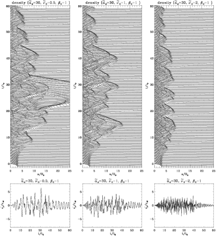
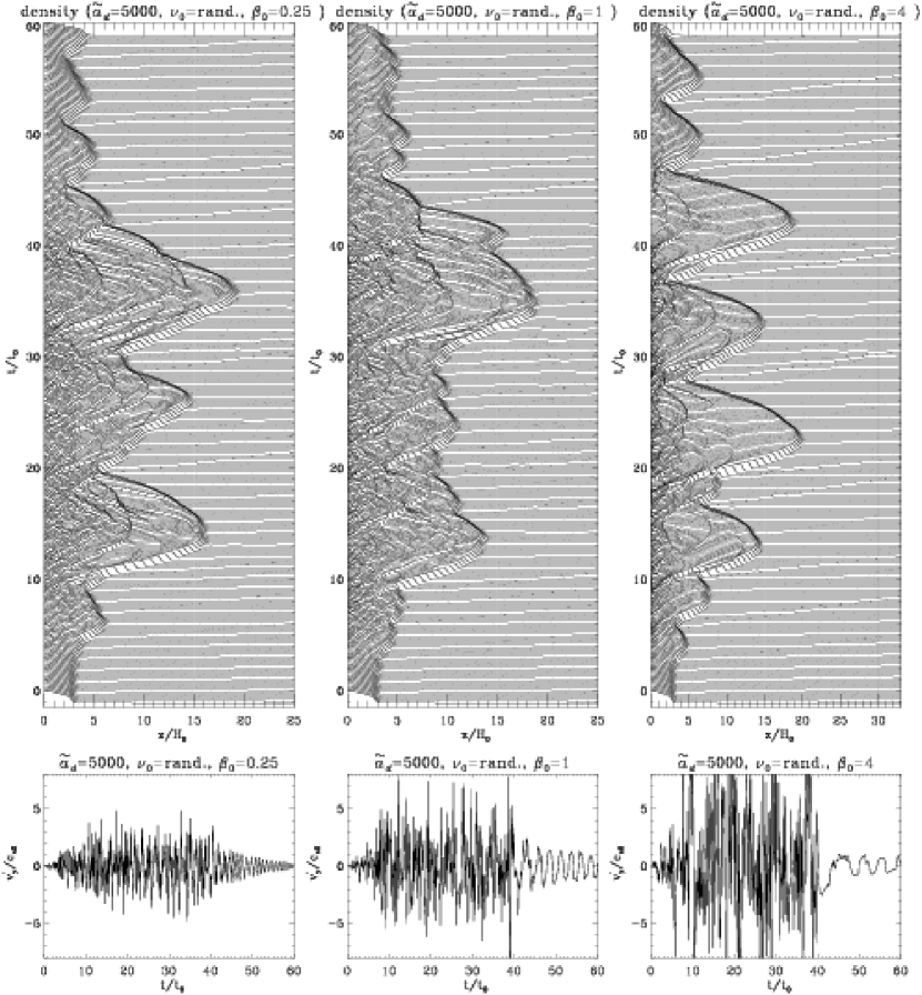
Figure 1 shows the time evolution of models with different frequencies $\tilde{\nu}_{0}$. The left panel shows the model with $\tilde{\nu}_{0}=0.5$, the middle panel shows the model with $\tilde{\nu}_{0}=1$, and the right panel shows the model with $\tilde{\nu}_{0}=2$; all models have $\tilde{a}_{d}=30$ and $\beta_{0}=1$. For each model, the upper panels show the time evolution of the density. The density profile at various times are stacked with time increasing upward in uniform increments of $0.2t_{0}$. The lower panels show the time evolution of $v^{\prime}_{y}$ at $z=0$, where $v^{\prime}_{y}$ is the oscillating component of the $y$-velocity that we defined in the previous section. As we have shown in Paper I, each density evolution plot shows many shock waves propagating in the cloud and significant upward and downward motions of the outer portion of the cloud during the period of constant energy input ($t=10t_{0}-40t_{0}$). Figure 1 shows that the cloud undergoes more expansion and the amplitude of $v^{\prime}_{y}$ becomes greater when the frequency is lower. We return to this point after examining the effect of $\beta_{0}$.

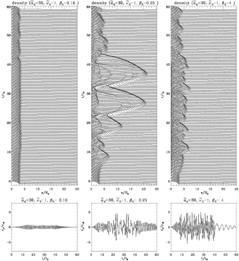
Figure 2 presents the same physical quantities as Figure 1, but for models with different values of $\beta_{0}$. The left panel shows the model with $\beta_{0}=0.16$, the middle panel shows the model with $\beta_{0}=0.25$, and the right panel shows the model with $\beta_{0}=4$; all models have $\tilde{a}_{d}=30$ and $\tilde{\nu}_{0}=1$. When $\beta_{0}=0.16$, the cloud hardly expands, showing no shock waves or large up-down motions. The velocity amplitude $v^{\prime}_{y}$ at $z=0$ is quite small in comparison to other models, and typically subsonic. This model has the strongest magnetic field for a given density, and corresponds to the most magnetically subcritical case. When $\beta_{0}=0.25$, the cloud shows large oscillations, although there are not as many shock waves as in the standard model with $\beta_{0}=1$ (middle panel of Fig. 1). The case of $\beta_{0}=4$ shows the greatest velocity amplitude $v^{\prime}_{y}$ at the midplane, and many shock waves. This is consistent with the trend set by other models that a weaker magnetic field leads to greater disturbances at the midplane for a given driving amplitude $\tilde{a}_{d}$. The $\beta_{0}=4$ model is significantly magnetically supercritical ($\mu_{\rm S}=2$). However, in contrast to the trend established for increasing $\beta_{0}$ by the other models, the cloud does not expand nearly as much as in the $\beta_{0}=0.25$ or $\beta_{0}=1$ models.

The differences in the level of cloud expansion for the models with differing $\tilde{\nu}_{0}$ and/or $\beta_{0}$ can be understood in part by considering the different wavelengths of the input driving. The input wavelength $\lambda_{0}$ is estimated from the Alfvén velocity at the midplane $V_{A0}$ and the period $T_{0}$ of the driving force:

$$\lambda_{0}\approx V_{A0}T_{0}=\frac{B_{0}}{\sqrt{4\pi\rho_{0}}}\frac{1}{\nu_{0}}=\frac{\sqrt{2}H_{0}}{\tilde{\nu}_{0}\sqrt{\beta_{0}}}\ .$$ (31)

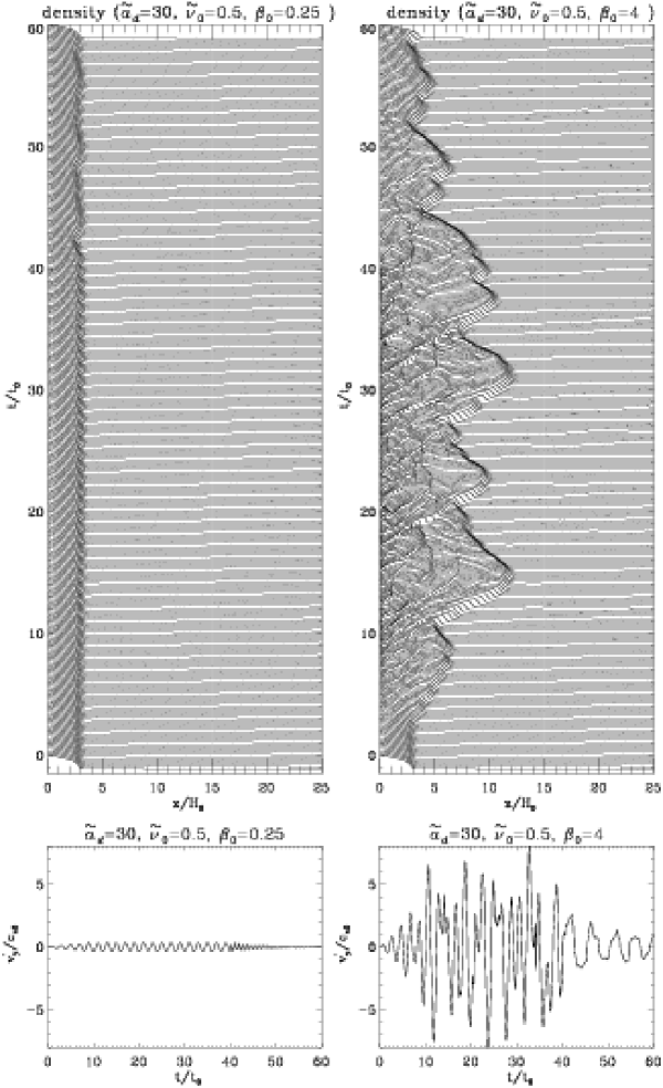
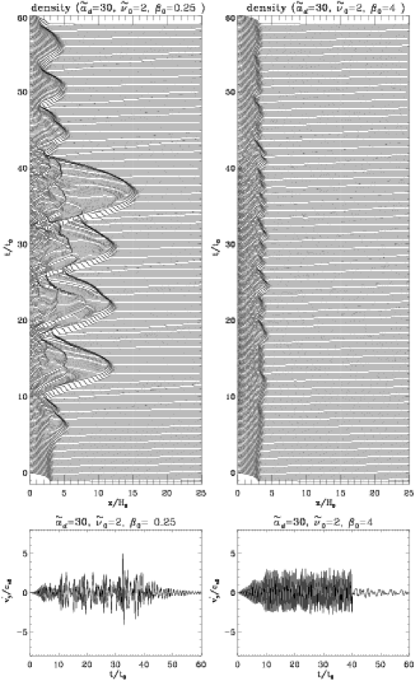
For the models presented in Figure 1 with $\tilde{\nu}_{0}=0.5,1,2$, the corresponding input wavelengths are $\lambda_{0}=2.83H_{0},1.41H_{0},0.71H_{0}$, respectively. The model with $\tilde{\nu}_{0}=0.5$ has an input wavelength closest to that of the initial cloud size ($\approx 3.0H_{0}$), and this leads to the greatest effect of cloud expansion due to the pressure of the nonlinear waves. This correlation is borne out further by examining the models of different $\beta_{0}$ presented in Figure 2. When $\beta_{0}=0.16$ and $\tilde{\nu}_{0}=1$, in addition to the low amplitude fluctuations $v^{\prime}_{y}$ due to the very strong magnetic field, we also have $\lambda_{0}\approx 3.5H_{0}$, which is larger than the initial cloud size. Hence, the waves are not effective at providing an internal pressure. When $\beta_{0}=0.25$ and $\tilde{\nu}_{0}=1$ we find $\lambda_{0}\approx 2.83H_{0}$, which is approximately the same as the initial cloud size. On the other hand, when $\beta_{0}=4$ and $\tilde{\nu}_{0}=1$ we get $\lambda_{0}\approx 0.71H_{0}$, which is significantly smaller than the cloud size. Even though there are large velocity fluctuations $v^{\prime}_{y}$ at the midplane in this model due to the relatively weak magnetic field, the overall expansion of the cloud is inhibited by the relatively small ratio $\lambda_{0}/H_{0}$. Our overall results indicate that the cloud suffers less expansion when the driving wavelength is larger than the initial cloud size, and the cloud is lifted up the most when the driving wavelength is approximately the same as the initial cloud size.

Figure 3 and Figure 4 show other models which differ from the standard model in the values of two separate parameters. The left panel of Figure 3 shows the model with $\beta_{0}=0.25$ and $\tilde{\nu}_{0}=0.5$, while the right panel shows the model with $\beta_{0}=4$ and $\tilde{\nu}_{0}=0.5$; both models have $\tilde{a}_{d}=30$. The driving wavelength $\lambda_{0}\approx 5.66H_{0}$ for the model in the left panel, and $\lambda_{0}\approx 1.41H_{0}$ for the model in the right panel. These two panels are the low frequency counterparts of the middle and right panels of Figure 2, respectively. Figure 3 also shows that the cloud suffers a lesser expansion when the driving wavelength is larger than the cloud size.

The left panel of Figure 4 shows the model with $\beta_{0}=0.25$ and $\tilde{\nu}_{0}=2$, and the right panel shows the model with $\beta_{0}=4$ and $\tilde{\nu}_{0}=2$; both models have $\tilde{a}_{d}=30$. The driving wavelength is $\lambda_{0}\approx 2.83H_{0}$ for the model in the left panel, and $\lambda_{0}\approx 0.354H_{0}$ for the model in the right panel. These two models are the high frequency counterparts of the models in Figure 3. In contrast to Figure 3, the model with $\beta_{0}=0.25$ shows greater expansion because the wavelength is comparable to the initial cloud size, while the model with $\beta_{0}=4$ shows very little expansion since the driving wavelength is much smaller than than the initial cloud size.

In Figure 5, we show the results of the models with a random driving force. The models have different values of $\beta_{0}$ and the same dimensionless amplitude $\tilde{a}_{d}=5000$. Since the random driving contains various frequencies, the time evolution of the density is not significantly different from model to model. Each model has a component of the driving at the wavelength (which is a function of $\beta_{0}$) that is comparable to the cloud size. However, the amplitudes of $v^{\prime}_{y}$ are a little different in each model. When the magnetic field is strong ($\beta_{0}=0.25$), the amplitude is smaller, and vice versa. This result is consistent with the results presented in Figure 2.

To conclude this section, we reemphasize that the wavelength of the driving force is an important parameter for the cloud evolution. The driving wavelength which is comparable to the cloud size has the greatest effect in expanding the cloud. Thus, the expansion cannot be attributed primarily to the commonly used notion of “turbulent pressure”, which requires that the wavelength of disturbances be much smaller than the typical scale length of the cloud (see Bonnazola et al. 1992; Martin, Heyvaerts, & Priest 1998).

3.2 Energy Dissipation Rate

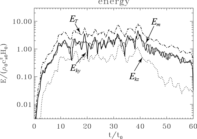
Figure 6 shows the time evolution of energies in the cloud for the case of random driving, $\tilde{a}_{d}=5000$ and $\beta_{0}=1$. Each energy is calculated in the following manner: kinetic energy of the $z$-component of velocity,

$$E_{kz}(t)=\int_{0}^{z_{f}(t)}\frac{1}{2}\rho v_{z}^{2}\,dz;$$ (32)

kinetic energy of the $y$-component of velocity,

$$E_{ky}(t)=\int_{0}^{z_{f}(t)}\frac{1}{2}\rho v_{y}^{2}\,dz-\,E_{km},$$ (33)

where $E_{km}$ is the kinetic energy of the mean motion of the cloud, i.e.,

$$E_{km}(t)=\frac{1}{2}\langle v_{m}\rangle^{2}\int_{0}^{z_{f}(t)}\rho\,dz;$$ (34)

magnetic energy of the $y$-component of the magnetic field,

$$E_{m}(t)=\int_{0}^{z_{f}(t)}\frac{B_{y}^{2}}{8\pi}\,dz;$$ (35)

the sum of the above terms,

$$E_{T}(t)=E_{kz}(t)+E_{ky}(t)+E_{m}(t).$$ (36)

In the above equations, the integration was done from 0 to $z_{f}(t)$ because we are interested in the energies of the cold material. Strictly speaking, the total energy in each case is twice the value we calculate due to the mirror symmetric boundary condition at $z=0$. Equation (33) shows that the mean kinetic energy of the cloud is subtracted from the kinetic energy of the the $y$-component of the velocity, so that $E_{ky}$ is the kinetic energy of the oscillatory motions.

In Figure 6, we examine the evolution of various energies for the random driving force model with $\tilde{a}_{d}=5000$ and $\beta_{0}=1$. The thick solid line shows $E_{ky}$, the thin solid line shows $E_{m}$, the dotted line shows $E_{kz}$, and the dashed-dotted line shows $E_{T}$. The values of each energy are smoothed out over a time $t=t_{0}$ to remove small oscillations. Figure 6 is similar to the Figure 8 in Paper I, which shows the evolution of these quantities in the standard model with sinusoidal driving force. Among the energies, $E_{ky}$ and $E_{m}$ are comparable to each other, but $E_{kz}$ is significantly smaller, i.e., there is approximate equipartition in transverse kinetic energy and magnetic fields, and there is much less energy in longitudinal modes. Longitudinal modes can be generated by the gradient of magnetic field pressure in the $z$-direction. However, the dominance of the transverse modes implies that the primary dissipation mechanisms are the nonlinear cascade and nonlinear steepening effects that transfer energy to progressively smaller scales until it is dissipated at the grid scale (see more extensive discussion in Paper I). After the driving force is terminated at $t=40t_{0}$, the energies decrease almost exponentially. The $e$-folding time is $t_{d}\simeq 10t_{0}$, which is approximately a sound crossing time across the cloud size as expanded by the turbulent pressure. The turbulent energy is nearly completely dissipated within a few of these crossing times. All of this is consistent with the results for sinusoidal driving presented in Paper I.

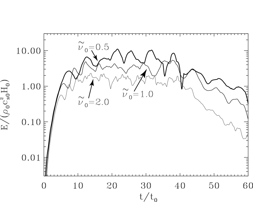
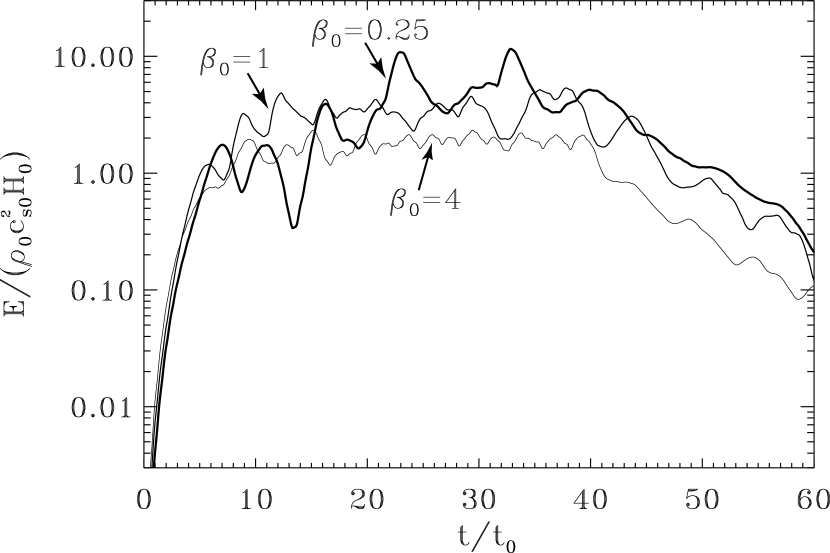
Figure 7 shows the time evolution of $E_{T}$ for different values of $\tilde{\nu}_{0}$ with fixed values of $\beta_{0}=1$ and $\tilde{a}_{d}=30$. Figure 8 also shows the time evolution of $E_{T}$ for different values for $\beta_{0}$ but with fixed values $\tilde{\nu}_{0}=1$ and $\tilde{a}_{d}=30$. The energy decreasing time appears to be somewhat lesser when the driving frequency is higher. The $e$-folding time of dissipation for each parameter is listed in Table 1. It appears to have a weak correlation with the cloud size. The smallest $e$-folding times ($t_{d}<4.0t_{0}$) occur when the wave length $\lambda_{0}$ is larger than the initial cloud size $\sim 3H_{0}$. In this case, most of the input energy escapes from the cloud without affecting it much. Overall, our results show that $t_{d}\approx 10t_{0}$ is a good approximation for most clouds, i.e., that $t_{d}$ does not depend very sensitively on most parameters.

3.3 Spatial Power Spectrum

Figure 9 shows the spatial power spectra of $B_{y}$ and $v_{y}$ for a model with $\tilde{a}_{d}=30$, $\tilde{\nu}_{0}=1$, and $\beta_{0}=1$. Both are plotted against the dimensionless quantity $kH_{0}$, where $k=1/\ell$ and $\ell$ is a length scale in the $z$-direction. The power spectra were taken at $t=30t_{0}$, in the midst of the period of steady turbulent driving, over the spatial range $z=0-60H_{0}$. There is a weak indication of a local peak in the power spectrum of $B_{y}$ around $k=1/\lambda_{0}\approx 0.70/H_{0}$, which corresponds to the driving scale $\lambda_{0}\approx 1.41H_{0}$. However, the main result here is that there is significant power on scales larger than the driving scale ($k<0.70/H_{0}$) in the spectra of both $B_{y}$ and $v_{y}$. The dotted line shows the dependence $k^{-5/3}$ for comparison; it is the Kolomogorov power spectrum for one-dimensional incompressible hydrodynamic motions (e.g., Elmegreen & Scalo 2004). Our simulations of compressible MHD motions shows both spectra are similar but have slightly steeper than $k^{-5/3}$ slopes on small scales($k>H_{0}^{-1}$). Figure 10 shows the same power spectra for the random perturbation model with $\tilde{a}_{d}=1000$, and $\beta_{0}=1$. These power spectra confirm the basic result of the sinusoidal models that there is significant power on large scales ($k<H_{0}^{-1}$) and that the slopes are steeper than $k^{-5/3}$ on small scales($k>H_{0}^{-1}$).

The power spectra show that there is significant power on the largest scales in the cloud and that the power spectrum naturally evolves to the form $k^{-p}$, where $p$ is a positive number, even if driving occurs within the cloud on a sub-cloud scale. This large-scale power comes from the wave propagation in the gravitationally stratified cloud. When a wave propagates into the low density region with greater Alfvén speed, the wavelength becomes larger. The waves of larger wavelengths also generally have less dissipation. These principles lead to significant power on larger scales in a gravitationally stratified cloud.

3.4 Correlations between Velocities and Sizes

Figure 11 plots the time averaged velocity dispersions $\langle\sigma^{2}\rangle_{t}^{1/2}$ of Lagrangian fluid elements within various model clouds as a function of $\langle z\rangle_{t}$, where

$$\sigma=\sqrt{\text@frac{1}{2}[v_{z}^{2}+(v^{\prime}_{y})^{2}]+c_{s}^{2}},$$ (37)

and $\langle z\rangle_{t}$ is the time-averaged height of each Lagrangian fluid element. The open circles ($\sigma_{F}$, $z_{F}$ in Table 1) correspond to Lagrangian fluid elements whose initial positions are located at $z=2.51H_{0}$, which is close to the edge of the cold cloud. The filled circles ($\sigma_{H}$, $z_{H}$ in Table 1) correspond to Lagrangian fluid elements whose initial positions are located at $z=0.61H_{0}$, which is approximately the half-mass position of the cold cloud. An open and filled circle is plotted for each model in our complete parameter study; some basic properties of each model are summarized in Table 1. The dotted line shows

$$\langle\sigma^{2}\rangle_{t}^{1/2}\propto\langle z\rangle_{t}^{0.5}.$$ (38)

This figure shows that the model clouds are in a time-averaged self-gravitational equilibrium state under the influence of turbulent pressure (see Paper I). The varying parameters can affect the position of the circles, but all model clouds obey the basic correlation shown by the dotted line. This is consistent with the observational line-width–size relation of molecular clouds (Larson 1981; Myers 1983; Solomon et al. 1987).

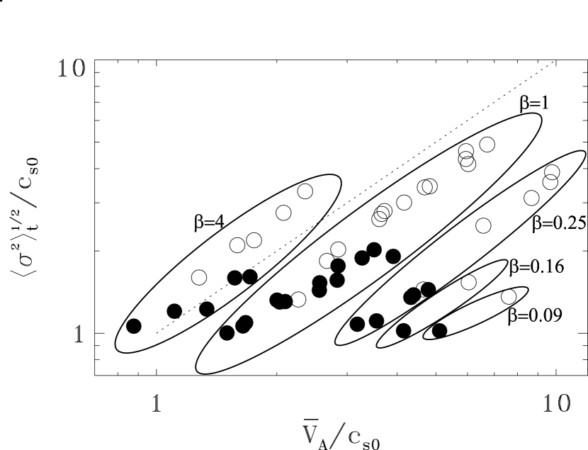
Figure 12 shows the correlation between the velocity dispersion and mean Alfvén velocity of the cloud $\bar{V}_{A}$ at the mean position $\langle z\rangle_{t}$ of the Lagrangian elements. The mean Alfvén velocity is defined by

$$\bar{V}_{A}\equiv\frac{B_{0}}{\sqrt{4\pi\bar{\rho}}},$$ (39)

where

$$\bar{\rho}=\frac{\Sigma}{2\langle z\rangle_{t}}$$ (40)

is the mean density and $\Sigma$ is the column density for each Lagrangian element. The dotted line shows

$$\langle\sigma^{2}\rangle_{t}^{1/2}\propto\bar{V}_{A}.$$ (41)

Results from model clouds with the same $\beta_{0}$ are circled and marked. They show that the velocity dispersions have a good correlation with the mean Alfvén velocity if each cloud has a similar value of $\beta_{0}$, i.e. mass-to-flux ratio. An analysis of the magnetic field measurements compiled by Crutcher (1999) shows that there is an excellent correlation between the line-of-sight component of the large-scale magnetic field $B_{\rm los}$ and $\sigma\rho^{1/2}$ for observed clouds of widely varying values of $\rho$, $B_{\rm los}$, and $\sigma$ (Basu 2000). This is essentially the same correlation as equation (41); the observational data actually imply an average value $\sigma/\bar{V}_{A}\approx 0.5$ (see Basu 2005 for discussion). Our models are consistent with this ratio if $\beta_{0}\approx 1$, i.e the mass-to-flux ratio is essentially equal to the critical value. A comparison of observed values of $B_{\rm los}$ and column density also reveals that the mass-to-flux ratios are always very close to the critical value (Crutcher 1999; Shu et al. 1999; Crutcher 2004; Basu 2005).

4 Summary and Discussion

We have performed 1.5-dimensional numerical simulations of nonlinear MHD waves in a gravitationally stratified molecular cloud that is bounded by a hot and tenuous external medium. Using the same basic model as presented in Paper I (Kudoh & Basu 2003), we have carried out a parameter survey by varying the frequency of the driving force and the magnetic field strength of the cloud. We found that the key parameter for the evolution of the cloud is the Alfvén wavelength of the driving force. If the wavelength is larger than the size of the cloud, the cloud is affected less by the waves. The wavelength that is the same order of the cloud size is the most effective in expanding the cloud. This means that turbulent expansion is different than the usual notion of expansion due to a “turbulent pressure” in which the wavelengths need to be much smaller than the cloud size. We also studied the effect of a driving force that varies randomly with time and found that significant cloud expansion occurs since there is always a component of the driving that is at a favorable frequency for expanding the cloud. The evolution of our model clouds reveal the following general features: (1) Under the influence of a driving source of Alfvénic disturbances, a cloud shows significant upward and downward motions, with an oscillation time scale that is comparable to the cloud crossing time; (2) After driving is discontinued, the turbulent energy dissipates exponentially with time, with an $e$-folding time essentially equal to the crossing time across the expanded cloud rather than the crossing time of the driving scale; (3) The power spectra show that significant power is generated on scales larger than that of the turbulent driving ($k<H_{0}^{-1}$); (4) The line-width–size relation is obtained by an ensemble of clouds with different physical parameters which are individually in a time-averaged self-gravitational equilibrium state. The largest amplitude random motions occur in the outer low density regions of a stratified cloud. The magnetic field data is best fit by models with $\beta_{0}\approx 1$, which implies that the mass-to-flux ratio is very close to the critical value for collapse.

In the case of the random driving force, we require a much larger driving amplitude $\tilde{a}_{d}$ than for the sinusoidal case in order to get a comparable expansion of the cloud (see Table 1). This is due to the multiplication by a random number in the range $[-1,1]$ at each time step (see eq. [21]) in the random case. The resulting driving efficiency is quite low since the driving force $F(z,t)$ is often out of phase with $v_{y}$, resulting in a lesser amount of work done in the random case than in the sinusoidal case for a given value of $\tilde{a}_{d}$. A physically meaningful comparison of the energetics of the random and sinusoidal cases can be done by calculating the energy flux of Alfvén waves emerging from just outside the region of the artificial driving. We define the Alfvén energy flux in the $z$-direction to be

$${\cal F}_{A}=-\frac{B_{z}B_{y}}{4\pi}(v_{y}-\langle v_{m}\rangle),$$ (42)

and perform the calculation at $z=z_{a}=0.1H_{0}$. We find that the time-averaged energy flux of a random driving model with parameters $\tilde{a}_{d}=5000$ and $\beta_{0}=1$ is comparable to (actually about twice as large as) that of a sinusoidal driving model with parameters $\tilde{a}_{d}=30$, $\beta_{0}=1$, and $\nu_{0}=1$.

For the random driving case ($\tilde{a}_{d}=5000$, $\beta_{0}=1$), the time-averaged energy flux measured near the surface of the cloud (at the full-mass position) is about 20% of that at $z=z_{a}$, so that about 80% of the input energy is dissipated in the cloud. For the sinusoidal driving case ($\tilde{a}_{d}=30$, $\beta_{0}=1$, $\nu_{0}=1$), the energy flux near the surface is about 30% of that at $z=z_{a}$. The small difference may arise because the random model contains many high frequency waves which dissipate quickly. In each case, the dissipated energy flux measured while the driving term is applied is comparable to $E_{T}/t_{d}$, where $E_{T}$ is the steady-state value of the sum of fluctuating magnetic and kinetic energies during the turbulent driving phase, and $t_{d}$ is the dissipation time measured after turbulent driving is discontinued. Our obtained value $t_{d}\simeq 10t_{0}$, which does not depend sensitively on most parameters, is somewhat longer than that estimated from three-dimensional periodic box simulations. We believe that part of the discrepancy comes from the generation of longer wavelength modes as the waves travel to low-density regions near the cloud’s surface. However, one-dimensional simulations are also known to have lower dissipation rates than two- or three-dimensional ones (Ostriker et al. 2001). Therefore, higher dimensional simulations that include density-stratification of the cloud will give the final answer in the future.

In our ideal MHD model there is no wave damping due to ion-neutral friction, although there is wave damping due to a nonlinear cascade and nonlinear steepening, as well as leakage of wave energy into the external medium (see Paper I for a more extensive discussion). We expect that ion-neutral friction would be most effective at damping the shortest wavelength modes in our simulation (Kulsrud & Pearce 1969), and that the power spectra of $B_{y}$ and $v_{y}$ may become steeper at high wavenumber. However, our current results show that the wavelengths that are comparable to the initial cloud size are most effective at expanding the cloud, so it is not clear exactly how effective ion-neutral friction would be in removing turbulent cloud support. Furthermore, we are modeling the large scale evolution of molecular clouds with mean column densities of up to a few times 10${}^{21}\,~{}{\rm cm}^{-2}$, or visual extinction $A_{V}\lesssim 3$. At these column densities, the clouds are expected to be significantly ionized by background far-ultraviolet starlight so that ion-neutral friction will take a prohibitively long time (McKee 1989). Our results show that the dense midplane of the cloud has transonic or subsonic motions, and we expect these regions to decouple from the more turbulent low density envelope and develop higher column density regions in which the far-ultraviolet background is shielded (McKee 1989). In these regions, the ionization fraction is significantly lesser, and ambipolar diffusion can enhance the process of core formation. Therefore, models of fragmentation of a thin-layer which include the effects of magnetic fields and partial ionization due to cosmic rays (Basu & Ciolek 2004) form a complementary approach to ours.

Our model has the advantage of being global by virtue of including the effect of cloud stratification and a cloud boundary, rather than being a local periodic box model. The 1.5-dimensional approximation has also allowed extremely high resolution which can more accurately track the propagation of MHD waves. Our localized turbulent driving source is an artificial construct that mimics the various possible sources of disturbances in a real cloud. However, a general result is that the wave energy gets quickly redistributed throughout the cloud in such a way that most of the energy is on the largest scales. This result provides a way out of the “luminosity problem” posed by Basu & Murali (2001), since the dissipation rate is then set by the crossing time of the cloud scale rather than that of the internal driving scale. Our modeled clouds have a steady-state size $\sim 1$ pc and large-scale velocity dispersion $\sim 1~{}\rm km~{}s^{-1}$, which makes them comparable to observed dark clouds which can form groupings known as the giant molecular clouds (GMC’s; see e.g., Blitz & Williams 1999). The turbulent dissipation typically occurs with an $e$-folding time of a few Myr and is completely dissipated by $\sim 10^{7}$ yr. Even in the case that real molecular clouds and GMC’s start their life in a turbulent state and then evolve with no further external turbulent input, our results show that the turbulent lifetime is less than but within reach of estimated GMC lifetimes, $\sim 10^{7}$ yr; see discussion in Larson (2003). This provides another important motivation for future global three-dimensional models which can follow the actual sources of internal turbulent driving. As turbulence initially dissipates and a cloud contracts, we expect a transformation of some released gravitational potential energy back into MHD wave energy. In addition, much of the internal driving may be attributable to the outflows commonly launched from the near environs of protostars (see e.g., Bachiller & Tafalla 1999).

$\tilde{a}_{d}$	$\beta_{0}$	$\tilde{\nu}_{0}$	$\lambda_{0}/H_{0}$	$\langle z_{F}\rangle_{t}/H_{0}$	$\langle\sigma_{F}^{2}\rangle_{t}^{1/2}/c_{s0}$	$\langle z_{H}\rangle_{t}/H_{0}$	$\langle\sigma_{H}^{2}\rangle_{t}^{1/2}/c_{s0}$	$t_{d}/t_{0}$
10	1	1	1.41	4.00	2.03	0.760	1.09	9.0
20	1	1	1.41	6.82	2.80	1.13	1.30	5.5
30	1	1	1.41	10.8	3.42	1.78	1.53	8.5
40	1	1	1.41	17.9	4.16	2.91	1.88	9.0
50	1	1	1.41	17.4	4.34	3.34	2.02	15.0
30	1	2	0.707	6.42	2.62	1.20	1.31	6.0
50	1	2	0.707	8.54	3.01	1.78	1.44	5.5
30	1	0.5	2.83	17.4	4.63	2.20	1.76	9.5
20	1	0.5	2.83	6.60	2.73	1.09	1.32	6.5
30	0.09	1	4.71	2.57	1.36	0.639	1.02	2.5
30	0.16	1	3.54	2.88	1.54	0.750	1.02	3.0
30	0.25	1	2.83	11.5	3.57	1.32	1.38	9.0
20	0.25	1	2.83	5.33	2.47	0.86	1.11	8.0
30	4	1	0.707	5.00	2.10	1.34	1.20	8.0
50	4	1	0.707	6.06	2.19	1.94	1.23	8.0
30	0.25	2	2.83	9.28	3.12	1.28	1.35	8.0
30	4	2	0.354	3.22	1.60	0.837	1.06	8.0
30	0.25	0.5	5.66	2.67	1.45	0.688	1.08	4.0
30	4	0.5	1.41	8.52	2.76	2.68	1.59	8.5
5000	1	random	–	11.5	3.45	2.18	1.56	9.0
5000	0.25	random	–	11.8	3.88	1.56	1.44	6.5
5000	4	random	–	10.9	3.31	3.20	1.61	7.5
10000	1	random	–	22.3	4.90	4.16	1.91	7.5
1000	1	random	–	3.51	1.84	0.736	1.06	7.5
100	1	random	–	2.53	1.33	0.612	1.00	6.5

Figure 1: The time evolution for different frequencies ($\tilde{\nu}_{0}=0.5$, $\tilde{\nu}_{0}=1$, $\tilde{\nu}_{0}=2$) with the same parameters of $\tilde{a}_{d}=30$ and $\beta_{0}=1$. The upper panels show the time evolution of density. The density profile at various times are stacked with time increasing upward in uniform increments of $0.2t_{0}$. The lower panels show the time evolution of $v^{\prime}_{y}$ at $z=0$.

Figure 2: The same as Figure 1 but for different plasma beta ($\beta_{0}=0.16$, $\beta_{0}=0.25$, $\beta_{0}=4$) with the same $\tilde{a}_{d}=30$ and $\tilde{\nu}_{0}=1$.

Figure 3: The same as Figure 1 but for different parameters. The left panel shows the case of $\beta_{0}=0.25$, $\tilde{\nu}_{0}=0.5$ and $\tilde{a}_{d}=30$. The right panel shows the $\beta_{0}=4$, $\tilde{\nu}_{0}=0.5$ and $\tilde{a}_{d}=30$.

Figure 4: The same as Figure 1 but for different parameters. The left panel shows the case of $\beta_{0}=0.25$, $\tilde{\nu}_{0}=4$ and $\tilde{a}_{d}=30$. The right panel shows the $\beta_{0}=4$, $\tilde{\nu}_{0}=2$ and $\tilde{a}_{d}=30$.

Figure 5: The time evolution for random driving case with $\tilde{a}_{d}=5000$. The left panel shows the case of $\beta_{0}=0.25$, the middle panel shows $\beta_{0}=2$, and the right panel shows $\beta_{0}=4$.

Figure 6: Time evolution of various energies in the cloud for random driving force with $\tilde{a}_{d}=5000$ and $\beta_{0}=1$. The thick solid line shows $E_{ky}$, the dotted line shows $E_{kz}$, the thin solid line shows $E_{m}$, and dash-dotted line shows $E_{T}=E_{ky}+E_{kz}+E_{m}$. The values of each energy are smoothed out over a time $t_{0}$ in order to remove small oscillations originating from the driving force.

Figure 7: Time evolution of $E_{T}=E_{ky}+E_{kz}+E_{m}$ in the cloud for different frequencies ($\tilde{\nu}_{0}=0.5$, $\tilde{\nu}_{0}=1$, $\tilde{\nu}_{0}=2$) with the same parameters of $\tilde{a}_{d}=30$ and $\beta_{0}=1$. The thick solid line shows the case of $\tilde{\nu}_{0}=0.5$, the solid line shows $\tilde{\nu}_{0}=1$, and the thin solid line shows $\tilde{\nu}_{0}=2$. The values of each energy are smoothed out over every one cycle of the driving force in order to remove small oscillations originating from the driving force.

Figure 8: Time evolution of total energies in the cloud for different plasma beta ($\beta_{0}=0.25$, $\beta_{0}=1$, $\beta_{0}=4$) with the same parameters of $\tilde{a}_{d}=30$ and $\tilde{\nu}_{0}=1$. The thick solid line shows the case of $\beta_{0}=0.25$, the solid line shows $\beta_{0}=1$, and the thin solid line shows $\beta_{0}=4$. The values of each energy are smoothed out over every one cycle of the driving force in order to remove small oscillations originating from the driving force.

Figure 9: Spatial power spectra of $B_{y}$ and $v_{y}$ for the case of the sinusoidal driving force with parameters $\tilde{a}_{d}=30$, $\tilde{\nu}_{0}=1$ and $\beta_{0}=1$. The spectra were taken from a snapshot at $t=30t_{0}$. The dotted line is proportional to $k^{-5/3}$ and is shown for comparison.

Figure 10: Spatial power spectra of $B_{y}$ and $v_{y}$ for the case of the random driving force with parameters $\tilde{a}_{d}=5000$ and $\beta_{0}=1$. The spectra were taken from the snapshot at $t=30t_{0}$. The dotted line is proportional to $k^{-5/3}$ and is shown for comparison.

Figure 11: Time averaged velocity dispersions of different Lagrangian fluid elements for different parameters as a function of time averaged positions. The open circles correspond to Lagrangian fluid elements whose initial positions are located at $z=2.51H_{0}$, which is close to the edge of the cold cloud. The filled circles correspond to Lagrangian fluid elements whose initial positions are located at $z=0.61H_{0}$, which is approximately the half-mass position of the cold cloud. The dotted line shows $\langle\sigma^{2}\rangle_{t}^{1/2}\propto\langle z\rangle_{t}^{0.5}$. Each circle can be associated with a particular model in our study by comparison with the numbers in Table 1.

Figure 12: Time averaged velocity dispersions as a function of the mean Alfvén velocity of the cloud. The results from the same plasma beta are encircled. The open circles correspond to Lagrangian fluid elements whose initial positions are located at $z=2.51H_{0}$. The filled circles correspond to Lagrangian fluid elements whose initial positions are located at $z=0.61H_{0}$. The dotted line shows $\langle\sigma^{2}\rangle_{t}^{1/2}\propto\bar{V}_{A}$.

References

- (1) Bachiller, R., & Tafalla, M. 1999, in The Origin of Stars and Planetary Systems, ed. C. J. Lada & N. Kylafis (Dordrecht: Kluwer), 227
- (2) Basu, S. 2000, ApJ, 540, L103
- (3) Basu, S. 2005, in Young Local Universe, Proceedings of XXXIXth Rencontres de Moriond, eds. A. Chalabaev, T. Fukui, T. Montmerle, and J. Tran-Thanh-Van, (Editions Frontières, Paris)
- (4) Basu, S., & Ciolek, G. E. 2004, ApJ, 607, L39
- (5) Basu, S., & Murali, C. 2001, ApJ, 551, 743
- (6) Blitz, L., & Williams, J. P. 1999, in The Origin of Stars and Planetary Systems, ed. C. J. Lada & N. Kylafis (Dordrecht: Kluwer), 3
- (7) Bonazzola, S., Perault, M., Puget, J. L., Heyvaerts, J., Falgarone, E., & Panis, J. F. 1992, J. Fluid Mech., 245, 1
- (8) Brunt, C. M., & Heyer, M. H. 2002, ApJ, 566, 276
- (9) Cho, J., & Lazarian, A. 2003, MNRAS, 345, 325
- (10) Cho, J., Lazarian, A., & Vishniac, E. T. 2002, ApJ, 564, 291
- (11) Crutcher, R. M. 1999, ApJ, 520, 706
- (12) Crutcher, R. M. 2004, Ap&SS, 292, 225
- (13) Folini, D., Heyvaerts, J., & Waleder, R. 2004, A&A, 414, 559
- (14) Elmegreen, B. G., & Scalo J. 2004, ARA&A, 42, 211
- (15) Goldsmith, P. F., & Langer, W. D. 1978, ApJ, 222, 881
- (16) Hartmann, L. 2002, ApJ, 578, 914
- (17) Houde, M. Dowell, C. D., Hildebrand, R. H., Dotson, J. L., Vaillancourt, J. E., Phillips, T. G., Peng, R., & Bastien, P. 2004, ApJ, 604, 717
- (18) Kudoh, T., & Basu. S. 2003, ApJ, 595, 842
- (19) Kudoh, T., Matsumoto, R., & Shibata, K. 1999, CFD J., 8, 56
- (20) Kulsrud, R., & Pearce, W. P. 1969, ApJ, 156, 445
- (21) Lada, C. J., Bergin, E. A., Alves, J. F., & Huard, T. L. 2003, ApJ, 586, 286
- (22) Larson, R. B. 1981, MNRAS, 194, 809
- (23) Larson, R. B. 2003, Rep. Prog. Phys., 66, 1651
- (24) Mac Low, M.-M. 1999, ApJ, 524, 169
- (25) Mac Low, M.-M., Klessen, R. S., Burkert, A., & Smith, M. D. 1998, Phys. Rev. Lett. 80, 2754
- (26) Martin, C. E., Heyvaerts, J., & Priest, E. R. 1997, A&A, 326, 1176
- (27) McKee, C. F. 1989, ApJ, 345, 782
- (28) McKee, C. F. 1999, in The Origin of Stars and Planetary Systems, ed. C. J. Lada & N. Kylafis (Dordrecht: Kluwer), 29
- (29) Matthews, B. C., & Wilson, C. D. 2000, ApJ, 531, 868
- (30) Mizuno, A., Onishi, T., Yonekura, Y., Nagahama, T., Ogawa, H., & Fukui, Y. 1995, ApJ, L161
- (31) Myers, P. C. 1983, ApJ, 270, 105
- (32) Myers, P. C. 2005, ApJ, 623, 280
- (33) Myers, P. C., & Goodman, A. A. 1988, ApJ, 326, L27
- (34) Onishi, T., Mizuno, A., Kawamura, A., Ogawa, H., & Fukui, Y. 1998, ApJ, 502, 296
- (35) Onishi, T., Mizuno, A., Kawamura, A., Tachihara, K., & Fukui, Y. 2002, ApJ, 575, 950
- Ostriker, Stone, & Gammie (2001) Ostriker, E. C., Stone, J. M., & Gammie, C. F. 2001, ApJ, 546, 980
- (37) Padoan, P., & Nordlund, A. P. 1999, ApJ, 526, 279
- (38) Schleuning, D. A. 1998, ApJ, 493, 811
- (39) Shu, F. H., Allen, A., Shang, H., Ostriker, E. C., & Li, Z.-Y. 1999, in The Origin of Stars and Planetary Systems, ed. C. J. Lada & N. Kylafis (Dordrecht: Kluwer), 193
- (40) Solomon, P. M., Rivolo, A. R., Barrett, J., & Yahil, A. 1987, ApJ, 319, 730
- (41) Spitzer, L., Jr. 1942, ApJ, 95, 329
- (42) Stone, J. M., Gammie, C. F., & Ostriker, E. C. 1998, ApJ, 508, L99
- (43) Stone, J. M., & Norman, M. L. 1992, ApJS, 80, 791
- (44) Sugimoto, K., Hanawa, T., & Fukuda, N. 2004, ApJ, 609, 810
- (45) Ungerechts, H., & Thaddeus, P. 1987, ApJS, 63, 645
- (46) Yabe, T., Xiao, F., & Utsumi, T. 2001, J. Comput. Phys., 169, 556