Location of the solar dynamo and near-surface shear

Abstract

The location of the solar dynamo is discussed in the context of new insights into the theory of nonlinear turbulent dynamos. It is argued that, from a dynamo-theoretic point of view, the bottom of the convection zone is not a likely location and that the solar dynamo may be distributed over the convection zone. The near surface shear layer produces not only east-west field alignment, but it also helps the dynamo disposing of its excess small scale magnetic helicity.

Nordita, Blegdamsvej 17, D-2100 Copenhagen Ø, Denmark

1. Introduction

It is commonly taken for granted that the solar dynamo has to work at the bottom of the convection zone, or that at least the toroidal field is generated or stored down there (Spiegel & Weiss 1980, Golub et al. 1981, Galloway & Weiss 1981, Choudhuri 1990). This expectation results mostly from the fact that only at the bottom of the convection zone the dynamical time scales associated with convection and magnetic buoyancy are long enough to be comparable with the rotational period. There is also the notion that the magnetic field needs to be ‘stored’ over a significant fraction of the solar cycle period and that this is only conceivable at or below the base of the convection zone. There are several other aspects in favor of placing the dynamo at the bottom of the convection zone. One is the large extent of the active regions (up to $100\,{\rm Mm}$) that is only compatible with length scales typical of the deep convection zone (Galloway & Weiss 1981). Another argument is that it is at the bottom of the convection zone that we have a strong radial shear layer where $r\partial\Omega/\partial r\neq 0$. However, there is of course also latitudinal differential rotation ($\partial\Omega/\partial\theta\neq 0$) that is actually stronger, and there is still extremely strong radial shear just beneath the surface in the uppermost $30\,{\rm Mm}$ of the Sun (see Fig. 1). So, we see that the shear argument is problematic. In addition, at the bottom of the convection zone the sign of the radial shear is such that standard dynamo theory would predict an equatorward migration only when the $\alpha$ effect is negative. Very near the bottom of the convection zone the $\alpha$ effect is indeed predicted to have the opposite sign according to the standard formalism (Krivodubskii 1984). However, there is a whole host of other problems. First of all, the radial shear seen at the bottom of the convection zone is strongest at the poles and this is also where $\alpha$ is strongest. So, in spite of spherical geometry factors the magnetic activity predicted by overshoot layer dynamos is far too strong at the poles and needs to be artificially suppressed if this approach is to be viable (Rüdiger & Brandenburg 1995, Markiel & Thomas 1999). Secondly, such overshoot layer dynamos (also sometimes called tachocline dynamos) have the well-known problem of producing too many toroidal field belts in the meridional plane (Moss et al. 1990). Furthermore, the negative radial angular velocity gradient in the bulk of the convection zone and especially at the bottom tends to produce the wrong migration direction of the magnetic activity, i.e. poleward rather than equatorward (Parker 1987). Although this problem could be fixed by invoking a strong negative value of $\alpha$ at the bottom of the convection zone, there remains always the problem with the phase relation between radial and azimuthal fields, i.e. $B_{r}B_{\phi}$ is observed to be negative, but it would be positive with positive radial shear (Yoshimura 1976, Stix 1976).

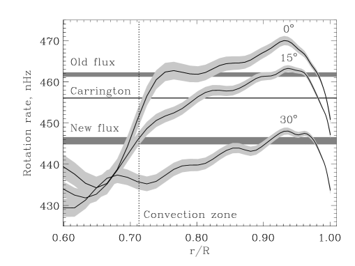
Figure 1.: Radial profiles of the internal solar rotation rate, as inferred from helioseismology. The rotation rate of active zones at the beginning of the cycle (at $\approx 30^{\circ}$ latitude) and near the end (at $\approx 4^{\circ}$) is indicated by horizontal bars, which intersect the profiles of rotation rate at $r/R_{\odot}\approx 0.97$. Courtesy of Benevolenskaya et al. (1999).

Even if one ignored all these problems, there are still a number of difficulties associated with the idea of having a dynamo operating at the bottom of the convection zone. Firstly, in order for the flux tubes to be correctly oriented after their ascent, the field strength of the flux tube has to be very strong ($\sim 100\,{\rm kG}$) to resist extraordinarily strong distortions and tilt. However, it is hard to imagine that the field strength exceeds the equipartition value ($\sim 1\,{\rm kG}$) by a factor of a hundred, and this has not yet been demonstrated. Secondly, it is hard to imagine that the flux tubes would not disrupt by expanding too much before forming a neat sunspot pair.

These are problems and difficulties that we have been living with for quite a few years when constructing overshoot layer dynamos. However, there is also the possibility of placing the dynamo right in the middle of the convection zone. This idea may appear rather uncomfortable at first, but to people working in dynamo theory it is a rather natural and appealing scenario. The basic picture is one where dynamo action occurs in the bulk of the convection zone, affected obviously by the near-surface shear layer. Downward pumping will also operate, so as to prevent the magnetic field from floating upwards on too short a time scale (Nordlund et al. 1992, Tobias et al. 1998). However, in this scenario the field that we observe as sunspots at the surface is likely to come from the near surface layers, where sunspots may form as a result of convective collapse of magnetic fibrils (Zwaan 1978, Spruit & Zweibel 1979), possibly facilitated by negative turbulent magnetic pressure effects (Kleeorin et al. 1996) or by an instability (Kitchatinov & Mazur 2000) causing the vertical flux to concentrate into a tube. The anticipated averaged field strength in the convection zone would be about $300\,{\rm G}$, i.e. about $10\%$ of the equipartition value. This field may then get amplified locally near the surface. In that sense, sunspots are not be deeply rooted, but rather a shallow phenomenon rooted at a depth of $20$–$30\,{\rm Mm}$.

2. Distributed dynamos with shear

In this section we discuss some of the properties of turbulent dynamos that are strongly affected by shear. Some of the recent findings have been presented in an earlier paper (Brandenburg 2005; hereafter B05). Here we will only review the main aspects. Before going into details, it is important to put this research into perspective. Let us distinguish three different aspects of dynamos. There are first of all the mean field dynamos, which is based on a theory for the averaged magnetic field, whose evolution is dominated by parameters such as $\alpha$ effect and turbulent diffusivity. Without any independent confirmation of the existence and magnitude of these coefficients, the predictive power of this approach is limited. We shall not be concerned with this approach in any details, except for the comparison with other approaches. Then there are dynamos where turbulence is not parameterized, but it is explicitly being solved for using computer simulations at the highest possible resolution. Two types of these dynamos can be distinguished: small scale and large scale dynamos. Both are turbulent and both have small scale magnetic fields, but the large scale dynamos also show large scale spatial coherence, and in some cases even long term temporal coherence such as magnetic cycles. The latter type of dynamo is clearly relevant to the Sun, while the former one may be dominant in many simulations.

A general remark is here in order. In many simulations the magnetic Prandtl number (ratio of viscosity to magnetic diffusivity) is of order unity, while in the Sun it is $<10^{-4}$. Only in recent years the possible significance has been clarified. It turns out that for progressively smaller magnetic Prandtl numbers the threshold for dynamo action moves to larger magnetic Reynolds numbers. In the paper by Haugen et al. (2004) it was found that, for a limited parameter range, the critical magnetic Reynolds numbers scales with the magnetic Prandtl number to the $-1/2$ power. However, in reality this dependence may actually not be a power law and there are now suggestions that the slope may become steeper toward smaller values of the magnetic Prandtl number, and that small scale dynamos may even become completely impossible below a certain critical value (Schekochihin et al. 2005). At the same time, the large scale dynamo is largely independent of magnetic Prandtl number, as will be discussed next.

A prime example of a large scale turbulent dynamo is in the presence of helicity. In this case the magnetic Reynolds number, defined here as $R_{\rm m}=u_{\rm rms}/(\eta k_{\rm f})$, where $u_{\rm rms}$ is the rms velocity, $\eta$ the magnetic diffusivity, and $k_{\rm f}$ the typical wavenumber where the kinetic energy spectrum peaks. Both for $P_{\rm m}=1$ and for $P_{\rm m}=0.1$ the critical value of $R_{\rm m}$ for large scale dynamo action is around unity [see Table 1 of Brandenburg (2001), but there the magnetic Reynolds numbers need to be divided by $2\pi$ to comply with the definition above]. If the absence of small scale dynamo action for small magnetic Prandtl numbers is confirmed, this might suggest that in bodies such as the Sun, only large scale dynamo action is possible, but not small scale dynamo action. Alternatively, the naive extrapolation to solar parameters may be invalid, so it is possible that for sufficiently small values of the magnetic Prandtl number the critical value of $R_{\rm m}$ for small scale dynamo action levels off at a constant value of perhaps several hundred (Boldyrev & Cattaneo 2004). However, such high values are currently still out of reach for direct simulations.

Figure 2.: Evolution of the energies of the total field $\langle{\bm{B}}^{2}\rangle$ and of the mean field $\langle\overline{\bm{B}}^{2}\rangle$, in units of $B_{\rm eq}^{2}$, for runs with non-helical forcing and open or closed boundaries; see the solid and dotted lines, respectively. The inset shows a comparison of the ratio $\langle\overline{\bm{B}}^{2}\rangle/\langle{\bm{B}}^{2}\rangle$ for nonhelical ($\alpha=0$) and helical ($\alpha>0$) runs. For the nonhelical case the run with closed boundaries is also shown. Saturation of the large scale field occurs on a dynamical time scale; the resistive time scale is given on the upper abscissa. [Adapted from B05.]

The significance of these considerations is that, when trying to find solar-like dynamo action on the computer, it is not enough to find that the magnetic field is growing. Instead, the field should also be of large scale. This may not be the case, even for the currently best resolved dynamos in full global spherical shell geometry (Brun et al. 2004). Large scale and small scale dynamo action are in this sense quite different phenomena with different excitation conditions.

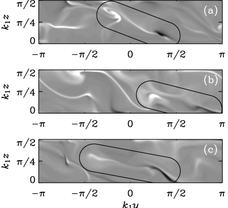
Figure 3.: Magnetograms of the radial field at the outer surface on the northern hemisphere at different times. Light shades correspond to field vectors pointing out of the domain, and dark shades correspond to vectors pointing into the domain. The elongated rings highlight the positions of bipolar regions. Note the clockwise tilt relative to the $y$ (or toroidal) direction of systematically aligned bipolar regions. [Adapted from B05.]

We have already mentioned that large scale dynamo action is possible for helical turbulence. The qualitative picture is well understood in the framework of mean field dynamo theory, and even its nonlinear saturation behavior is well reproduced in the absence of boundaries (Field & Blackman 2002). Thus, in sufficiently simple situations, such as these, mean field theory does actually begin to have predictive power. Even in the presence of shear, the theory with dynamical quenching formalism predicts a nonlinear behavior that is compatible with simulations (Blackman & Brandenburg 2002, Subramanian 2002).

Shear leads to two important effects. The first one was long known: the amplification of a toroidal field from a poloidal one. The second is far less obvious and has only recently been discussed: the transport of magnetic and current helicity along lines of constant angular velocity (Vishniac & Cho 2001, Subramanian & Brandenburg 2004). Qualitatively, any large scale dynamo, even if the turbulence is not driven helically, does imply the production of small scale magnetic and current helicities, which tends to ‘suffocate’ the large scale dynamo process (Brandenburg et al. 2002). In order to prevent this from happening, it is important to expel small scale magnetic and current helicity, e.g. via transport along linear of constant angular velocity, which is why this shear is so important. That this actually makes a tremendous difference becomes clear from Fig. 2, where we show the growth of magnetic energy contained in the total field, $\langle{\bm{B}}^{2}\rangle$, and the mean field, $\langle\overline{\bm{B}}^{2}\rangle$. Here, overbars denote averages over a meridional plane and angular brackets denote volume averages. All models have the same amount of shear, some models have helical forcing of the turbulence while others have non-helical forcing; this does not make a big difference as far as the generation of magnetic energy is concerned (cf. solid and dashed lines in the inset of Fig. 2). Furthermore, there is one model that has closed boundaries – preventing the generated magnetic and current helicities to escape (dashed line in main part of plot). The effect is dramatic! Both large scale and small scale fields saturate at a level that is well below the equipartition value – in stark contrast to the case with open boundaries.

Finally we discuss the topology of the generated magnetic field, as viewed at the outer surface of the domain; see Fig. 3. The magnetic field appears to be tube-like at the outer surface, even though meridional cross-sections of the field show a rather smooth field distribution (see Fig. 4 of B05). This suggests that the localized appearance the field is primarily produced close to the boundary. Furthermore, the field appears in the form of bipolar regions with a systematic tilt angle. Here the tilt is produced by latitudinal shear, which causes all points closer to the equator to drift faster than those further away (see B05 for details).

3. Conclusion

The main point of this discussion is to stress that the solar dynamo may well work in the bulk of the convection zone. The near surface shear may not only be responsible for east-west alignment and toroidal field production, but it may also play a role in disposing of small scale magnetic and current helicities from the dynamo, e.g. via coronal mass ejections (Blackman & Brandenburg 2003).

References

- (1) Benevolenskaya, E. E., Hoeksema, J. T., Kosovichev, A. G., et al. 1999, ApJ, 517, L163
- (2) Blackman, E. G., & Brandenburg, A. 2002, ApJ, 579, 359
- (3) Blackman, E. G., & Brandenburg, A. 2003, ApJ, 584, L99
- (4) Boldyrev, S., & Cattaneo, F. 2004, PRL, 92, 144501
- (5) Brandenburg, A. 2001, ApJ, 550, 824
- (6) Brandenburg, A. 2005, ApJ, 625, 539 (B05)
- (7) Brandenburg, A., Dobler, W., & Subramanian, K. 2002, AN, 323, 99
- (8) Brun, A. S., Miesch, M. S. & Toomre, J. 2004, ApJ, 614, 1073
- (9) Choudhuri, A. R. 1990, ApJ, 355, 733
- (10) Field, G. B., & Blackman, E. G. 2002, ApJ, 572, 685
- (11) Galloway, D., & Weiss, N. O. 1981, Geophys. Astrophys. Fluid Dyn., 243, 945
- (12) Golub, L., Rosner, R., Vaiana, G. S., & Weiss, N. O. 1981, ApJ, 243, 309
- (13) Haugen, N. E. L., Brandenburg, A., & Dobler, W. 2004, PRE, 70, 016308
- (14) Kitchatinov, L. L., & Mazur, M. V. 2000, Sol. Phys., 191, 325
- (15) Kleeorin, N. I., Mond, M., & Rogachevskii, I. 1996, A&A, 307, 293
- (16) Krivodubskii, V. N. 1984, Sov. Astron., 28, 205
- (17) Markiel, J. A., & Thomas, J. H. 1999, ApJ, 523, 827
- (18) Moss, D., Tuominen, I., & Brandenburg, A. 1990, A&A, 240, 142
- (19) Nordlund, Å., Brandenburg, A., Jennings, et al. 1992, ApJ, 392, 647
- (20) Parker, E. N. 1987, Sol. Phys., 110, 11
- (21) Rüdiger, G. & Brandenburg, A. 1995, A&A, 296, 557
- (22) Schekochihin, A. A., Haugen, N. E. L., Brandenburg, A., et al. 2005, ApJ, 625, L115
- (23) Spiegel, E. A., & Weiss, N. O. 1980, Nat, 287, 616
- (24) Spruit, H. C., & Zweibel, E. G. 1979, Sol. Phys., 62, 15
- (25) Stix, M. 1976, A&A, 47, 243
- (26) Subramanian, K. 2002, Bull. Astr. Soc. India, 30, 715
- (27) Subramanian, K., & Brandenburg, A. 2004, PRL, 93, 205001
- (28) Tobias, S. M., Brummell, N. H., Clune, T. L., & Toomre, J. 1998, ApJ, 502, L177
- (29) Vishniac, E. T., & Cho, J. 2001, ApJ, 550, 752
- (30) Yoshimura, H. 1976, Sol. Phys., 50, 3
- (31) Zwaan, C. 1978, Sol. Phys., 60, 213