On the Relation Between Hot Jupiters and the Roche Limit

Abstract

Many of the known extrasolar planets are “hot Jupiters,” giant planets with orbital periods of just a few days. We use the observed distribution of hot Jupiters to constrain the location of its inner edge in the mass–period diagram. If we assume a slope corresponding to the classical Roche limit, then we find that the edge corresponds to a separation close to twice the Roche limit, as expected if the planets started on highly eccentric orbits that were later circularized. In contrast, any migration scenario would predict an inner edge right at the Roche limit, which applies to planets approaching on nearly circular orbits. However, the current sample of hot Jupiters is not sufficient to provide a precise constraint simultaneously on both the location and slope of the inner edge.

1 Introduction

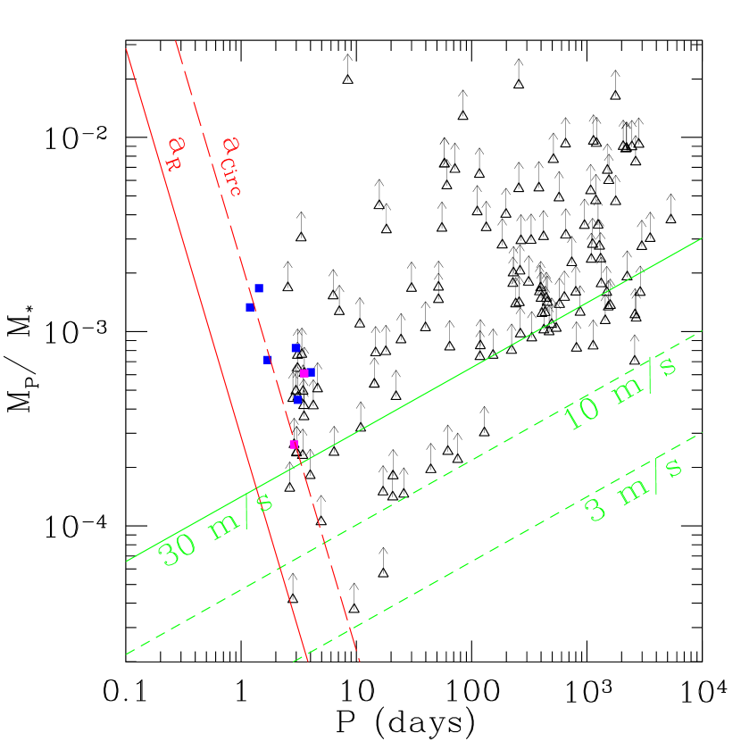
Figure 1: Minimum mass ratio vs orbital period for the current observed sample. Planets discovered by radial velocity surveys are shown as triangles with arrows indicating $1-\sigma$ uncertainties in mass due to unknown inclination. The magenta squares were discovered by radial velocity observations and have inclinations and radii measured via transits. The blue squares show planets discovered by transit searches. The green lines show the minimum mass corresponding to various velocity semi-amplitudes and roughly indicate where radial velocity surveys are nearly complete ($\geq 30\,$m/s), have significant sensitivity ($\geq 10\,$m/s), and are only beginning to detect planets ($\geq 3\,$m/s). The two red lines show the location of the Roche limit ($a_{R}$) and the ideal circularization radius ($a_{\rm circ}$) for a planet with a radius $R_{P}=1.2\,R_{J}$. The red lines do not apply to the lowest mass planets that likely have a radius significantly less than $1.2\,R_{J}$ given their different internal structure.

Early discoveries of hot Jupiters hinted at a pile-up near a 3-day period, but recent transit surveys and more sensitive radial velocity observations have discovered planets with even shorter periods. The data now suggest that the inner limit for hot Jupiters is not defined by an orbital period, but rather by a tidal limit, which depends on both the separation and the planet-star mass ratio (Fig. 1). This would arise naturally if the inner edge were related to the Roche limit, the critical distance within which a planet would start losing mass (Faber et al. 2005). The Roche limit separation, $a_{R}$, is given by $R_{P}=0.462\,a_{R}\,\mu^{1/3}$, where $R_{P}$ is the radius of the planet, and $\mu=m/M_{*}$ is the planet-star mass ratio.

The many formation scenarios proposed for hot Jupiters can be divided into two broad categories. The first involves slow migration on quasi-circular orbits, perhaps due to interaction with a gaseous disk or planetesimal scattering (Murray et al. 1998; Trilling et al.  1998). This would result in an inner edge precisely at the Roche limit. The second category invokes tidal circularization of highly eccentric orbits with very small pericenter distances, following planet-planet scattering (Rasio & Ford 1996; Weidenschilling & Marzari 1996; Ford et al. 2001; Papaloizou & Terquem 2001; Marzari & Weidenschilling 2002), secular perturbations from a wide binary companion (Holman et al. 1997; Wu & Murray 2003), or tidal capture of free-floating planets (Gaudi 2003). These would result in a limiting separation of twice the Roche limit, assuming that circularization can take place without significant mass loss from the planet (Faber et al. 2005; Gu et al. 2003; Rasio et al. 1996).

2 Statistical Analysis

To constrain rigorously the distribution of hot Jupiters, we adopt a Bayesian framework, where the model parameters are treated as random variables to be constrained by the actual observations. To perform a Bayesian analysis it is necessary to specify both the likelihood (the probability of making a certain observation given a particular set of model parameters) and the prior (the a priori probability distribution for the model parameters). Let us denote the model parameters by $\theta$ and the data by $d$, so that their joint probability distribution function (PDF) is given by $p(d,\theta)=p(\theta)p(d|\theta)=p(d)p(\theta|d).$ Note how the joint PDF is expanded in two ways, both expressed as the product of a marginalized PDF and a conditional PDF. The prior is given by $p(\theta)$ and the likelihood by $p(d|\theta)$, while $p(d)$ is the a priori probability for observing the values actually measured and $p(\theta|d)$ is the PDF of primary interest: the a posteriori PDF for the model parameters conditioned on the actual observations. The probability of the observations $p(d)$ can be obtained by marginalizing over the joint PDF and again expanding the joint density as the product of the prior and the likelihood. This leads to Bayes’ theorem, the primary tool for Bayesian inference,

$$p(\theta|d)=\frac{p(d|\theta)p(\theta)}{p(d)}=\frac{p(d|\theta)p(\theta)}{\int\,d\theta p(d|\theta)p(\theta)}$$ (1)

Often the model parameters contain a quantity of particular interest (the location of the inner cutoff for hot Jupiters in our analysis) plus other “nuisance parameters,” which are necessary to describe the observations (e.g., the fraction of stars with hot Jupiters in our analysis). Since Bayes’ theorem provides a real PDF for the model parameters, we can simply marginalize over the nuisance parameters to calculate a marginalized posterior PDF, which will be our basis for making inferences about the location of the inner cutoff for hot Jupiters.

2.0.1 1-d Model

We start by presenting a simple 1-d model for the distribution of hot Jupiters. The primary question we wish to address is the location of the inner edge of the distribution relative to the Roche limit. Therefore, we define $x\equiv a/a_{R}$, where $a$ is the semimajor axis of the planet and $a_{R}$ is the Roche limit. We assume that the actual distribution of $x$ for hot Jupiters is given by a truncated power law,

$$p(x|\gamma,x_{l},x_{u})dx=x^{\gamma}\left(\frac{dx}{x}\right),\quad x_{l}<x<x_{u},$$ (2)

and zero elsewhere. Here $\gamma$ is the power-law index and $x_{l}$ and $x_{u}$ are the lower and upper limits for $x$. The lower limit, $x_{l}$, is the model parameter of primary interest, while $\gamma$ and $x_{u}$ are nuisance parameters. Therefore, our results are contained in the marginalized posterior PDF for $x_{l}$.

For simplicity we restrict our analysis to the subset of known extrasolar planets discovered by complete radial-velocity surveys, extremely unlikely to contain any false positives. To obtain such a sample, we impose two constraints: $P\leq P_{\max}$, where $P_{\max}$ is a maximum orbital period, and $K\geq K_{\min}$, where $K_{\min}$ is a minimum velocity semi-amplitude. We use $K_{\min}=30$m/s, following Cumming (2004). We typically set $P_{\max}=30\,$d, even though radial-velocity surveys are likely to be complete for even longer periods (provided $K\geq K_{\min}$). This minimizes the chance of introducing biases due to survey incompleteness or possible structure in the observed distribution at larger periods. By considering only planets with orbital parameters such that radial- velocity surveys are very nearly complete, our analysis does not depend on the velocities of stars for which no planet has been detected. Note that our criteria for including a planet may introduce a bias depending on the actual mass-period distribution. We will address this with a 2-d model below. Note that, in this paper, we exclude any planet discovered via techniques other than radial velocities (e.g., transits), even if subsequent radial-velocity observations were obtained to confirm the planet.

Initially, we make several simplifying assumptions to allow for a simple analytic treatment. We assume uniform priors for each of the model parameters, $p(\gamma)\sim U(\gamma_{\min},\gamma_{\max})$ and $p(x_{l},x_{u})\sim\mathrm{const}$, provided $x_{ll}<x_{l}<x_{u}<x_{uu}$ and zero otherwise. The lower and upper limits are chosen to be sufficiently far removed from regions of high likelihood that these choices do not affect our results. We assume that the orbital period ($P$), velocity semi-amplitude ($K$), semi-major axis ($a$), stellar mass ($M_{*}$), and planet mass ($m\sin i$) are known exactly based on the observations.

We begin by assuming that $\sin i=1$ (orbital plane seen nearly edge- on) for all systems and that all planets have the same radius, $R_{P}$. With these assumptions, the posterior probability distribution is

$$p(x_{l},x_{u},\gamma|x_{1},...x_{n})\sim\gamma^{n}(x_{u}^{\gamma}-x_{l}^{\gamma})^{-n}\prod_{j=1}^{n}x_{j}^{\gamma-1},$$ (3)

provided that $x_{ll}<x_{l}\leq x_{(1)}\leq x_{(n)}\leq x_{u}<x_{uu}$ and $\gamma_{\min}<\gamma<\gamma_{\max}$. Here $n$ is the number of planets included in the analysis, $x_{(1)}$ is the smallest value of $x$ among the planets used in the analysis, and $x_{(n)}$ is the largest value. The normalization can be obtained by integrating over all allowed values of $x_{l}$, $x_{u}$, and $\gamma$. We show the marginal posterior distributions after integrating over the nuisance parameters, $x_{u}$ and $\gamma$, in Fig. 2 (dotted line), assuming $R_{P}=1.2\,R_{J}$. The distribution has a sharp cutoff at $x_{(1)}$ and a tail to lower values reflecting the chance that $x_{l}<x_{(1)}$ due to the finite sample size.

Next, we adopt an isotropic distribution of inclinations ($\cos i\sim~{}U[-1,1]$), but we use the measured value for radial-velocity planets where the orbital inclination has been determined via transits. We show the marginal posterior distribution for $x_{l}$ in Fig. 2 (solid line). The sharp cutoff at $x_{(1)}$ is replaced with a more gradual tail, reflecting the chance that $\sin i<1$ for planets with the smallest values of $x$.

Now consider the consequences of allowing for a distribution of planetary radii. For transiting planets we use a normal distribution based on the published radius value and uncertainty. For non-transiting planets, we assume a normal distribution with standard deviation $\sigma_{R_{P}}$. We show the resulting marginalized posterior PDFs in Fig. 2. Allowing for a significant dispersion broadens the posterior distribution for $x_{l}$ and results in a slight shift to smaller values. We have also explored the effects of varying the model parameter $P_{\max}$ from $8\,$d to $60\,$d. We find that this does not produce any discernible difference in the posterior PDF for $x_{l}$.

Our results are sensitive to the choice of mean radius for the non-transiting planets. In Fig. 3 (upper) we show the posterior PDFs for various mean radii, assuming $\sigma_{R_{P}}=0.1\,R_{J}$. Since few planets have a known inclination, there is a nearly perfect degeneracy between $R_{P}$ and $x_{l}$. Even when we include transiting planets, this degeneracy remains near perfect, i.e., $p(x_{l}|R_{p},x_{1},...,x_{n})\simeq p(x_{l}\cdot\frac{R^{\prime}_{P}}{R_{P}}|R^{\prime}_{P},x_{1},...,x_{n})$. However, it remains extremely unlikely that $x_{l}\simeq 1$ for any reasonable planetary radius.

2.0.2 2-d Model

We can improve our analysis by more properly considering the joint PDF in orbital period and planet-star mass ratio, which we write as

$$p(P,\mu|\alpha,\beta,P_{\min},P_{\max},\mu_{\min},\mu_{\max},c)\sim cP^{\alpha}\mu^{\beta}\frac{dP}{P}\frac{d\mu}{\mu},$$ (4)

provided $\mu_{\min}<\mu<\mu_{\max}$, $P<P_{\max}$, and $a(P,M_{*})\geq x_{l}\cdot a_{R}(R_{P},\mu)$. Here $\alpha$ and $\beta$ are new power-law indices. Again our results are not sensitive to the nuisance parameters, $\mu_{\min}$, $\mu_{\max}$, and $P_{\max}$. For definiteness, we fix their values at $P_{\max}=30\,$d, $\mu_{\min}=3.3\times 10^{-5}$, and $\mu_{\max}=0.01$. We take priors uniform in $\tan^{-1}(\alpha)$ and $\tan^{-1}(\beta)$, as the density $U[-\pi/2,\pi/2]$ corresponds to uniform prior density for the slope of the power-law distribution on a log-log plot. We take a prior uniform in $\log c$, as is standard for scale parameters. Our calculation of the likelihood is similar to that of Tabachnik & Tremaine (2002), except we replaced their inner boundary of $P\geq P_{\min}$ with our boundary $a(P,M_{*})\geq x_{l}a_{R}(R_{P},\mu)$. The necessary integrals can be performed analytically provided we approximate $1+\mu\simeq 1$. For convenience we used Maple to obtain an analytic expression for the integral of the likelihood over $P$ and $\mu$. The remaining integrals over $\alpha$, $\beta$, and $c$ were performed numerically over a grid with $\sim 10^{10}$ points.

By considering the joint mass-period PDF, we are able to account for the bias previously introduced by imposing $K\geq K_{\max}$. Since we are considering only planets with orbital parameters such that radial-velocity surveys are very nearly complete, our results depend only on the number of surveyed stars for which no planet has been discovered, and not the observed velocities of these stars. For the total number of stars in radial-velocity surveys that are complete for $K\geq K_{\min}$ and $P\leq P_{\max}$ we estimate $N_{*}=2000$. We show the resulting marginalized posterior PDF for $x_{l}$ in Fig. 3 (lower).

2.0.3 The Shape of the Inner Cutoff

The above results clearly demonstrate that the present observations strongly favor an inner cutoff at the ideal circularization distance rather than at the Roche limit, assuming that the inner edge follows the slope of the Roche limit. We have also performed calculations treating this slope as an unknown model parameter. Unfortunately, the present observations are not sufficient to constrain this parameter empirically, and the resulting marginalized posterior PDF for $x_{l}$ still allows, but no longer exclusively favors, $x_{l}\simeq 2$.

We could gain additional leverage by including planets in short-period orbits down to lower $K_{\min}$. Unfortunately, the incompleteness of the radial-velocity surveys is likely to be significant for $K_{\min}<20\,$m/s. Since the number, quality, and spacing of observations varies widely among the stars in these surveys, it would be necessary to calculate the probability for detecting planets as a function of orbital period and velocity semi-amplitude for each star. Additionally, the planet mass-radius relation, which is extremely flat for planets near $1\,M_{J}$, becomes important for much lower-mass planets. Therefore, we have not attempted to extend our analysis to planets for which radial-velocity surveys are not yet complete. We expect that the recent improvements in measurement precision will eventually extend their completeness to smaller $K_{\min}$.

We have begun a preliminary investigation of the constraints obtained by adding information from the OGLE transit survey (Udalski 2002). Due to both signal-to-noise and aliasing issues, the OGLE survey does not provide a complete sample of short-period planets for a significant fraction of parameter space. Therefore, it is necessary to calculate the probability of detecting planets with various orbital periods and radii. We estimate these probabilities by taking the actual observation times and uncertainties for the 62 transit candidates from the 2002 OGLE observations of the Carina field and applying the detection criteria from Pont et al. (2005). While the transiting planets are consistent with our above findings, they do not provide sufficient additional information to constrain the slope of the inner edge. We look forward to both radial-velocity and transit surveys detecting additional lower-mass objects in short-period orbits, so that we may eventually constrain the slope of the cutoff empirically.

3 Discussion

The current distribution of hot Jupiters shows a cutoff that is a function of orbital period and planet mass. Under the assumption that the slope of this cutoff follows the Roche limit, our Bayesian analysis solidly rejects the hypothesis that the cutoff occurs inside or at the present Roche limit. This is in constrast to what would be expected if these planets had slowly migrated inwards on quasi-circular orbits and with radii close to the presently measured values around $1.2\,R_{J}$. If confirmed by future analyses of a more extensive data set, this result would be highly significant, as it would eliminate a broad class of popular migration scenarios for the formation of hot Jupiters.

Instead, our analysis shows that this cutoff occurs at a distance nearly twice that of the Roche limit, as expected if the planets had been circularized from a highly eccentric orbit. These findings suggest that hot Jupiters may have formed via planet-planet scattering (Rasio & Ford 1996), tidal capture of free floating planets (Gaudi 2003), or secular perturbations from a highly inclined binary companion (Holman et al. 1997). Regardless of the exact mechanism, our model would require that the hot Jupiters all started on highly eccentric orbits and survived the strong tidal dissipation needed to circularize their orbits. A few caveats are worth mentioning. Our study addresses the statistical properties of the population of hot-Jupiters and does not attempt to advance the state of knowledge of any specific planet. In particular, we adopt average properties of an assumed distribution that is analogous to—and derived from—the presently known distribution of hot Jupiters, but we do not consider or solve for the specific properties of any individual extrasolar planet. Moreover, strongly non-random or non-gaussian effects would be poorly modeled with the technique developed here.

An alternative explanation is that the planets migrated inwards at an early time and arrived at their Roche limit on a quasi-circular orbit when their radii were still $\geq 2\,R_{J}$ (Burrows et al. 2000). The dissipation process causing the migration must then have stopped immediately afterwards to avoid further decay of the orbit as the planets continued to cool and contract. We find this scenario unattractive, especially since there is no natural explanation for the factor of 2 in this case.

Yet another alternative is that short-period giant planets are destroyed by some process before they reach the Roche limit. HST observations of HD 209458 indicate absorption by matter presently beyond the Roche lobe of the planet and have been interpreted as evidence for a wind leaving the planet and powered by stellar irradiation (Vidal-Madjar et al. 2003, 2004). Further theoretical work will help determine under what conditions these processes can cause significant mass loss (e.g., Hubbard et al. 2005) and whether complete destruction could occur rather suddenly when the orbital radius decreases below $\sim 2a_{R}$.

Future planet discoveries will either tighten the constraints on the model parameters or provide evidence for the existence of planets definitely closer than twice the Roche limit. Additionally, future discoveries of transiting hot-Jupiters around young stars could help discriminate between the above alternatives. Moreover, new detections of lower-mass planets with very short periods could help better constrain the shape of the inner cutoff as a function of mass. In the future, an improved statistical analysis could also include such low- mass planets, where surveys are not yet complete.

Figure 2: Marginalized posterior probability distribution for $x_{l}$, the lower cutoff for the ratio of a planet’s semimajor axis to the Roche limit. Here we show multiple posterior distributions for various simplified models. The dotted curve assumes $R_{P}=1.2\,R_{J}$ and $\sin i=1$ for all planets, while the remaining lines assume the observed inclinations and radii for transiting planets and an isotropic distribution of inclinations and mean radius $R_{P}=1.2\,R_{J}$ for the remaining planets. The widths of the distributions in radii are $0.0R_{J}$ (dotted and solid curves), $0.05R_{J}$ (long dashes), $0.1R_{J}$ dots-dashes), $0.2R_{J}$ (short dashes).

Figure 3: Posterior distributions from our 1-d model (top) and full 2-d model (bottom) for various mean radii: $\left<R_{P}\right>=1.0R_{J}$ (long dashes), $1.1R_{J}$ (dotted), $1.2R_{J}$ (solid), $1.3R_{J}$ (dotted dashed), and $1.4R_{J}$ (short dashes), all assuming $\sigma_{R_{P}}=0.1R_{J}$.

References

- (1) Burrows, A., et al. 2000, ApJ, 534, 97
- (2)
- (3) Cumming, A. 2004, MNRAS, 354, 1165
- (4)
- (5) Faber, J.A., Rasio, F.A. & Willems, B. 2005, Icarus, 175, 248
- (6)
- (7) Ford, E.B., Havlickova, M., & Rasio, F.A. 2001, Icarus, 150, 303
- (8)
- (9) Gaudi, S. 2003, astro-ph/0307280.
- (10)
- (11) Gu, P.-G., Lin, D.N.C. & Bodenheimer P.H. 2003, ApJ, 558, 509
- (12)
- (13) Holman, M., Touma, T. & Tremaine, S. 1997, Nature, 386, 254
- (14)
- (15) Hubbard, W.B., Hattori, M.F., Burrows, A., Hubeny, I., & Sudarsky, D. 2005, astro-ph/0508591
- (16)
- (17) Marzari, F. & Weidenschilling, S.J. 2002, Icarus 156, 670
- (18)
- (19) Murray, N., Hansen, B., Holman, M., & Tremaine, S. 1998, Science, 279, 69
- (20)
- (21) Papaloizou, J.C.B. & Terquem, C. 2001, MNRAS, 325, 221
- (22)
- (23) Pont et al. 2005, A&A 438, 1123
- (24)
- (25) Rasio, F.A. & Ford, E.B. 1996, Science, 274, 954
- (26)
- (27) Rasio, F.A., Tout, C.A., Lubow, S.H., & Livio, M. 1996, ApJ, 470, 1187
- (28)
- (29) Tabachnik, S. & Tremaine, S. 2002, MNRAS 335, 151
- (30)
- (31) Trilling et al. 1998, ApJ, 500, 428
- (32)
- (33) Udalski et al. 2002, Acta Astron., 52, 1
- (34)
- (35) Vidal-Madjar, A., Lecavelier des Etangs, A., Desert, J.- M., Ballester, G.E., Ferlet, R., Hebrand, G., Mayor, M. 2003, Nature, 422, 143
- (36)
- (37) Vidal-Madjar, A. et al. 2004, ApJL 604, 69
- (38)
- (39) Weidenschilling, S.J., & Marzari, F. 1996, Nature, 384, 619
- (40)
- (41) Wu, Y., & Murray, N. 2003, ApJ, 589, 605
- (42)