The Importance of Off-Jet Relativistic Kinematics in Gamma-Ray Burst Jet Models

Abstract

Gamma-Ray Bursts (GRBs) are widely thought to originate from collimated jets of material moving at relativistic velocities. Emission from such a jet should be visible even when viewed from outside the angle of collimation. I summarize recent work on the special relativistic transformation of the burst quantities $E_{\rm iso}$ and $E_{\rm peak}$ as a function of viewing angle, where $E_{\rm iso}$ is the isotropic-equivalent energy of the burst and $E_{\rm peak}$ is the peak of the burst spectrum in the power $\nu F_{\nu}$. The formulae resulting from this work serve as input for a Monte Carlo population synthesis method, with which I investigate the importance of off-jet relativistic kinematics as an explanation for a class of GRBs termed “X-ray Flashes” (XRFs). I do this in the context of several top-hat shaped variable opening-angle jet models. I find that such models predict a large population of off-jet bursts that are observable and that lie away from the $E_{\rm peak}\propto E_{\rm iso}^{1/2}$ relation. The predicted burst populations are not seen in current datasets. I investigate the effect of the bulk $\gamma$ value upon the properties of this population of off-jet bursts, as well as the effect of including an $\Omega_{0}$-$E_{\gamma}$ correlation to jointly fit the $E_{\rm peak}\propto E_{\rm iso}^{1/2}$ and $E_{\rm peak}\propto E_{\gamma}^{\beta}$ relations, where $\Omega_{0}$ is the opening solid angle of the GRB jet. I find that the XRFs seen by HETE-2 and BeppoSAX cannot be easily explained as classical GRBs viewed off-jet. I also find that an inverse correlation between $\gamma$ and $\Omega_{0}$ has the effect of greatly reducing the visibility of off-jet events. Therefore, unless $\gamma>300$ for all bursts or unless there is a strong inverse correlation between $\gamma$ and $\Omega_{0}$, top-hat variable opening-angle jet models produce a significant population of bursts away from the $E_{\rm peak}\propto E_{\rm iso}^{1/2}$ and $E_{\rm peak}\propto E_{\gamma}^{\beta}$ relations, in contradiction of current observations.

1. Introduction

The importance of collimated jets in GRBs was highlighted by the extremely large isotropic-equivalent energies ($E_{\rm iso}$) of very luminous events like GRB 971214 (Kulkarni et al., 1998) and GRB 990123 (Kulkarni et al., 1999) and by the observation of breaks in afterglow light-curves (Rhoads, 1997; Sari, Piran & Halpern, 1999; Harrison et al., 1999). Frail et al. (2001) and Bloom et al. (2003) corrected the isotropic-equivalent energies by the beaming fraction obtained from the jet break time in afterglow light-curves and found that the values of the energy released in $\gamma$-rays ($E_{\gamma}$) were tightly clustered around $10^{51}$ ergs. Recently Ghirlanda et al. (2004) have shown that a tight correlation exists between $E_{\gamma}$ and the peak of the $\nu F_{\nu}$ spectrum in the rest-frame, $E_{\rm peak}$. Recent results by Sakamoto et al. (2005a) obtained from HETE-2 (Ricker et al., 2001) observations have shown that XRFs (Heise et al., 2001; Kippen et al., 2001), X-ray-rich GRBs and GRBs lie along a continuum of properties and that XRFs with known redshift extend the $E_{\rm peak}\propto E_{\rm iso}^{1/2}$ relation predicted by Lloyd-Ronning et al. (2000) and found by Amati et al. (2002) to over five orders of magnitude in $E_{\rm iso}$ (Lamb et al., 2005).

Relativistic kinematics implies that even a “top-hat”-shaped jet will be visible when viewed outside its angle of collimation; i.e., off-jet (Ioka & Nakamura, 2001). Yamazaki, Ioka & Nakamura (2002, 2003) used this fact to construct a model where XRFs are simply classical GRBs viewed at an angle $\theta_{\rm v}>\theta_{0}$, where $\theta_{0}$ is the half-opening angle of the jet and $\theta_{\rm v}$ is the angle between the axis of the jet and the line-of-sight. The authors showed that such a model could reproduce many of the observed characteristics of XRFs. Yamazaki, Ioka & Nakamura (2004a) showed that in such a model, the distribution of both on- and off-jet observed bursts was roughly consistent with the $E_{\rm peak}\propto E_{\rm iso}^{1/2}$ relation.

In this paper, I use the population synthesis method developed by Lamb, Donaghy, & Graziani (2005) and incorporate the relativistic emission profiles calculated by Graziani et al. (2005), to predict the global properties of bursts localized by HETE-2 and BeppoSAX. I consider the possibility that the XRFs observed by HETE-2 and BeppoSAX are primarily regular GRBs observed off-jet (Yamazaki, Ioka & Nakamura, 2004a) and show that it is difficult to account for the observed properties of XRFs in this model. However, since the effect of special relativity on off-jet emission must exist, I seek to understand its relative importance in the context of current models of GRB jets. I revisit the top-hat variable opening-angle (THVOA) jet model put forward in Lamb, Donaghy, & Graziani (2005), now including the effects of relativistic kinematics on off-jet emission. I present results for several models which explore various regions of the parameter space in $\gamma$, $E_{\gamma}$ and $\theta_{0}$.

For this paper, I only consider the effect of relativistic kinematics on off-jet emission from uniform or “top-hat” jets; we will consider the effects on Fisher-shaped (Donaghy, Lamb, & Graziani, 2005a) and Gaussian-shaped (Zhang et al., 2004) jets in a future publication (Donaghy, Lamb, & Graziani, 2005b). I describe my population synthesis method in §2 and present the results for various models in §3. I discuss the results in §4 and draw some conclusions in §5. Preliminary results were reported in Donaghy (2005a).

2. Method

2.1. Off-Jet Relativistic Kinematic Formulae

Relativistic kinematics causes frequencies in the rest frame of the jet to appear Doppler shifted by a factor $\delta=\gamma(1-\beta\cos\theta)$, where $\beta$ is the bulk velocity of the jet and $\theta$ is the angle between the direction of motion and the source frame observer. The simulations I describe chiefly deal with the kinematic transformation of two important burst quantities, $E_{\rm iso}$ and $E_{\rm peak}$, as a function of viewing angle, $\theta_{\rm v}$. In the simplest “toy” model, these quantities transform as $E_{\rm peak}\propto\delta^{-1}$ and $E_{\rm iso}\propto\delta^{-3}$, from which arises the relation $E_{\rm peak}\propto E_{\rm iso}^{1/3}$ (Yamazaki, Ioka & Nakamura, 2002). In the more complete model of Graziani et al. (2005), this relation is satisfied only in the limit $\theta_{\rm v}\gg\theta_{0}$.

The complete relativistic kinematic expressions involve convolution of the Doppler function and the intrinsic profile of the jet. For an arbitrary smooth profile, an efficient algorithm exists to calculate the profiles; for the case I am interested in, the uniform or “top-hat” profile, a closed analytic expression can be given. The formulae are derived in Graziani et al. (2005), and I summarize them below. The current model differs slightly from that used by Yamazaki, Ioka & Nakamura (2004a) in that we consider steady-state emission, rather than the evolution of burst properties due to time-of-flight effects. The model therefore applies to burst-averaged data products like $E_{\rm iso}$ and $E_{\rm peak}$.

The observed isotropic-equivalent energy, $E_{\rm iso}$, of the jet as a function of $\theta_{\rm v}$ is given by,

$$E_{\rm iso}=\frac{E^{\rm true}_{\gamma}}{2\beta\gamma^{4}(1-\cos\theta_{0})}\left[f(\beta-\cos\theta_{\rm v})-f(\beta\cos\theta_{0}-\cos\theta_{\rm v})\right],$$ (1)

where

$$f(z)=\frac{\gamma^{2}(2\gamma^{2}-1)z^{3}+(3\gamma^{2}\sin^{2}\theta_{\rm v})z+2\cos\theta_{\rm v}\sin^{2}\theta_{\rm v}}{(z^{2}+\gamma^{-2}\sin^{2}\theta_{\rm v})^{3/2}},$$ (2)

and $E^{\rm true}_{\gamma}$ is the total energy emitted by the jet in gamma rays and serves as the energy scale for the emission profile.

The transformation of $E_{\rm peak}$ as a function of $\theta_{\rm v}$ is slightly more complicated. The detailed physics underlying the prompt emission of gamma-ray bursts is not yet well understood. In particular, an explanation of the prompt emission spectrum (apparently universally parametrized by the Band function (Band et al., 1993)) is currently lacking. The observed spectrum (including the value of $E_{\rm peak}$) is almost certainly due to superpositions of emission from different regions on the jet, convolved with relativistic kinematic effects. A detailed explanation of how this forms a Band spectrum is beyond the scope of this paper. Instead we calculate the average Doppler shift across the jet as a proxy for $E_{\rm peak}$. The average shift, $\langle D\rangle$, is given by,

$$\langle D\rangle=\gamma^{-1}\frac{f(\beta-\cos\theta_{\rm v})-f(\beta\cos\theta_{0}-\cos\theta_{\rm v})}{g(\beta-\cos\theta_{\rm v})-g(\beta\cos\theta_{0}-\cos\theta_{\rm v})},$$ (3)

where

$$g(z)=\frac{2\gamma^{2}z+2\cos\theta_{\rm v}}{(z^{2}+\gamma^{-2}\sin^{2}\theta_{\rm v})^{1/2}}.$$ (4)

$E_{\rm peak}$ is related to $\langle D\rangle$ via,

$$E_{\rm peak}=\langle D\rangle\times E_{\rm peak}^{\rm(rest)},$$ (5)

where $E_{\rm peak}^{\rm(rest)}$ is the (unknown) peak energy of the burst spectrum in the rest frame. We remove this unknown normalization by requiring all bursts to obey the $E_{\rm peak}\propto E_{\rm iso}^{1/2}$ relation at the center of the jet, thereby fixing this normalization to that of $E_{\rm iso}$. Thus,

$$E_{\rm peak}=\frac{\langle D(\theta_{\rm v})\rangle}{\langle D(0)\rangle}\cdot E_{\rm peak}^{(\rm on)}=\frac{\langle D(\theta_{\rm v})\rangle}{\langle D(0)\rangle}\cdot C_{A}\cdot\left(E_{\rm iso}^{(\rm on)}/E_{A}\right)^{0.5},$$ (6)

where $E_{\rm iso}^{(\rm on)}$ is simply Equation 1 evaluated at $\theta_{\rm v}=0$. Figure 1 shows $E_{\rm iso}$ and $\langle D\rangle$ plotted as functions of $\theta_{\rm v}$ for various values of $\theta_{0}$ and $\gamma$, and Figure 2 shows the corresponding trajectories in the [$E_{\rm iso}$,$\langle D\rangle$]-plane as $\theta_{\rm v}$ increases away from the jet axis.

Figure 1.— Emission profiles (top row) and average Doppler shift (bottom row) as a function of viewing angle, for a range of $\gamma$ and $\theta_{0}=0.1$ rad (left) and $\theta_{0}=0.01$ rad (right). From Graziani et al. (2005).

Figure 2.— Trajectories in the [$E_{\rm iso}$,$\langle D\rangle$]-plane (“Amati plot”), moving from right to left as $\theta_{\rm v}$ increases, for $\theta_{0}=0.1$ rad (left) and $\theta_{0}=0.01$ rad (right). The axes are scaled so that a $45^{\circ}$ line corresponds to a slope of $1/2$. From Graziani et al. (2005).

2.2. Monte Carlo Simulations

The population synthesis Monte Carlo simulations described in this paper follow the method presented in Lamb, Donaghy, & Graziani (2005). Beginning in the rest-frame of each burst I specify $\theta_{0}$, $E^{\rm true}_{\gamma}$ and $\gamma$ by drawing from various input distributions (depending on the model used). A value for $\theta_{\rm v}$ is drawn from the distribution $dN=\sin(\theta_{\rm v})\;d\theta_{\rm v}$. I then calculate $E_{\rm iso}$ and $E_{\rm peak}$ from Equations 1 and 6.

I also introduce two Gaussian smearing functions to add a stochastic element to the simulations. I draw values for the coefficient $C_{A}$ in Equation 6 from a narrow lognormal distribution to model the observed width of the $E_{\rm peak}\propto E_{\rm iso}^{1/2}$ relation. Another narrow lognormal distribution is used to generate a timescale for each burst that converts fluences to peak fluxes. For both of these Gaussians I use the same parameters as in Lamb, Donaghy, & Graziani (2005).

I then draw redshift values from a model for the star-formation rate (Rowan-Robinson, 2001), transform the burst quantities to the observer-frame and construct a Band spectrum (assuming $\alpha=-1$ and $\beta=-2.5$). Using the observer-frame Band spectrum I can calculate photon and energy fluences and peak fluxes in any desired passband. By comparing with the peak photon flux thresholds as described by Band (2003), I determine if a burst would be detected by a given instrument. In this work, I primarily employ the detector thresholds from the WXM on HETE-2, scaled to include triggers on timescales up to $5$ sec.

One change in the method from Lamb, Donaghy, & Graziani (2005) is necessarily the treatment of off-jet events. In that paper, simulation of all off-jet events was bypassed by drawing from a power-law distribution in $\Omega_{0}$ with index $\delta_{\rm sim}=\delta_{\rm true}-1$; as discussed in that work, this is equivalent to working in the $\gamma\to\infty$ limit. In that paper, we concluded that the data requested a model with approximately equal numbers of bursts per decade in all observed burst quantities, corresponding to $\delta_{\rm sim}=1$. Equivalently, in this paper I draw from a power-law distribution in $\Omega_{0}$ with index $\delta_{\rm true}=2$, and simulate the distribution of viewing angles, $\theta_{\rm v}$, to determine which off-jet events are detected.

The vast majority of jets are observed from large viewing angles and therefore are extremely faint and are not detected. In order to increase the percentage of detected bursts in a Monte Carlo sample of $50,000$ events, I do not simulate bursts that lie in regions of parameter space that produce faint bursts; i.e. bursts with values of $\theta_{\rm v}$ which are large compared to $\theta_{0}$. For each model, I plot bursts in the [$\theta_{0}$,$\theta_{\rm v}$]-plane, showing the outline of the truncated region. The models in Lamb, Donaghy, & Graziani (2005) correspond to removing all bursts above the line $\theta_{0}=\theta_{\rm v}$.

2.3. Comparison to Burst Data

To test the viability of various jet models, I compare my results against several available datasets. Considering the sample of bursts with known redshifts (localized by BeppoSAX, HETE-2 or other detectors) there are two correlations of interest between source frame quantities.

Amati et al. (2002) reported a correlation between $E_{\rm peak}$ and $E_{\rm iso}$

$$E_{\rm peak}=C_{A}\left(\frac{E_{\rm iso}}{E_{A}}\right)^{\alpha},$$ (7)

that has been confirmed and extended to over five orders of magnitude in $E_{\rm iso}$ (Sakamoto et al., 2004, 2005a; Lamb et al., 2005). I work with the best-fit value of $C_{A}=89.1\pm 8.2$ keV (fixing $\alpha=0.5$ and $E_{A}=10^{52}$ ergs) from Lamb, Donaghy, & Graziani (2005). For each realization, I draw a value for $C_{A}$ from a lognormal distribution with a width of $0.13$ decades.

Recent works (Nakar & Piran, 2004; Band & Preece, 2005) have claimed that large percentages of BATSE bursts are incompatible with the $E_{\rm peak}\propto E_{\rm iso}^{1/2}$ relation (but see Ghirlanda et al. (2005a), Bosnjak et al. (2005) and Lamb et al. (2005)). Since bursts seen away from the $E_{\rm peak}\propto E_{\rm iso}^{1/2}$ relation may be a signature of off-jet events, comparison with this relation is an important test for these models.

Using bursts with known redshift and well-measured jet-break times, Ghirlanda et al. (2004) have found a second relation

$$E_{\rm peak}=C_{G}\left(\frac{E_{\gamma}}{E_{G}}\right)^{\beta},$$ (8)

with current best-fit values of $\beta=0.69\pm 0.04$, $C_{G}=250\pm 100$ keV and $E_{G}=3.8\times 10^{50}$ ergs (Ghirlanda et al., 2005b). In §3.3 I describe the observational implications of models that satisfy both the $E_{\rm peak}\propto E_{\rm iso}^{1/2}$ and $E_{\rm peak}\propto E_{\gamma}^{\beta}$ relations.

I define the value of $E_{\gamma}$ measured using the method of Frail et al. (2001) to be $E^{\rm inf}_{\gamma}=E_{\rm iso}(1-\cos\theta_{\rm br})$, where $\theta_{\rm br}=\max(\theta_{\rm v},\theta_{0})$. The presence of off-jet emission (or any non-uniform profile) implies $E^{\rm inf}_{\gamma}\neq E^{\rm true}_{\gamma}$; in fact, $E^{\rm inf}_{\gamma}$ varies with $\theta_{\rm v}$ for a given jet, while $E^{\rm true}_{\gamma}$ is an intrinsic property of the jet.

The burst properties presented in the source frame ($E_{\rm iso}$ or $E^{\rm inf}_{\gamma}$ against $E_{\rm peak}$, or cumulative distributions of these quantities) are essentially those presented by Ghirlanda et al. (2004), augmented where appropriate with events compiled by Friedman & Bloom (2004), more recent fits to HETE-2 data from Sakamoto et al. (2005a), and a few recent Swift bursts with fits reported in GCN Circulars (Golenetskii et al., 2005a, b, c).

I also consider the larger sample of HETE-2 localized bursts with and without known redshifts (Barraud et al., 2003; Sakamoto et al., 2005a). This sample also shows a prominent hardness-intensity correlation, although it is broader than the source-frame correlation. This sample has the advantage of having many more XRFs than the sample with known redshifts. Figure 3 shows both the observer frame and source frame datasets, with the relevant correlations.

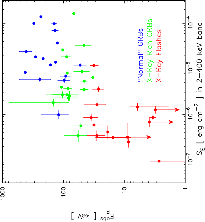
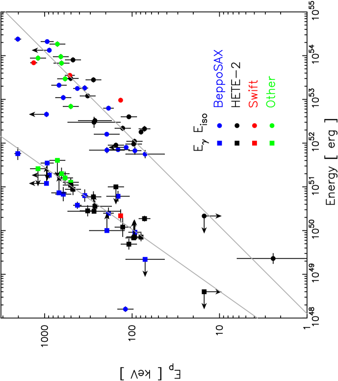
Figure 3.— Top panel shows the sample of bursts localized by the WXM on HETE-2 in the [$S_{E}$(2-400 keV),$E^{\rm obs}_{\rm peak}$]-plane, broken down into XRFs, X-ray-rich GRBs and GRBs (data taken from Sakamoto et al. (2005a) and Barraud et al. (2003)). Bottom panel shows the $E_{\rm peak}\propto E_{\rm iso}^{1/2}$ and $E_{\rm peak}\propto E_{\gamma}^{\beta}$ relations in the source frame (data taken from Ghirlanda et al. (2004), Friedman & Bloom (2004), Sakamoto et al. (2005a) and recent Swift bursts).

3. Results

Here I explore the relative importance of off-jet relativistic kinematics for six top-hat variable opening-angle jet models. In what follows, bursts that are detected by the WXM for which $\theta_{\rm v}<\theta_{0}$ are shown as blue dots (on-jet events), while detected bursts for which $\theta_{\rm v}>\theta_{0}$ are shown as green dots (off-jet events). Bursts in the simulation which are not detected are shown as red dots.

3.1. Yamazaki, Ioka & Nakamura (2004a) Model

In the first model I consider (Y04), I adopt the parameters from Yamazaki, Ioka & Nakamura (2004a). This model attempts to explain classical GRBs in terms of the variation of jet opening-angles, while XRFs are interpreted as classical GRBs viewed off-jet. The Y04 model assumes $\gamma=100$ and draws $\theta_{0}$ values from a power-law distribution given by $f_{0}\,d\theta_{0}\propto\theta_{0}^{-2}\,d\theta_{0}$, defined from $0.3$ to $0.03$ rad. $E^{\rm true}_{\gamma}$ is drawn from a narrow lognormal distribution centered on $1.2\times 10^{51}$ erg.

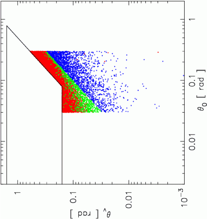
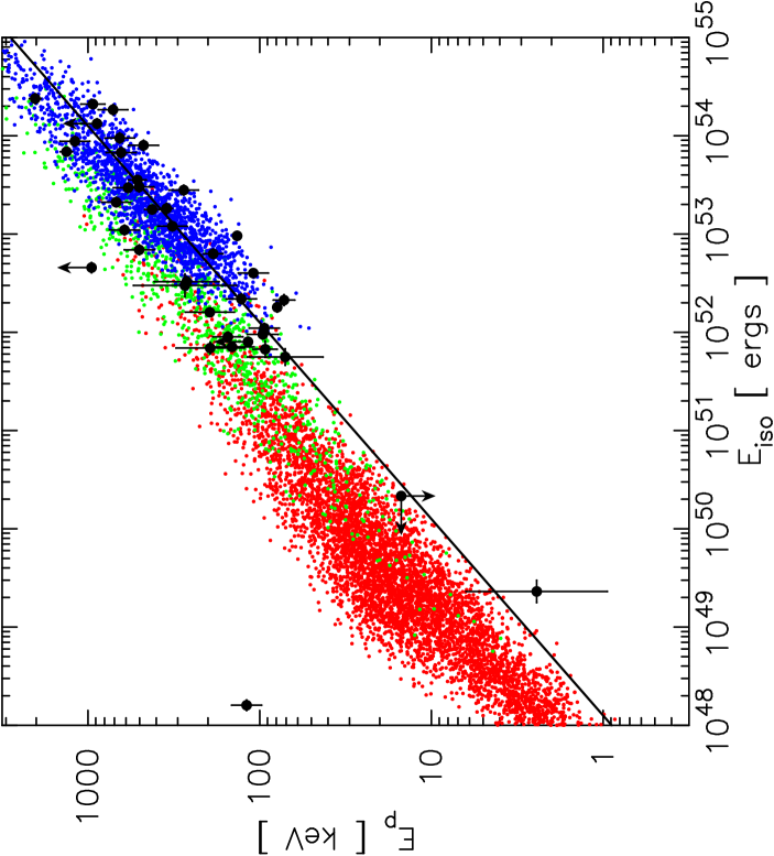
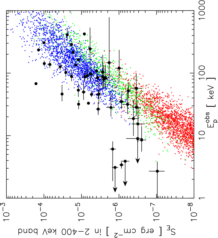
Figure 4.— Model Y04, which uses the parameters of Yamazaki, Ioka & Nakamura (2004a), where GRBs are seen on-jet and XRFs are explained by off-jet relativistic kinematics. Bursts detected on-jet (blue), off-jet (green) and non-detected bursts (red) are shown in the [$\theta_{0}$,$\theta_{\rm v}$]-plane (left), [$E_{\rm iso}$,$E_{\rm peak}$]-plane (center) and the [$E^{\rm obs}_{\rm peak}$,$S_{E}$(2-400 keV)]-plane (right), with observed data from BeppoSAX and HETE-2 overplotted.

The upper-right panel of Figure 4 shows that the standard $E_{\gamma}$ value and a narrow range of opening angles is sufficient to explain the population of classical GRBs. By construction, the on-jet events follow the $E_{\rm peak}\propto E_{\rm iso}^{1/2}$ relation. Off-jet emission from similar bursts viewed at much larger $\theta_{\rm v}$ accounts for the population of green off-jet points that lie above the $E_{\rm peak}\propto E_{\rm iso}^{1/2}$ relation. Off-jet events account for $34$% of the total detected bursts (see Table 1). For different values of $\theta_{\rm v}$, these bursts generally move along trajectories in the [$E_{\rm iso}$,$E_{\rm peak}$]-plane that have a flatter slope than the $E_{\rm peak}\propto E_{\rm iso}^{1/2}$ relation (see Figure 2). The observed off-jet bursts (green points) are consistent with only a few observed bursts, and for the most part, represent a population of events not seen by current instruments.

In particular, the middle and right panels of Figure 4 show that the HETE-2 XRFs are not easily explained as classical GRBs viewed off-jet, as this model posits. The two XRFs with known redshifts lie along the $E_{\rm peak}\propto E_{\rm iso}^{1/2}$ relation, and furthermore, the larger sample of HETE-2 XRFs without known redshifts do not fall in the region of the [$E^{\rm obs}_{\rm peak}$,$S_{\rm E}$]-plane expected for this model (they lie at lower, rather than higher, $E^{\rm obs}_{\rm peak}$ values for a given $S_{\rm E}$).

3.2. Top-Hat Variable Opening-Angle Jet Models

The next two models seek to explain both GRBs and XRFs by a wide distribution of jet opening-angles (see Lamb, Donaghy, & Graziani (2005) for more details and discussion). These models generate XRFs that obey the $E_{\rm peak}\propto E_{\rm iso}^{1/2}$ relation by extending the range of possible jet opening solid-angles to cover five orders of magnitude. Hence, XRFs that obey the $E_{\rm peak}\propto E_{\rm iso}^{1/2}$ relation are bursts that are seen on-jet, but have larger jet opening-angles. Here I add the presence of off-jet relativistic kinematics to this picture. These models generate a significant population of off-jet events, although increasing $\gamma$ reduces the fraction of off-jet bursts in the observed sample.

I draw $\Omega_{0}=2\pi(1-\cos\theta_{0})$ values from a power-law distribution given by $f_{0}\,d\Omega_{0}\propto\Omega_{0}^{-2}\,d\Omega_{0}$, defined from $2\pi$ to $2\pi\times 10^{-5}$ sr. $E^{\rm true}_{\gamma}$ is drawn from a narrow lognormal distribution centered on $1.2\times 10^{49}$ erg. The lower central point for the $E^{\rm true}_{\gamma}$ distribution is a requirement for including in a unified model those events with measured $E_{\rm iso}$ values that are smaller than the usual standard energy of $\sim 10^{51}$ ergs. I consider $\gamma=100$ (THVOA1, Figure 5) and $\gamma=300$ (THVOA2, Figure 6).

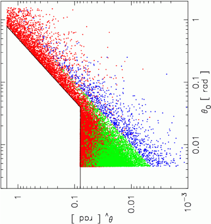
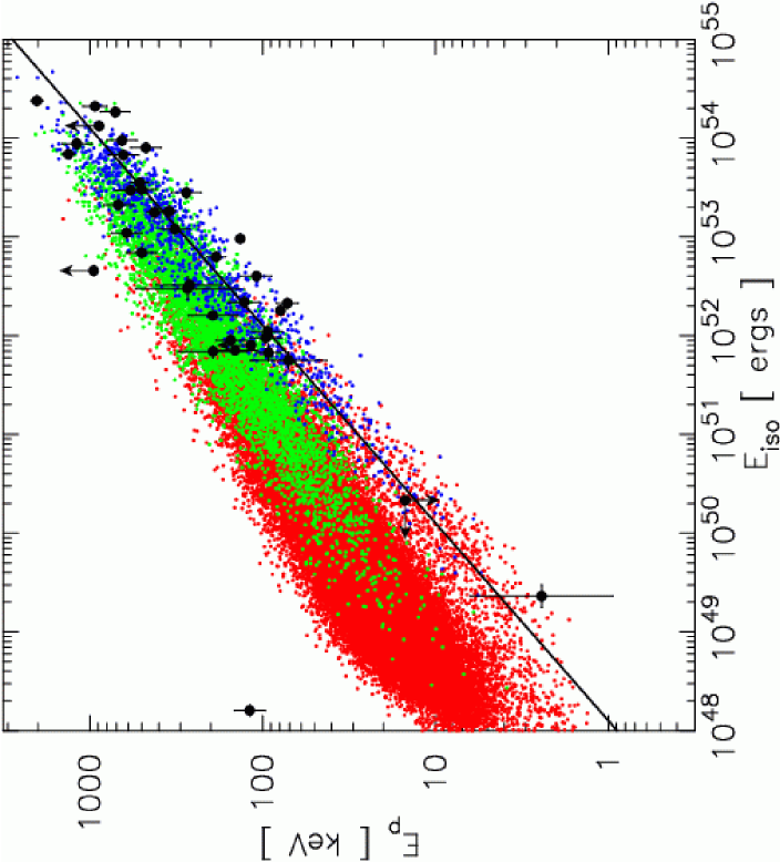
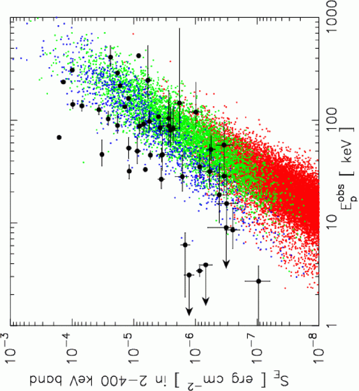
Figure 5.— THVOA1 model, which explains both GRBs and XRFs by a wide distribution of jet opening-angles, using $\gamma=100$. Bursts detected on-jet (blue), off-jet (green) and non-detected bursts (red) are shown in the [$\theta_{0}$,$\theta_{\rm v}$]-plane (left), [$E_{\rm iso}$,$E_{\rm peak}$]-plane (center) and the [$E^{\rm obs}_{\rm peak}$,$S_{E}$(2-400 keV)]-plane (right), with observed data from BeppoSAX and HETE-2 overplotted.

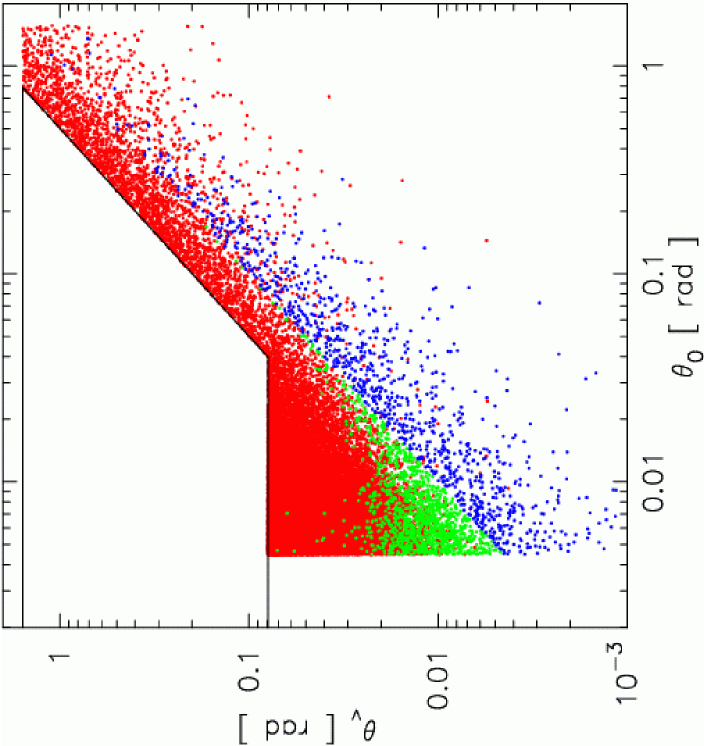
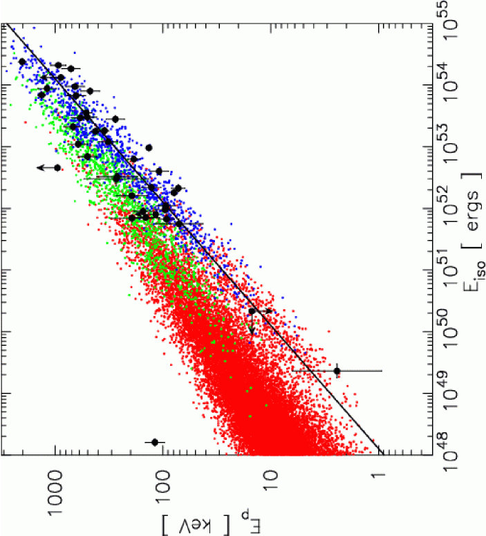
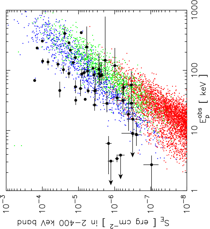
Figure 6.— THVOA2 model, which explains both GRBs and XRFs by a wide distribution of jet opening-angles, using $\gamma=300$. Bursts detected on-jet (blue), off-jet (green) and non-detected bursts (red) are shown in the [$\theta_{0}$,$\theta_{\rm v}$]-plane (left), [$E_{\rm iso}$,$E_{\rm peak}$]-plane (center) and the [$E^{\rm obs}_{\rm peak}$,$S_{E}$(2-400 keV)]-plane (right), with observed data from BeppoSAX and HETE-2 overplotted.

As can be seen from the upper-left panels of Figures 5 and 6, the relative importance of off-jet events increases for models with a population of very small opening-angles. This is mainly due to the fact that for constant $E_{\gamma}$, narrower jets will have larger $E_{\rm iso}$ values. Such bursts will be brighter and therefore detectable at larger $\theta_{\rm v}$. Narrow jets are also more likely to be viewed off-jet than wider jets. Finally, smaller values of $\theta_{0}$ give rise to trajectories in the [$E_{\rm iso}$,$E_{\rm peak}$]-plane that differ more conspicuously from the $E_{\rm peak}\propto E_{\rm iso}^{1/2}$ relation.

The large population of very small jet opening angles in these models also implies a much larger true burst rate than in model Y04. As Table 1 shows, for these two models the WXM will detect 1 out of 2570 and 6470 bursts respectively, as compared to 1 out of 150 bursts for the Y04 model.

For larger values of $\gamma$, the emission curves in Figure 1 drop off faster away from the edge of the jet. Comparing the upper-right panels of Figures 5 and 6 illustrates the fact that larger values of $\gamma$ reduce the percentage of off-jet events observed by the WXM, and consequently the percentage of bursts seen away from the $E_{\rm peak}\propto E_{\rm iso}^{1/2}$ relation. This population of events is fairly conspicuous in the $\gamma=100$ case ($83$% of detected bursts are off-jet events) and less so for $\gamma=300$ ($56$%).

Furthermore, this figure highlights the fact that observed XRFs are more easily explained by wide opening-angle jets than by off-jet emission. No matter the value of $\gamma$, observed XRFs inhabit different regions of the data planes than do off-jet events.

3.3. Models Matching the $E_{\rm peak}\propto E_{\gamma}^{\beta}$ Relation

Reproducing the $E_{\rm peak}\propto E_{\gamma}^{\beta}$ relation (Ghirlanda et al., 2004) is an important test of any jet model. Discovery of this relation post-dated Lamb, Donaghy, & Graziani (2005), and so was not addressed in that paper. Here I construct models that satisfy this relation, in addition to the constraints of the earlier models (for more details see Donaghy, Lamb, & Graziani (2005c)).

The $E_{\rm peak}\propto E_{\rm iso}^{1/2}$ and $E_{\rm peak}\propto E_{\gamma}^{\beta}$ relations can be mutually satisfied in the top-hat variable opening-angle jet model by imposing a relation between $\Omega_{0}$ and $E_{\gamma}$. The following expressions hold only for the on-jet events; the off-jet events behave differently. Combining Equations 7 and 8 with the definition

$$E_{\rm iso}=\frac{E_{\gamma}}{\Omega_{0}/2\pi}=\frac{E_{\gamma}}{1-\cos\theta_{0}},$$ (9)

I find

$$E_{\rm peak}=C_{A}\left(\frac{E_{\gamma}\cdot 2\pi}{E_{A}\cdot\Omega_{0}}\right)^{\alpha}=C_{G}\left(\frac{E_{\gamma}}{E_{G}}\right)^{\beta}$$ (10)

and solving for $\Omega_{0}$ gives the following expression

$$\Omega_{0}=2\pi(1-\cos\theta_{0})=2\pi\left(\frac{C_{A}}{C_{G}}\cdot\frac{E_{G}^{\beta}}{E_{A}^{\alpha}}\right)^{1/\alpha}E_{\gamma}^{(\alpha-\beta)/\alpha}.$$ (11)

I consider two different models in which $\Omega_{0}$ and $E^{\rm true}_{\gamma}$ are specified by imposing this relationship. The natural minimum value for the distribution of $E^{\rm true}_{\gamma}$ is the point $E^{*}$ at which $E_{\gamma}=E_{\rm iso}$, which is found to be

$$E^{*}=\left(\frac{C_{A}E_{G}^{\beta}}{C_{G}E_{A}^{\alpha}}\right)^{1/(\beta-\alpha)}.$$ (12)

Current parameters for the correlations give a value of $E^{*}=3\times 10^{44}$ ergs, which is well below current observational thresholds. Values of $E^{\rm true}_{\gamma}$ are generated by drawing from a power-law distribution that gives equal numbers of bursts per decade, and is defined from $E^{*}$ through a maximum value ($E^{\rm true}_{\gamma}=3.16\times 10^{51}$ ergs) that encompasses the largest observed $E_{\gamma}$ value ($E^{\rm inf}_{\gamma}=5.75\times 10^{51}$ ergs for GRB 990123). To avoid a sharp cutoff at the minimum and maximum values of $E_{\gamma}$, I include an additional smearing function in the simulated value of $E^{\rm true}_{\gamma}$ with a lognormal width of $0.3$ decades. $\Omega_{0}$ (and hence $\theta_{0}$) are found via Equation 11, and the rest of the simulations proceed as above. Results for $\gamma=100$ (GGL1) and $\gamma=300$ (GGL2) are shown in Figures 7 and 8, respectively.

Current data seems to indicate that the $E_{\rm peak}\propto E_{\gamma}^{\beta}$ relation has a narrower distribution about the best-fit line than does the $E_{\rm peak}\propto E_{\rm iso}^{1/2}$ relation (Ghirlanda et al., 2004). Adding a Gaussian smearing function to $C_{A}$, as was done in the above models, produces equal widths for both distributions. To broaden the $E_{\rm peak}\propto E_{\rm iso}^{1/2}$ relation, I introduce an additional Gaussian smearing function into the relation between $E_{\gamma}$ and $\Omega_{0}$. Equation 11 then becomes

$$\Omega_{0}=\frac{2\pi}{C_{\Omega}}\left(\frac{C_{A}}{C_{G}}\cdot\frac{E_{G}^{\beta}}{E_{A}^{\alpha}}\right)^{1/\alpha}E_{\gamma}^{(\alpha-\beta)/\alpha},$$ (13)

where $C_{\Omega}$ is centered on $1.0$ and has a lognormal width of $0.3$. Combined with the above value of the smearing in $C_{A}$, this approach and value of $C_{\Omega}$ gives good agreement with both observed distribution widths.

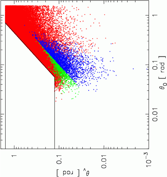
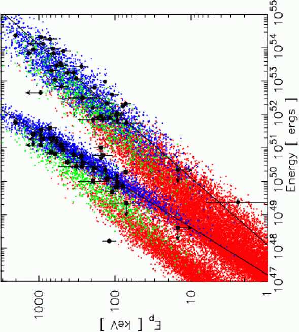
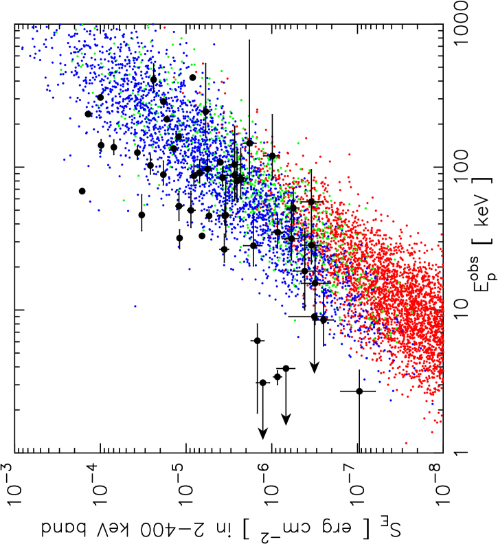
Figure 7.— GGL1 model, which picks parameters to match both the $E_{\rm peak}\propto E_{\rm iso}^{1/2}$ and $E_{\rm peak}\propto E_{\gamma}^{\beta}$ relations, using $\gamma=100$. Bursts detected on-jet (blue), off-jet (green) and non-detected bursts (red) are shown in the [$\theta_{0}$,$\theta_{\rm v}$]-plane (left), [$E$,$E_{\rm peak}$]-plane (center) and the [$E^{\rm obs}_{\rm peak}$,$S_{E}$(2-400 keV)]-plane (right), with observed data from BeppoSAX and HETE-2 overplotted.

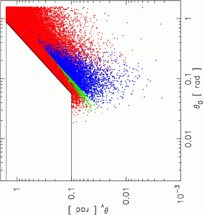
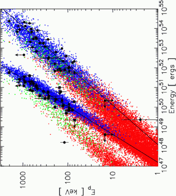
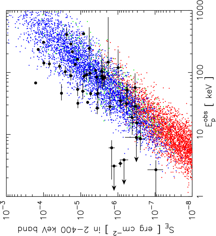
Figure 8.— GGL2 model, which picks parameters to match both the $E_{\rm peak}\propto E_{\rm iso}^{1/2}$ and $E_{\rm peak}\propto E_{\gamma}^{\beta}$ relations, using $\gamma=300$. Bursts detected on-jet (blue), off-jet (green) and non-detected bursts (red) are shown in the [$\theta_{0}$,$\theta_{\rm v}$]-plane (left), [$E$,$E_{\rm peak}$]-plane (center) and the [$E^{\rm obs}_{\rm peak}$,$S_{E}$(2-400 keV)]-plane (right), with observed data from BeppoSAX and HETE-2 overplotted.

An immediate consequence of the $\Omega_{0}$-$E_{\gamma}$ correlation is a lack of very small jet opening-angles and a narrower range of $\theta_{0}$ (compare the upper-right panels of Figures 6 and 8). The bursts observed off-jet lie closer to the $E_{\rm peak}\propto E_{\rm iso}^{1/2}$ relation than in models without the correlation (compare the upper-left panels of Figures 6 and 8). This is due to the narrower range of $\theta_{0}$ values mentioned above; larger $\theta_{0}$ values produce trajectories in the [$E_{\rm iso}$,$E_{\rm peak}$]-plane that closer approximate a $0.5$ power-law. The off-jet bursts also deviate further from the $E_{\rm peak}\propto E_{\gamma}^{\beta}$ relation than from the $E_{\rm peak}\propto E_{\rm iso}^{1/2}$ relation. This is due to that fact that, given an on-jet and an off-jet event that lie near each other on the $E_{\rm peak}\propto E_{\rm iso}^{1/2}$ relation, the off-jet event is more likely to have a smaller $\theta_{\rm br}$ than the on-jet event, thereby giving a smaller $E^{\rm inf}_{\gamma}$ value.

In comparison with the two THVOA models, these models exhibit much smaller true burst rates (1 detection for every 165 and 197 bursts, respectively) and smaller fractions of off-jet events ($26$% and $10$% of detected bursts, respectively). The additional Gaussian smearing function, $C_{\Omega}$, has the effect of blurring the clear separation of blue and green points along the $E_{\rm peak}\propto E_{\rm iso}^{1/2}$ relation (compare THVOA1 and GGL1), but not along the $E_{\rm peak}\propto E_{\gamma}^{\beta}$ relation in which $C_{\Omega}$ plays no role.

3.4. Models with $\Omega_{0}$-$\gamma$ Correlations

Finally, I investigate the effect of an additional correlation between $\Omega_{0}$ and $\gamma$. If narrower jets have larger bulk $\gamma$ values, this could reduce the importance of off-jet emission even further. The exact relationship between the bulk $\gamma$ of the material and the opening-angle of the jet is unknown. Extending the GGL models in the previous section, I consider a simple model (GCOR) in which $\gamma$ is given by $\gamma\propto\Omega_{0}^{-1}$. I fix the normalization by setting $\gamma=1000$ for the bursts with the narrowest jets.

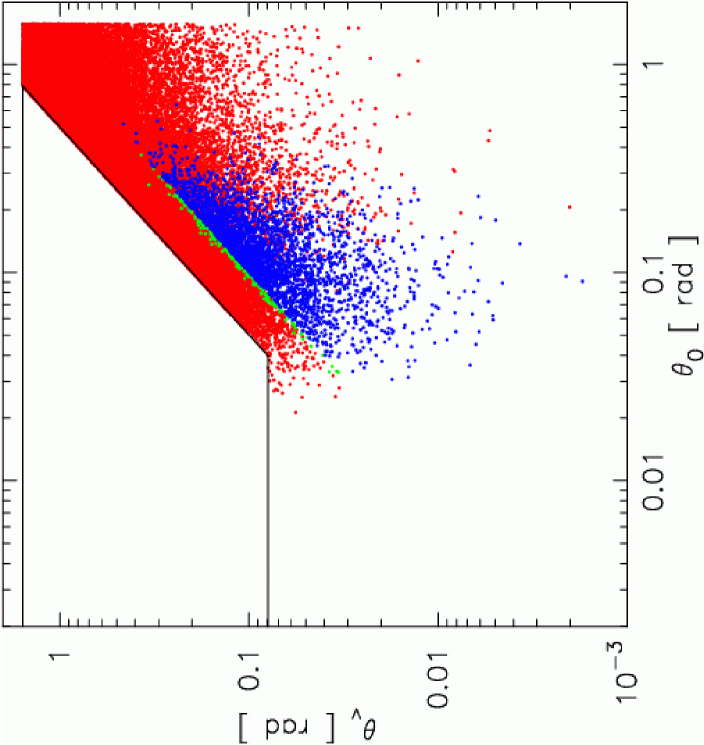
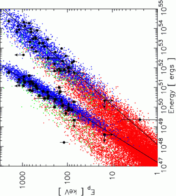
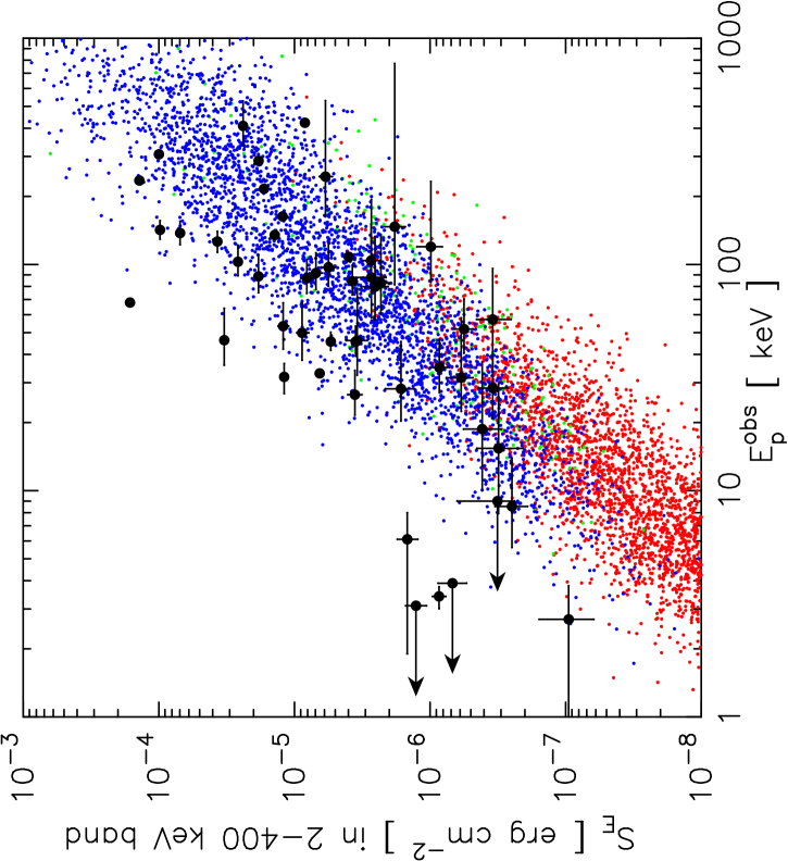
Figure 9.— Model GCOR where $\gamma\propto\Omega_{0}^{-1}$ and $\gamma=1000$ at the minimum value of $\Omega_{0}$. Bursts detected on-jet (blue), off-jet (green) and non-detected bursts (red) are shown in the [$\theta_{0}$,$\theta_{\rm v}$]-plane (left), [$E$,$E_{\rm peak}$]-plane (center) and the [$E^{\rm obs}_{\rm peak}$,$S_{E}$(2-400 keV)]-plane (right), with observed data from BeppoSAX and HETE-2 overplotted.

Figure 9 shows that imposing this correlation greatly reduces the percentage of bursts seen off-jet ($<7$% of detected bursts are seen off-jet). Physically this is due to a combination of several effects. It is more probable to observe narrow jets at viewing angles slightly outside the jet than inside the jet, yet for such narrow jets a large value of $\gamma$ ensures that the detectability of such slightly-off-jet bursts drops off very quickly with viewing angle. Broader jets may have smaller values of $\gamma$, but they are less likely to be observed off-jet.

4. Discussion

Table 1 summarizes the detected fractions and off-jet fractions for the six models. The detected fraction has direct implications for the total rate of GRBs. The ratio of the observed rate of Type Ic supernovae to the observed rate of GRBs is roughly $10^{5}$ (Lamb, 1999, 2000), and therefore the ratio of the observed rate of Type Ic supernovae to the true rate of GRBs is that value times the detected fraction for the model. Due to their very narrow jets, the THVOA models have the smallest detected fractions of the six models presented here. For the model THVOA2, GRBs may comprise an appreciable fraction of all observed Type Ic supernovae, but for all other models, the true rate of GRBs is much smaller than the observed supernova rate.

Model	Detected Fraction	Off-Jet Fraction
Y04	$0.00659=1/151.7$	$0.339$
THVOA1	$0.00039=1/2571.1$	$0.829$
THVOA2	$0.00015=1/6467.3$	$0.561$
GGL1	$0.00606=1/165.0$	$0.262$
GGL2	$0.00507=1/197.3$	$0.103$
GCOR	$0.00489=1/204.4$	$0.066$

Table 1Detection statistics for the six models presented in this paper. The second column shows the true rate of detection for all bursts in the model. Note that this is not the same as the percentage of bursts detected in the samples of $50,000$ due to the truncation described above. I correct for that truncation in calculating the detection fraction. The third column shows the fraction of all detected bursts that are seen off-jet.

In the figures above, I compare theoretical models employing the WXM detector threshold with data compiled from many instruments with varying detector sensitivities. To assess the effect of the detector thresholds in the simulations, I compare the predicted distributions of observed bursts for the two most successful models (GGL2 and GCOR) using the WXM instrument and using the GRBM instrument on BeppoSAX. For these two models, I compare the predicted distribution of observed bursts employing a given instrument threshold only with the data from that instrument.

Figure 10 shows that the higher triggering threshold for the GRBM instrument on BeppoSAX prevented that mission from promptly localizing the fainter, low-$E_{\rm peak}$ XRFs. In contrast, rapid HETE-2 localizations of XRFs have provided evidence that the $E_{\rm peak}\propto E_{\rm iso}^{1/2}$ relation extends to lower $E_{\rm peak}$ values, but HETE-2 has detected fewer high-$E_{\rm peak}$ bursts than BeppoSAX. Therefore, the models presented in this paper employing the WXM threshold are a good match for the full-range of observed GRB characteristics.

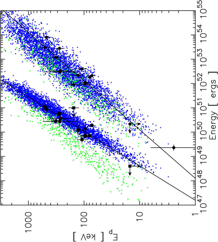
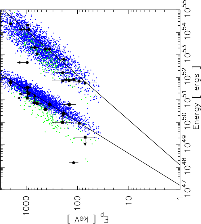
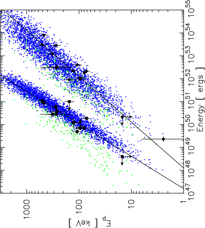
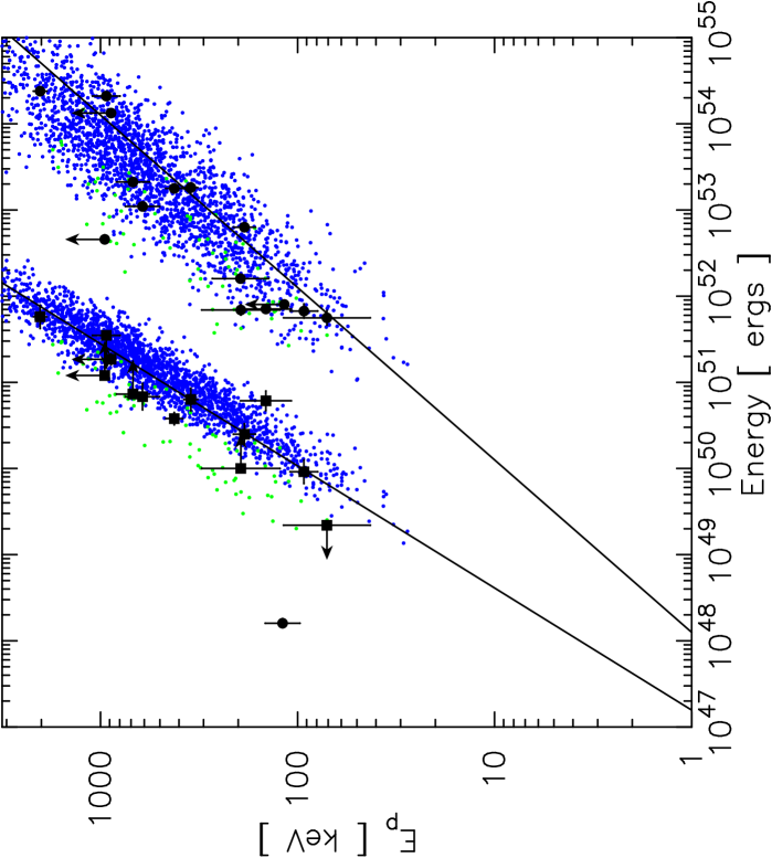
Figure 10.— The effect of different detector thresholds for two models, GGL2 (upper row) and GCOR (lower row). Bursts are shown in the [$E$,$E_{\rm peak}$]-plane, comparing models employing the WXM threshold against WXM data points (left column) and models employing the BeppoSAX threshold against BeppoSAX data points (right column).

Figures 11, 12 and 13 summarize the six models by comparing the observed data sets against the model cumulative distributions of $E_{\rm iso}$, $E_{\rm peak}$, $E^{\rm inf}_{\gamma}$, $\theta_{\rm br}$, $E^{\rm obs}_{\rm peak}$, and $S_{E}$(2-400 keV). Although a great deal of information is lost in projecting the 2-dimensional distributions from the above figures onto each axis separately, some useful information can still be obtained from these curves.

Figure 11 shows the cumulative distributions for $E_{\rm iso}$ and $E_{\rm peak}$, again separately comparing models using either the WXM or GRBM instrumental threshold with data obtained from that instrument. Due to the small size of the current datasets, the THVOA, GGL and GCOR models would not be judged as inconsistent with the data by the KS test. Model Y04 is here seen to over-produce brighter, high-$E_{\rm peak}$ events, and under-produce low-$E_{\rm peak}$ XRFs.

Figure 11.— The cumulative distribution in $E_{\rm iso}$ (left column) and $E_{\rm peak}$ (right column) for detected bursts in the six models explored in this paper. The upper row compares models employing the GRBM detector with data points observed by BeppoSAX. The lower row compares models employing the WXM detector with data points observed by HETE-2. The data used for the $E_{\rm peak}$ and $E_{\rm iso}$ distributions are the same as in Figure 3b, broken down by detector.

Figure 12 shows the cumulative distributions for $E^{\rm inf}_{\gamma}$ and $\theta_{\rm br}$, again separately comparing models using either the WXM or GRBM detector threshold with data obtained from that detector. This dataset is even sparser than that of Figure 11, but the figure does highlight the effect of rescaling the standard energy downward to $10^{49}$ ergs for the two THVOA models. The GGL and GCOR models avoid this problem by incorporating the $E_{\rm peak}\propto E_{\gamma}^{\beta}$ relation, and thereby avoid the large disparity with the $E^{\rm inf}_{\gamma}$ and $\theta_{\rm br}$ distributions seen for the THVOA models.

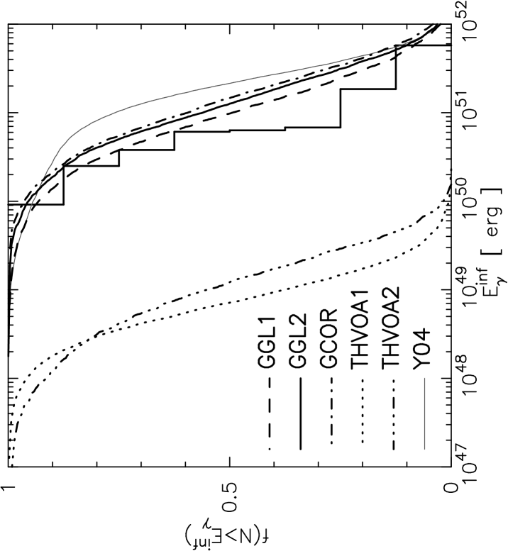
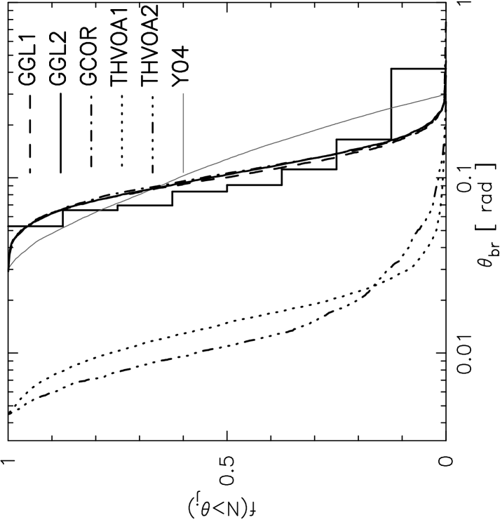
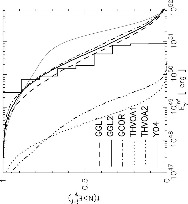
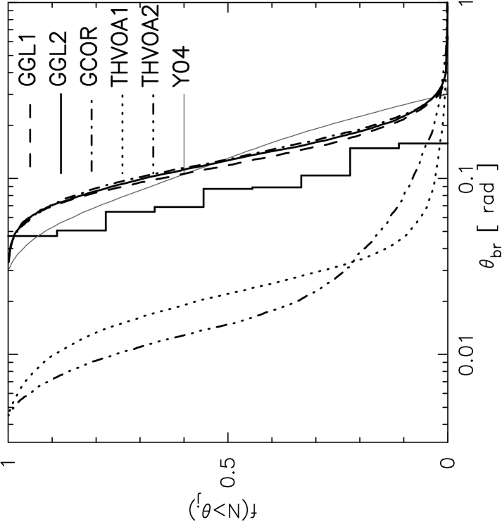
Figure 12.— The cumulative distribution in $E^{\rm inf}_{\gamma}$ (left column) and $\theta_{\rm br}$ (right column) for detected bursts in the six models explored in this paper. The upper row compares models employing the GRBM detector with data points observed by BeppoSAX. The lower row compares models employing the WXM detector with data points observed by HETE-2. The data used for the $E^{\rm inf}_{\gamma}$ distribution are the same as in Figure 3b, broken down by detector. The data used in the $\theta_{\rm br}$ distribution is the dataset from Ghirlanda et al. (2004).

Figure 13 shows the cumulative distributions for $E^{\rm obs}_{\rm peak}$ and $S_{E}$(2-400 keV), comparing models using the WXM detector threshold with the larger dataset of all bursts localized by HETE-2. Again, the THVOA, GGL and GCOR models are all reasonably consistent with the data. There is some hint that the GGL and GCOR models produce more bright, high-$E_{\rm peak}$ bursts than were seen by HETE-2, but this may be the result of trying to match both the BeppoSAX and HETE-2 populations with one model.

Figure 13.— The cumulative distribution in $E^{\rm obs}_{\rm peak}$ (left) and $S_{E}$(2-400 keV) (right) for detected bursts in the six models explored in this paper. These panels compare models employing the WXM detector with the larger dataset of all bursts localized by HETE-2. The data used for these distributions are taken from Sakamoto et al. (2005a) and Barraud et al. (2003).

To summarize, models GGL2 and GCOR are the most successful at matching the 2-dimensional distributions discussed above as well as the individual cumulative distributions. Model Y04, which seeks to explain XRFs as off-jet GRBs, is unable to match the distributions of observed XRFs. The THVOA models produce large numbers of detectable bursts away from the $E_{\rm peak}\propto E_{\rm iso}^{1/2}$ relation which are not seen in current datasets, and require a re-scaled standard energy of $10^{49}$ ergs, which is inconsistent with current afterglow theories (Panaitescu & Kumar, 2001).

5. Conclusions

Bursts with known redshifts have been found to obey the $E_{\rm peak}\propto E_{\rm iso}^{1/2}$ relation, and a large population of bursts away from this relation is not readily apparent in current datasets. In particular, the limited sample of XRFs with known redshift information is consistent with an extension of the $E_{\rm peak}\propto E_{\rm iso}^{1/2}$ relation to over 5 orders of magnitude in $E_{\rm iso}$. Liang, Dai & Wu (2004) found that the $E_{\rm peak}\propto E_{\rm iso}^{1/2}$ relation holds internally within a large sample of bright BATSE bursts without known redshift, perhaps indicating that the relation is a signature of the physics of the emission mechanism. However, recently some authors have argued that the $E_{\rm peak}\propto E_{\rm iso}^{1/2}$ relation may be an artifact of some unknown selection effect arising from the process of determining the burst redshift, and that $25$% (Nakar & Piran, 2004) to $88$% (Band & Preece, 2005) of the BATSE bursts may be inconsistent with the $E_{\rm peak}\propto E_{\rm iso}^{1/2}$ relation. However, these results are controversial (Ghirlanda et al., 2005a; Bosnjak et al., 2005; Lamb et al., 2005) and depend sensitively on the quality of the spectral fit that generates the $E^{\rm obs}_{\rm peak}$ parameter. I therefore regard the question of the percentage of BATSE bursts that are inconsistent with the $E_{\rm peak}\propto E_{\rm iso}^{1/2}$ relation to be an open one.

For low values of $\gamma$, top-hat variable opening-angle jet models predict a sizable population of detectable, off-jet bursts that lie away from the $E_{\rm peak}\propto E_{\rm iso}^{1/2}$ relation and that are not seen in current data sets. It may be that such bursts are in fact present in the BATSE catalog and form a population of bursts that do not obey the $E_{\rm peak}\propto E_{\rm iso}^{1/2}$ relation. On the other hand, if such a population is found not to exist, it implies that the bulk $\gamma$ of the jet is large ($\sim 300-1000$). For models that include the $E_{\rm peak}\propto E_{\gamma}^{\beta}$ relation, the off-jet burst population lies closer to the $E_{\rm peak}\propto E_{\rm iso}^{1/2}$ relation than for other models, but a similarly discrepant population of off-jet bursts is found to lie above the $E_{\rm peak}\propto E_{\gamma}^{\beta}$ relation, leading to similar conclusions.

Regardless of the size of the population of off-jet bursts, it seems unlikely that such a population can make up the bulk of the XRFs observed by HETE-2. The larger sample of HETE-2 bursts without redshift information contains XRFs which lie toward smaller $E^{\rm obs}_{\rm peak}$ values than is predicted by the off-jet emission model and hence are not easily explained as classical GRBs viewed off-jet. Models in which XRFs are the product of larger jet opening-angles seem to better match the observed distributions of XRF properties. This seems to match the evidence arising from X-ray afterglows of XRFs. Granot et al. (2005) calculated the afterglow light curves predicted by various models of burst emission seen off-jet. They find that a general feature of off-jet afterglows is an initial rising light-curve that peaks at about the jet break time and then declines rapidly, similar to an on-jet event. Afterglows with initially rising components have not been observed. In particular, XRFs with well-observed X-ray afterglows, for example XRF 020427 (Amati et al., 2004) and XRF 050215b (Sakamoto et al., 2005b), have afterglow light curves that join smoothly onto the end of the prompt emission and that show no evidence of a jet break for many days after the burst, implying large jet opening-angles.

It is straightforward to arrange for top-hat variable opening-angle jet models to match the empirical $E_{\rm peak}\propto E_{\gamma}^{\beta}$ relation, and such models also provide a natural explanation for XRFs. Figures 7 and 8 illustrate the consequences of adopting the correlation between $\Omega_{0}$ and $E^{\rm true}_{\gamma}$ that ensures that on-jet events obey the $E_{\rm peak}\propto E_{\gamma}^{\beta}$ relation. Most importantly, incorporating the $E_{\rm peak}\propto E_{\gamma}^{\beta}$ relation in the THVOA model removes two of the main drawbacks of the THVOA model presented in Lamb, Donaghy, & Graziani (2005). The requirement of very small ($\sim 2^{\circ}$) jet opening angles to explain the largest $E_{\rm iso}$ values was criticized (Stern, 2003) as being difficult to achieve in a hydrodynamic jet. The high end of the $E_{\rm iso}$ distribution is here explained by jets with moderate opening angles but larger $E_{\gamma}$ values. The need to re-scale the central value of $E^{\rm true}_{\gamma}$ downward to $\sim 10^{49}$ ergs to incorporate the XRFs in a unified model was criticized as being difficult to reconcile with afterglow models. The $E_{\rm peak}\propto E_{\gamma}^{\beta}$ relation naturally produces a range of $E_{\gamma}$ values that extends down into the XRF regime.

Matching the $E_{\rm peak}\propto E_{\gamma}^{\beta}$ relation also mitigates the problem of a large population of bursts seen away from the $E_{\rm peak}\propto E_{\rm iso}^{1/2}$ relation in the low $\gamma$ case. In these models the off-jet events hew more closely to the $E_{\rm peak}\propto E_{\rm iso}^{1/2}$ relation, but a similar problem arises in that these off-jet events are seen away from the $E_{\rm peak}\propto E_{\gamma}^{\beta}$ relation instead. A possible way out of this dilemma might be to impose a relationship whereby narrower jets have larger bulk $\gamma$ values and broader jets have smaller $\gamma$ values. Using a simple model where $\gamma\propto 1/\Omega_{0}$ results in a substantial reduction in the percentage of detected bursts seen off-jet.

Yamazaki, Ioka & Nakamura (2004b) have proposed a multiple subjet model for unifying short and long GRBs, X-ray-rich GRBs and XRFs. The model employs emission from multiple subjets (seen off-subjet) to explain X-ray-rich GRBs and XRFs. The authors performed Monte Carlo simulations for a universal multiple subjet model and find that the results are consistent with the $E_{\rm peak}\propto E_{\rm iso}^{1/2}$ relation, albeit with considerable scatter (see Figure 4 in Toma et al. (2005)).

There are two reasons why the multiple subjet model better satisfies the $E_{\rm peak}\propto E_{\rm iso}^{1/2}$ relation. First, the authors choose $\gamma=300$, which satisfies the constraint on $\gamma$ that I find above. The behavior of bursts viewed outside the envelope of subjets should approximate the top-hat models considered in this work. If the authors had adopted a lower value of $\gamma$, the model would have produced a large number of bursts that lie away from the $E_{\rm peak}\propto E_{\rm iso}^{1/2}$ relation; i.e., they would have encountered the same problems as those of model THVOA1. Second, since $\gamma=300$, the spectrum for each line of sight is dominated by that of the closest subjet, and since there are many subjets, each line of sight lies very close to at least one subjet, mitigating the effects of relativistic kinematics produced by viewing a subjet well off the jet.

Finally, Toma et al. (2005) find that for values of $\gamma$ lower than $300$, the ratio between GRBs, X-ray-rich GRBs and XRFs becomes highly skewed toward hard GRBs, in contradiction with the HETE-2 results. Thus, all of the results in Toma et al. (2005) support the requirement I find in this paper that large gamma values are needed in order to match the observed data for XRFs, X-ray-rich GRBs, and GRBs.

Off-jet relativistic kinematics will be important in non-uniform jets as well as in top-hat jets. Models employing Gaussian (Zhang et al., 2004) or Fisher-shaped (Donaghy, Lamb, & Graziani, 2005a) jets rely on the exponential fall off of the emissivity with viewing angle to match the wide spread of observed burst quantities. By including off-jet emission in these models, the exponential fall off will be dominated at some angle by the power-law fall off due to relativistic kinematics, thereby broadening the emissivity distribution and reducing the range of generated $E_{\rm iso}$ values. Graziani et al. (2005) showed that different underlying burst profiles may have radically different observational distributions. We hope to use population synthesis Monte Carlo simulations to further explore these models in future work.

In conclusion, off-jet emission from collimated GRB outflows should exist simply as a consequence of relativistic kinematics. Monte Carlo population synthesis simulations of top-hat shaped variable opening-angle jet models predict a large population of off-jet bursts that are observable and that lie away from the $E_{\rm peak}\propto E_{\rm iso}^{1/2}$ and $E_{\rm peak}\propto E_{\gamma}^{\beta}$ relations. Such off-jet events are not apparent in current datasets. These discrepancies can be removed if $\gamma>300$ for all bursts or if there is a strong inverse correlation between $\gamma$ and $\Omega_{0}$. The simulations show that XRFs seen by HETE-2 and BeppoSAX cannot be easily explained as classical GRBs viewed off-jet, and are more naturally explained as jets with large opening-angles.

References

- Amati et al. (2002) Amati, L., et al. 2002, A&A, 390, 81
- Amati et al. (2004) Amati, L., et al. 2004, A&A, 426, 415
- Band et al. (1993) Band, D. L. et al. 1993, ApJ, 413, 281
- Band (2003) Band, D. L. 2003, ApJ, 588, 945
- Band & Preece (2005) Band, D. L. & Preece, R. D. 2005, ApJ, 627, 319
- Barraud et al. (2003) Barraud, C., et al. 2003, A&A, 400, 1021
- Bloom et al. (2003) Bloom, J., Frail, D. A., & Kulkarni, S. R. 2003, ApJ, 588, 945
- Bosnjak et al. (2005) Bosnjak, Z., et al. 2005, MNRAS, submitted (astro-ph/0502185)
- Donaghy (2005a) Donaghy, T. Q. 2005a, Il Nuovo Cimento, 28C, 407
- Donaghy, Lamb, & Graziani (2005a) Donaghy, T. Q., Lamb, D. Q., & Graziani, C. 2005a, Il Nuovo Cimento, 28C, 403
- Donaghy, Lamb, & Graziani (2005b) Donaghy, T. Q., Lamb, D. Q., & Graziani, C. 2005b, ApJ, submitted
- Donaghy, Lamb, & Graziani (2005c) Donaghy, T. Q., Lamb, D. Q., & Graziani, C. 2005c, ApJ, submitted
- Frail et al. (2001) Frail, D., et al. 2001, ApJ, 562, L55
- Friedman & Bloom (2004) Friedman, A. S. & Bloom, J. S. 2004, ApJ, 627, 1
- Ghirlanda et al. (2004) Ghirlanda, G., Ghisellini, G. & Lazzati, D. 2004, ApJ, 616, 331
- Ghirlanda et al. (2005a) Ghirlanda, G., Ghisellini, G., & Firmani, C. 2005a, MNRAS, 361, L10
- Ghirlanda et al. (2005b) Ghirlanda, G., Ghisellini, G., Lazzati, D. & Firmani, C. 2005b, Il Nuovo Cimento, 28C, 303
- Golenetskii et al. (2005a) Golenetskii, S., et al. 2005a, GCN Circ 3179, http://gcn.gsfc.nasa.gov/gcn/gcn3/3179.gcn3
- Golenetskii et al. (2005b) Golenetskii, S., et al. 2005b, GCN Circ 3473, http://gcn.gsfc.nasa.gov/gcn/gcn3/3473.gcn3
- Golenetskii et al. (2005c) Golenetskii, S., et al. 2005c, GCN Circ 3518, http://gcn.gsfc.nasa.gov/gcn/gcn3/3518.gcn3
- Granot et al. (2005) Granot, J., Ramirez-Ruiz, E. & Perna, R. 2005, ApJ, 630, 1003
- Graziani et al. (2005) Graziani, C., Donaghy, T. Q., & Lamb, D. Q. 2005, ApJ, in press (astro-ph/0505623)
- Harrison et al. (1999) Harrison, F. A., et al. 1999, ApJ, 559, 123
- Heise et al. (2001) Heise, J., in’t Zand, J., Kippen, R. M., & Woods, P. M., in Proc. 2nd Rome Workshop: Gamma-Ray Bursts in the Afterglow Era, eds. E. Costa, F. Frontera, J. Hjorth (Berlin: Springer-Verlag), 16
- Ioka & Nakamura (2001) Ioka K. & Nakamura T. 2001, ApJ, 554, L163
- Kippen et al. (2001) Kippen, R. M., Woods, P. M., Heise, J., in’t Zand, J., Briggs, M.S., & Preece, R. D. 2003, in AIP Conf. Proc. 662, Gamma-Ray Burst and Afterglow Astronomy, ed. G. R. Ricker & R. K. Vanderspek (New York: AIP), 244
- Kulkarni et al. (1998) Kulkarni, S. R., et al. 1998, Nature, 393, 35
- Kulkarni et al. (1999) Kulkarni, S. R., et al. 1999, Nature, 398, 389
- Lamb (1999) Lamb, D. Q. 1999, A&AS, 138, 607
- Lamb (2000) Lamb, D. Q. 2000, Phys. Rep., 333, 505
- Lamb, Donaghy, & Graziani (2005) Lamb, D. Q., Donaghy, T. Q., & Graziani, C. 2004, ApJ, 620, 355
- Lamb et al. (2005) Lamb, D. Q., et al. 2005, ApJ, submitted
- Liang, Dai & Wu (2004) Liang, E. W., Dai, Z. G., & Wu, X. F. 2004, ApJ, 606, L29
- Lloyd-Ronning et al. (2000) Lloyd-Ronning, N., Petrosian, V., & Mallozzi, R. S. 2000, ApJ, 534, 227
- Nakar & Piran (2004) Nakar, E. & Piran, T. 2004, ApJ, submitted (astro-ph/0412232)
- Panaitescu & Kumar (2001) Panaitescu, A. & Kumar, P. 2001, ApJ, 560, L49
- Rhoads (1997) Rhoads, J. E. 1997, ApJ, 478, L1
- Ricker et al. (2001) Ricker, G. R., et al. 2003, in AIP Conf. Proc. 662, Gamma-Ray Burst and Afterglow Astronomy, ed. G. R. Ricker & R. K. Vanderspek (New York: AIP), 3
- Rowan-Robinson (2001) Rowan-Robinson M. 2001, ApJ, 549, 745
- Sakamoto et al. (2004) Sakamoto, T., et al. 2004, ApJ, 602, 875
- Sakamoto et al. (2005a) Sakamoto, T., et al. 2005a, ApJ, 629, 311
- Sakamoto et al. (2005b) Sakamoto, T., et al. 2005b, ApJ, submitted
- Sari, Piran & Halpern (1999) Sari, R., Piran, T., Halpern, J. P. 1999, ApJ, 519, L17
- Stern (2003) Stern, B. E. 2003, MNRAS, 345, 590
- Toma et al. (2005) Toma, K., Yamazaki, R., & Nakamura T. 2005, ApJ, 635, 481