Filtration of atmospheric noise in narrow-field astrometry with very large telescopes

This paper presents a non-classic approach to narrow field astrometry that offers a significant improvement over conventional techniques due to enhanced reduction of atmospheric image motion. The method is based on two key elements: apodization of the entrance pupil and the enhanced virtual symmetry of reference stars. Symmetrization is implemented by setting special weights to each reference star. Thus a reference field itself forms a virtual net filter that effectively attenuates the image motion spectrum. Atmospheric positional error was found to follow a power dependency $\Delta\sim R^{k\mu/2}D^{-k/2+1/3}$ on angular field size $R$ and aperture $D$; here $k$ is some optional even integer $2\leq k\leq\sqrt{8N+1}-1$ limited by a number $N$ of reference stars, and $\mu\leq 1$ is a term dependent on $k$ and the magnitude and sky star distribution in the field. As compared to conventional techniques for which $k=2$, the improvement in accuracy increases by some orders. Limitations to astrometric performance of monopupil large ground-based telescopes are estimated. The total atmospheric and photon noise for at a 10 m telescope at good $0.4^{\prime\prime}$ seeing was found to be, depending on sky star density, 10 to 60 $\mu$as per 10 min exposure in R band. For a 100 m telescope and FWHM=0.1^′′ (low-order adaptive optics corrections) the potential accuracy is 0.2 to 2 $\mu$as.

1 Introduction

Atmospheric turbulence affects astronomical observations with respect to both image quality degradation and random image motion. With improvement of image detectors the second source of errors has become dominant in astrometric measurements. The very slow progress in overcoming atmospheric errors finally turned to development of high-accurate astrometry from space missions. The first successful Hipparcos mission yielded data with an accuracy of 1 mas, the GAIA project (Perryman et all. 2001) is aimed at 10 $\mu$as accuracy level.

The most promising direction of optical ground-based astrometry is now related to the infrared long-baseline interferometers; the atmospheric limit for this kind of instruments is about 10 $\mu$as (Shao & Colavita 1992; Paresce et all. 2002). Astrometry with monopupil long-focus telescopes is limited by much larger $\Delta\sim 1$ mas atmospheric error, which was confirmed by numerous experimental and theoretical data. Thus, Gatewood (1987), on the basis of measurements with the Multichannel Astrometric Photometer ($D=0.76$ m), derived $\Delta\simeq 3$ mas/hr with a reference frame of $10-20^{\prime}$. Using the same data, Han (1989) suggested a model of a image motion power spectrum according to which the distance between a $1^{\prime}$ separated double star can be measured with an accuracy of $\simeq 1$ mas/1hr. The best precision of 150 $\mu$as/hr ever obtained with ground-based telescopes was demonstrated by Pravdo & Shaklan (1996) with the 5-m Palomar telescope in a field of 90 arcsec.

A theoretical aspect of the image motion problem was studied by Lindegren (1980) who derived analytical expressions for relative image motion of a double star. For very narrow fields, $\Delta^{2}\sim(\rho h)^{2}D^{-4/3}T^{-1}$ demonstrated a rather weak power dependency of the variance of image motion $\Delta^{2}$ on the double star angular separation $\rho$, objective diameter $D$ and exposure $T$ ($h$ is the turbulent layer height). The above dependence shows that an improvement of $\Delta$ from 1 mas to say 10 $\mu$as will require unrealistically large $D$ and $T$, unless $\rho$ is limited to uselessly small angles. The situation is somewhat better when a very dense star field is used as a reference. For circular star samples of a radius $\rho$ the dependency becomes $\Delta^{2}\sim(\rho h)^{8/3}D^{-2}T^{-1}$ which is a factor $(\rho h/D)^{2/3}$ better than that valid for a single reference star. Lazorenko (2002a), making allowance for the second order term of the random phase fluctuations over the pupil, has proved that the dependency is $\Delta^{2}\sim(\rho h)^{11/3}D^{-3}T^{-1}$, or a factor $\rho h/D$ still stronger. He also suggested a symmetrizing procedure by means of which any arbitrary distributed sample of stars can be utilized as a virtually symmetric reference frame.

Nevertheless even the use of symmetric (or symmetrized) reference fields not can provide accuracies like those expected from interferometric and/or space mission techniques. Thus, Lazorenko (2002a), considering a 10 m telescope, $1^{\prime}$ diameter reference frame and all the turbulence concentrated at 2.8 km height, found that atmospheric noise is 5 $\mu$as/hr at moderate seeing. Scaling this data to more realistic effective heights of 14 – 17 km yields $\Delta=120$ – 300 $\mu$as/hr, which is the limit of this technique. An efficient solution of the problem suggested in the current paper is based on enhanced symmetrization of reference fields, which is an improved version of the former procedure (Lazorenko 2002a). This new approach allows a much better filtration of random wave-front distortions, reducing atmospheric noise to 1–10 $\mu$as/hr with a 10 m aperture.

This paper presents the analysis of atmospheric limits to astrometric performance of one-aperture telescopes. We emphasise the use of very large 10 – 100 m telescopes since we want to obtain limiting estimates of ground-based astrometry. Astrophysical drives and possible applications for microarcsecond astrometry are not discussed here although they were considered in some papers (Perryman et al. 2001; Pravdo & Shaklan 1996; Paresce et al. 2002). In Section 2 we describe a model of a differential image motion spectrum. The image motion spectrum filtration described in Section 3 is based on two key elements: apodization of the entrance pupil (Section 4) and the enhanced virtual symmetry of reference groups (Section 5). In Section 6 we consider asymptotic properties of high-order symmetry dense reference fields and in Section 7 we discuss modifications of plate reductions necessary to implement the new technique. Estimates of the image motion error integrated over the atmosphere are given in Section 8. Astrometric performance of very large telescopes under assumption of a two-component error budget is analyzed in Section 9.

2 A model of differential image motion power spectrum

Atmospheric random motion of the star image centroid is caused by turbulence which is known to be concentrated in a limited number of thin atmospheric layers. Each layer is described by its height $h$ above the ground, a thickness $\Delta h$ which is typically 10 – 100 m, rarely up to 800 m (e.g. Barletti et al. 1977; Redfern 1991; Vinnichenko et al. 1976) and a refractive-index structure constant $C^{2}_{n}$. Turbulent motion in each layer is isotropic in horizontal directions, and refractive-index fluctuations are described by the structure function $D_{n}({\bf r})=C^{2}_{n}r^{p}$, where $\bf r$ is a vector connecting two points in a 2-D layer’s plane, and $p$ is a constant. Some experimental and theoretical studies discussed by Lazorenko (2002a) testify that $p$ is to be considered as a variable term with a typical range of variations 1/2 – 2/3 which at some particular atmospheric conditions is widened from -1/3 to +1. In the present study, for the sake of universality of the derived equations, this quantity is considered as a variable, but numerical estimates are made with $p=2/3$ only.

Due to the small thickness of layers $\Delta h\ll h$, the each one is considered as a thin horizontal phase screen that produces random phase distortions of the light wave front. A plane wave that crosses the screen thus gains some random phase $\phi(x,y)$ where $x,y$ are Cartesian coordinates in the phase screen plane. Given the assumption of homogeneity and isotropy of turbulence (at least in a horizontal plane), the power spectral density of a phase is a function

$$\hat{F}_{\phi}(q)=c_{\phi}q^{-p-3}$$ (1)

of a circular spatial frequency $q$. Here $c_{\phi}$ is a factor accounting for turbulence strength. In case of the Kolmogorov turbulence, $c_{\phi}$ is related to $C^{2}_{n}$ via the expression (Tatarsky 1961)

$$c_{\phi}=0.033(2\pi/\lambda)^{2}(2\pi)^{-2/3}C^{2}_{n}\Delta h$$ (2)

where $\lambda$ is wavelength.

Perturbations of a light phase $\phi(x,y)$ lead to random displacements $\zeta$ of star image centroids in the focal plane. The magnitude of $\zeta$ measured in some arbitrary direction $\bf{r^{\prime}}$ is proportional to the gradient of the phase $\partial\phi(x,y)/\partial\bf{r^{\prime}}$ averaged over the screen section involved in image formation. For the instant exposure $T=0$ it is a circular area of a diameter $D$ equal to the telescope diameter and centered at the point $\bf r$ where the phase screen is crossed by light beams passing from the star to the centre of the telescope pupil. A quantity $\zeta$ as a function of $\bf r$ vector is given by the convolution (Martin 1987; Conan et al. 1995)

$$\zeta({\bf r})=\frac{\lambda}{2\pi}\frac{\partial\phi({\bf r})}{\partial{\bf r^{\prime}}}\ast\frac{P({\bf r})}{\sigma}$$ (3)

where $P({\bf r})$ is the entrance pupil function that determines optical transmission of the objective and

$$\sigma=\int\int P({\bf r})\,d{\bf r}$$ (4)

is the effective area of the entrance pupil. For a classical fully transparent monopupil

$$P({\bf r})=\left\{\begin{array}[]{ll}1,&r\leq D/2\\ 0,&r>D/2\end{array}\right.$$ (5)

At finite exposure $T>0$, the wind-induced motion of a phase screen with the wind velocity $V$ is to be taken into consideration since it causes extra averaging of phase fluctuations along a straight line of length $VT$. This effect is described by convolution of the function (3) with a rectangular function

$$\mbox{rect}(z)=\left\{\begin{array}[]{ll}(VT)^{-1},&z\leq VT/2\\ 0,&z>VT/2\end{array}\right.$$ (6)

where $z$ is measured along the wind direction which forms some angle $\varepsilon$ with the $x$-axis.

Figure 1: Geometric elements specifying a star group (circles) projection on a phase screen

In differential astrometry the position of the target object is measured with respect to some $N$ reference stars. Let us consider a geometry of a stellar group in projection on the phase screen displayed in Fig.1. The points B_i, $i=1\ldots N$ represent reference stars, the target star projection B₀ is given by the vector ${\bf r}$. Cartesian coordinates $x_{i}$, $y_{i}$ of stars are equal to their standard coordinates scaled to the layer height $h$. In polar coordinates, the distribution of points B_i is given by their linear separations from the target $s_{i}=h\rho_{i}$ where $\rho_{i}$ is $i$-th star angular separation from the target, by positional angles $\psi_{i}$ measured with respect to the $x$-axis and by distances $s_{ij}=\sqrt{s_{i}^{2}+s_{j}^{2}-2s_{i}s_{j}\cos(\psi_{i}-\psi_{j})}$ between the two points B_i and B_j.

Differential displacement of star images $\Delta\zeta$ is obviously equal to the difference of $\zeta({\bf r})$ function values taken at points B₀ and B_i. In the trivial case of one reference star B₁, the differential displacement is $\Delta\zeta({\bf r})=\zeta({\bf r})-\zeta({\bf r+s}_{1})=\zeta({\bf r})\ast\tilde{Q}({\bf r})$ where

$$\tilde{Q}({\bf r})=\delta({\bf r})-\delta({\bf r+s}_{1})$$ (7)

is a difference operator. For multi-star reference frames the form of the function (7) is specified by distribution of reference stars which we include by using designation $\tilde{Q}({\bf r,s})$.

Taking into account the above effects, we come to a common expression

$$\Delta\zeta({\bf r})=\frac{\lambda}{2\pi}\frac{\partial\phi({\bf r})}{\partial{\bf r^{\prime}}}\ast\mbox{rect}({\bf r})\ast P({\bf r})/\sigma\ast\tilde{Q}({\bf r,s})$$ (8)

inherent to the differential technique.

Now it is useful to proceed to the analysis in the frequency domain where the power spectral density $F_{\zeta}(q,\varphi)$ of the quantity $\Delta\zeta$ is expressed as a product of four squared Fourier transforms ${\mathcal{F}}{}$ of functions convolved in (8) and the power spectrum (1). In the polar coordinates $q$, $\varphi$

$$\begin{array}[]{ll}F_{\zeta}(q,\varphi)=&[\lambda/(2\pi)]^{2}{\mathcal{F}}^{2}\left\{\frac{\partial}{\partial{\bf r^{\prime}}}\right\}{\mathcal{F}}^{2}\left\{\frac{P}{\sigma}\right\}{\mathcal{F}}^{2}\{\mbox{rect}\}\\ &\times{\mathcal{F}}^{2}\{\tilde{Q}\}F_{\phi}(q)\\ \end{array}$$ (9)

It is known that ${\mathcal{F}}^{2}\{\partial/\partial{\bf r^{\prime}}\}=[2\pi q\mbox{cos}(\varphi-\theta)]^{2}$ and ${\mathcal{F}}^{2}\{\mbox{rect}\}=\mbox{sinc}^{2}[\pi VTq\mbox{cos}(\varphi-\varepsilon)]$ where $\theta$ is the angle formed by the vector ${\bf r^{\prime}}$ and $x$-axis and sinc$(z)=\sin(z)/z$ (e.g. Martin 1987; Lazorenko 2002a). Angular parameters $\varepsilon$ (the wind direction) and $\theta$ (direction of image motion measurements) present in the above expressions introduce anisotropic effects (Lazorenko 2002a), which makes the analysis rather complicated and requires a special discussion. However, there are some reasons permitting us to perform averaging of Eq.(9) over $\varepsilon$ and $\theta$. With respect to $\theta$, this procedure is justified by the fact that, normally, the image motion variance is defined as its mean value measured along the $x$ and $y$ axes, hence ${\mathcal{F}}^{2}\{\partial/\partial{\bf r^{\prime}}\}=2\pi^{2}q^{2}$. Averaging over another angle $\varepsilon$ is related to variations of the wind direction in the vertical profile of turbulence and to its temporal variability during the exposure in a single layer. Numerical estimates (Lazorenko 2002b) show that even small $\pm 5{\degr}$ variations in the wind direction cause an effect very similar to a complete averaging over 0–2$\pi$ range. The averaging leads to expression (Lazorenko 2002a) ${\mathcal{F}}^{2}\{\mbox{rect}\}=(\pi VTq)^{-1}$ valid for long exposures $T\gg D/V$. Finally, note that due to the forthcoming integration in the frequency plane, the angular-dependent function ${\mathcal{F}}^{2}\{\tilde{Q}\}$ in Eq.(9) can be substituted by its average

$$Q(q)=(2\pi)^{-1}\int_{0}^{2\pi}{\mathcal{F}}^{2}\{\tilde{Q}({\bf r,s})\}d\varphi$$ (10)

which is the filter induced by the reference star field. Then Eq.(9) takes the form

$$F_{\zeta}(q)=\frac{\lambda^{2}c_{\phi}}{2\pi VT}q^{-2-p}Y(q)Q(q)$$ (11)

where $Y(q)={\mathcal{F}}^{2}\{P/\sigma\}$ is the filter-function of the entrance pupil. Integration of the power density (11) over $q$ yields the variance of differential image motion

$$\Delta^{2}=\frac{\lambda^{2}c_{\phi}}{VT}\int_{0}^{\infty}Y(q)Q(q)q^{-1-p}\,dq$$ (12)

3 Image motion power spectrum attenuation

A concept of image motion variance (12) reduction takes advantage of the dependence of the power spectrum $F_{\zeta}(q)$ on filter $Y(q)$ and $Q(q)$ shape which generally can be corrected. To explain the concept of the method consider a classic example of double star observations with a filled monopupil (5) when functions $Y(q)$ and $Q(q)$ are given by expressions (e.g. Lazorenko 2002a)

$$\begin{array}[]{l}Y(q)=[2J_{1}(\pi Dq)/(\pi Dq)]^{2}\\ Q(q)=2[1-J_{0}(2\pi qs_{1})],\\ \end{array}$$ (13)

where $J_{m}$ are Bessel functions of the order $m$. In this study we suggest some improved modifications of filters (13) for better filtration of turbulent phase distortions. For this purpose we require that: 1) the low-pass filter $Y(q)$ is fast decreasing at frequencies longer than $D^{-1}$, and 2) the high-pass filter $Q(q)$ has very low response at short frequencies. A useful approximation of filter shapes is given by quasi-rectangular functions with flat peaks and drop-down segments:

$$\begin{array}[]{l}Y(q)=\left\{\begin{array}[]{ll}1,&\pi Dq\leq q_{0}\\ E_{\nu}(Dq/2)^{-\nu},&\pi Dq>q_{0}\\ \end{array}\right.\\ Q(q)=\left\{\begin{array}[]{ll}H_{k}(Sq)^{k},&\pi Sq\leq 1\\ Q_{\infty},&\pi Sq>1\\ \end{array}\right.\\ \end{array}$$ (14)

Here the terms $\nu$ and $k$ are the most important model parameters since they determine the asymptotic behaviour of filters; $E_{\nu}$, $H_{k}$ and $Q_{\infty}$ are quasi-constant terms, approximately independent of $\nu$ and $k$; $q_{0}$ specifies the filter $Y(q)$ nucleus width; $S$ is the effective linear size of the stellar group projection onto the phase screen.

In terms of this model, a very narrow field regime of observations is defined by a nonoverlapping position of $Q(q)$ and $Y(q)$ nuclei: $S\ll D/q_{0}$. With an approximation $q_{0}\approx 2$ following from Eq.(18) it is simply $S\ll D/2$.

Classic filters (13) are described by parameters $\nu=3$ and $k=2$.

Figure 2: Combined filter $Y(q)Q(q)$ response at $D/S=17.2$ for the two configurations of Table 2: ”a” (upper curve) – double star, $k=2$, $\nu=3$; and ”g” (lower curve) – at $k=8$, $\nu=9$

A qualitative demonstration of the current concept of enhanced image motion filtration requires using results from the next Sections 4–5. In Fig.2 we display the combined filtering effect of the product $Y(q)Q(q)$ for a double star observation ($k=2$, $\nu=3$, upper curve) which should be compared with that expected for improved parameters $\nu=9$ and $k=8$ (lower curve). The functions plotted refer to a $D=100$ m telescope, a single turbulent layer at $h=20$ km and star reference groups ”a” and ”g” of equal effective linear size $S=5.82$ m (Table 2). The much lower filter response in the second case ensures the essential reduction of the differential image motion spectrum and $\Delta^{2}$.

With the model (14), and the assumption of very narrow fields $S\ll D/2$, the value of $\Delta^{2}$ defined by the integral (12) is given by a two component sum

$$\Delta^{2}=[c_{1}(2S/D)^{k}+c_{2}(2S/D)^{\nu+p}]{(D/2)}^{p}{\pi}^{\nu-k+p}$$ (15)

where $c_{1}$ and $c_{2}$ are some slow functions of the model parameters. Under condition $k<\nu+p$, the first component prevails resulting in a power law $\Delta^{2}={(2S/D)}^{k}D^{p}$ while a dependence $\Delta^{2}=(2S/D)^{\nu+p}D^{p}$ is expected at $k>\nu+p$ . This situation is schematically reflected in Table 1 where the expected power laws for $\Delta^{2}$ are shown. Diagonal elements of the table are marked with boxes and physically impossible $k$ (odd) are omitted.

Table 1: Asymptotic dependency of image motion variance $\Delta^{2}$ on $S$ and $D$

				$k$
$\nu$	2	3	4	5	6	7	8
3	$S^{2}D^{-2+p}$	-	$S^{3+p}D^{-3}$	-	$S^{3+p}D^{-3}$	-	$S^{3+p}D^{-3}$
4	$S^{2}D^{-2+p}$	-	$S^{4}D^{-4+p}$	-	$S^{4+p}D^{-4}$	-	$S^{4+p}D^{-4}$
5	$S^{2}D^{-2+p}$	-	$S^{4}D^{-4+p}$	-	$S^{5+p}D^{-5}$	-	$S^{5+p}D^{-5}$
6	$S^{2}D^{-2+p}$	-	$S^{4}D^{-4+p}$	-	$S^{6}D^{-6+p}$	-	$S^{6+p}D^{-6}$
7	$S^{2}D^{-2+p}$	-	$S^{4}D^{-4+p}$	-	$S^{6}D^{-6+p}$	-	$S^{7+p}D^{-7}$
8	$S^{2}D^{-2+p}$	-	$S^{4}D^{-4+p}$	-	$S^{6}D^{-6+p}$	-	$S^{8}D^{-8+p}$
9	$S^{2}D^{-2+p}$	-	$S^{4}D^{-4+p}$	-	$S^{6}D^{-6+p}$	-	$S^{8}D^{-8+p}$

Remembering that very narrow field $2S/D\ll 1$ regime of observations is discussed, from Table 1 we find that the use of high $\nu$ and $k$ orders may result in a very strong reduction of $\Delta^{2}$ magnitude. Thus, while power laws $\Delta^{2}\sim D^{-2+p}$ and $\Delta^{2}\sim S^{2}$ are valid at $k=2$ and $\nu=3$, application of filters (14) with $\nu=9$ and $k=8$ leads to much stronger dependencies $\Delta^{2}\sim D^{-8+p}$ and $\Delta^{2}\sim S^{8}$, owing to which about a 256-fold change in $\Delta^{2}$ magnitude is expected for a 2-fold change in $D$ or $S$. In comparison to double star observations, the expected decrease in $\Delta^{2}$ is roughly $(2S/D)^{6}$. For the case shown in Fig.2, the gain is about ${(8.6)}^{6}\approx 4\cdot 10^{5}$. This estimate is rather approximate; more reliable assessments are given by Eq.-s(36) and (38).

Table 1 shows that the optimal sets of $k$ and $\nu$ are concentrated near the diagonal, so the best suppression of image motion is expected at $k\approx\nu$. A further increase of one of these parameters, e.g. $k$ at fixed $\nu$, leads to no improvement in power law though it may essentially affect the magnitude of $\Delta^{2}$.

4 Apodization of the entrance pupil

In this section we suggest an improvement of the filter $Y(q)$ frequency response by applying a special apodizing mask in the pupil plane. It is known that a proper apodization of the entrance pupil ensures faster decay of the Fourier transform ${\mathcal{F}}\{P\}$ of pupil function $P(r)$ at high frequencies (Papoulis 1971). In application to astrometric measurements, apodization allows one to suppress high-frequency phase distortions which is equivalent to attaining a high $\nu$ order of the function $Y(q)$.

It is known (Papoulis 1971) that when the function $P(r)$ and its first $n-2$ derivates become zero at the pupil’s edge $r=D/2$, then its Fourier transform decreases asymptotically as $q^{-n-1/2}$ at high $q$. The function $Y(q)={\mathcal{F}}^{2}\{P\}$ in this case is approximated by Eq.(14) with a parameter $\nu=2n+1$. To obtain high $\nu$ orders, it is therefore necessary to use functions $P(r)$ which are sufficiently flat at pupil edges. Also, apodization should ensure sufficiently high light-transmission of the objective. For instance, definition of $P(r)$ as a convolution of the two functions (5), or $P(r)={\pi}^{-1}[2\arccos(2r/D)-(4r/D)\sqrt{1-4r^{2}/D^{2}}]$ leads to $Y(q)=[2J_{1}(\pi Dq/2)/(\pi Dq/2)]^{4}$ with $\nu=6$ and an effective collective area (4) of the objective $\sigma=\pi D^{2}/16$. A light-transmission of the objective

$$\gamma=4\sigma/(\pi D^{2})$$ (16)

with this type of apodization is only $\gamma=1/4$. Better light-transmission is provided with the function

$$P(r)=(1-4r^{2}/D^{2})^{n-1},$$ (17)

where $n$ is an arbitrary positive integer. Functions $Y(q)$ correspondent to (17) and their characteristic parameters (14) are given below:

$$\begin{array}[]{lll}Y(q)=\left[2^{n}n!\frac{J_{n}(\pi Dq)}{(\pi Dq)^{n}}\right]^{2},&\sigma=\frac{\pi D^{2}}{4n},&\gamma=n^{-1},\\ &&\\ E_{\nu}=(n!)^{2}/(2\pi^{2n+2}),&\nu=2n+1,&q_{0}=\frac{2n}{\sqrt{2n-1}}\\ \end{array}$$ (18)

An expression for effective filter width $q_{0}$ was found from the natural condition $\int\int Y(\@vec{q})\,d\@vec{q}=\pi{(q_{0}/\pi D)}^{2}$; at moderate $n$ $q_{0}\approx 2$.

The functions $P(r)$ plotted for $n=1\ldots 4$ and corresponding to $\nu=3\ldots 9$ odd are shown in Fig.3. The filters $Y(q)$ formed by this type of apodization are shown in Fig.4 and have asymptotes $\sim q^{-\nu}$.

Figure 3: The pupil functions $P(r)$ defined by Eq.(17) for $n=1\ldots 4$ ($\nu=3\ldots 9$)

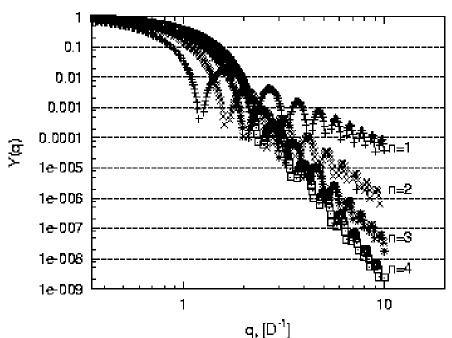
Figure 4: Functions $Y(q)$ correspondent to $P(r)$ shown in Fig.3

A negative, inevitable consequence of high $\nu$ order implementation is the decrease in light transmission $\gamma$ and so a weak light signal. Thus a certain trade-off exists between good filtration of image motion and a high signal level that is necessary for image centroiding.

5 Reference frames with a virtual symmetry

Consider a vector quantity $\@vec{W}$ with two components

$$\begin{array}[]{l}W_{x}=N^{-1}\sum_{i=1}^{N}a_{i}(\bar{x}_{0}-\bar{x}_{i})=\bar{x}_{0}-N^{-1}\sum_{i=1}^{N}a_{i}\bar{x}_{i}\\ W_{y}=N^{-1}\sum_{i=1}^{N}a_{i}(\bar{y}_{0}-\bar{y}_{i})=\bar{y}_{0}-N^{-1}\sum_{i=1}^{N}a_{i}\bar{y}_{i}\end{array}$$ (19)

formed by a linear combination of measured (instant image motion included) differences of Cartesian coordinates of the target $\bar{x}_{0}$, $\bar{y}_{0}$ and $i$-th reference star $\bar{x}_{i}$, $\bar{y}_{i}$, $i=1,2..N$ scaled at the phase screen height $h$; $a_{i}$ are some weights that satisfy a normalizing condition

$$\sum_{i=1}^{N}a_{i}=N.$$ (20)

Introduction of the quantity (19) instead of normally non-weighted differential positions reduces the problem of image motion suppression to the qualification of conditions on $a_{i}$ which minimize the variance of $\@vec{W}$. A peculiarity of this study is the permission to use any, even negative, weights $a_{i}$. The vector $\@vec{W}$ that defines the differential position of the target object relative to the weighted center of reference group $N^{-1}\sum a_{i}\bar{x}_{i}$, $N^{-1}\sum a_{i}\bar{y}_{i}$ is the only quantity which can be measured with high precision. Therefore, the possibility to extract positional information from $\@vec{W}$ is not obvious and will be discussed in Section 7.

Besides atmospheric noise, the total error of observations depends also on the image-centroiding error component $\sigma_{ph}$ in $\@vec{W}$ caused by a Poisson photon noise in star images. Assuming that $D_{i}$ is the variance of the $i$-th reference star centroid position caused by photon noise, we find from Eq.(19)

$$\sigma^{2}_{ph}=N^{-2}\sum_{i=1}^{N}a^{2}_{i}D_{i}$$ (21)

since a contribution from the usually bright target object is small. For Gaussian shaped images with r.m.s. width $\sigma_{0}=\mbox{FWHM}/2.36$ and $n_{i}$ detected photons, an expression (Irwin 1985)

$$D_{i}=\sigma_{0}^{2}/n_{i}$$ (22)

is valid for sufficiently bright images with a light signal exceeding photon noise.

5.1 Functions $Q(q)$ of high $k$-orders

Expressions for differential image motion effects derived in Sections 2 – 3 in application to the double star observations can be easily extended to the case of a measured value $\@vec{W}$. Image motion for the quantity (19) is now expressed through the weighted differences of the function $\zeta$ values in points B₀ and B_i: $\Delta\zeta=N^{-1}\sum_{i}a_{i}[\zeta(B_{0})-\zeta(B_{i})]$. The difference operator (7) corresponding to $\Delta\zeta$ and the geometry shown in Fig.1 is then

$$\tilde{Q}({\bf r,s})=N^{-1}\sum_{i}a_{i}[\delta({\bf r})-\delta({\bf r+s}_{i})]$$ (23)

A Fourier transform of this expression with a subsequent integral averaging (10) yields a function

$$Q(q)=N^{-2}\sum_{i,j=1}^{N}a_{i}a_{j}[1-2J_{0}(2\pi qs_{i})+J_{0}(2\pi qs_{ij})]$$ (24)

corresponding to a new definition of the measured quantity. Analysis of Eq.(24) permits us to formulate the conditions necessary to increase the $Q(q)$ function order. For this purpose we expand the Bessel functions in (24) into power series of $q$, deriving the approximation at low frequencies:

$$\begin{array}[]{ll}Q(q)&=\frac{1}{N^{2}}\sum_{m=1}^{\infty}\frac{(-1)^{m+1}}{(m!)^{2}}(\pi q)^{2m}\sum_{i,j=1}^{N}a_{i}a_{j}\\ &\\ &\times(s_{i}^{2m}+s_{j}^{2m}-s_{ij}^{2m})\end{array}$$ (25)

The order $k$ of the $Q(q)$ function is determined by the first non-zero term in the expansion; normally, $k=2$ if no special efforts are made.

With $s_{i}$, $s_{ij}$ fixed, one may always choose a set of coefficients $a_{i}$ turning to zero the first or few first sum values $\sum_{i,j=1}^{N}a_{i}a_{j}(s_{i}^{2m}+s_{j}^{2m}-s_{ij}^{2m})$ which are coefficients at $q^{2m}$. With a sufficiently large number of reference stars, all the first $q^{2},q^{4}\ldots q^{k-2}$ expansion terms in (25) could be eliminated by applying conditions

$$\begin{array}[]{l}\sum\sum a_{i}a_{j}(s_{i}^{2}+s_{j}^{2}-s_{ij}^{2})=0,\\ \sum\sum a_{i}a_{j}(s_{i}^{4}+s_{j}^{4}-s_{ij}^{4})=0,\\ \ldots\\ \sum\sum a_{i}a_{j}(s_{i}^{k-2}+s_{j}^{k-2}-s_{ij}^{k-2})=0\end{array}$$ (26)

where $k$ is some even integer. Under conditions (26), the power of the first non-zero term in the expansion (25) can be increased from normal $k=2$ to some higher $k\geq 4$. Eq.-s(26) is a system with unknowns $a_{i}$; it includes only a single first line at $k=4$, the two first lines at $k=6$, and so on. The system (26) can be converted to a simpler form. Thus, passing to Cartesian coordinates $x_{i}-x_{0}=s_{i}\cos\psi_{i}$, $y_{i}-y_{0}=s_{i}\sin\psi_{i}$ and taking into consideration Eq.(20) one finds that each sum of sums in Eq.-s(26) takes the form of products of one-dimensional sums. For instance, the first equation leading to $k=4$ transformes to

$$\sum\sum a_{i}a_{j}(s_{i}^{2}+s_{j}^{2}-s_{ij}^{2})=2(M_{x}^{2}+M_{y}^{2})=0$$ (27)

where $M_{x}=\sum a_{i}(x_{i}-x_{0})$ and $M_{y}=\sum a_{i}(y_{i}-y_{0})$ are the first coordinate moments. The next equation, for $k=6$, $\sum\sum a_{i}a_{j}(s_{i}^{4}+s_{j}^{4}-s_{ij}^{4})=2[\sum a_{i}(x_{i}-x_{0})^{2}+\sum a_{i}(y_{i}-y_{0})^{2}]^{2}+4[\sum a_{i}(x_{i}-x_{0})^{2}]^{2}+4[\sum a_{i}(y_{i}-y_{0})^{2}]^{2}+8[\sum a_{i}(x_{i}-x_{0})(y_{i}-y_{0})]^{2}=0$ contains quadratic cross-moments. Direct computations show that the order of cross-moments is incremented by 1 when passing to each next $k$ order. The quadratic form of the equations suggests that all weighted cross moments of reference star coordinates are zero. An equivalent form of system (26) is therefore

$$\begin{array}[]{l}\sum a_{i}=N,\\ \sum a_{i}(x_{i}-x_{0})=\sum a_{i}(y_{i}-y_{0})=0,\\ \sum a_{i}(x_{i}-x_{0})^{2}=\sum a_{i}(x_{i}-x_{0})(y_{i}-y_{0})=\\ =\sum a_{i}(y_{i}-y_{0})^{2}=0,\\ \ldots\\ \sum a_{i}(x_{i}-x_{0})^{\frac{k}{2}-1}=\sum a_{i}(x_{i}-x_{0})^{\frac{k}{2}-2}(y_{i}-y_{0})=\\ \ldots=\\ \sum a_{i}(x_{i}-x_{0})(y_{i}-y_{0})^{\frac{k}{2}-2}=\sum a_{i}(y_{i}-y_{0})^{\frac{k}{2}-1}=0\end{array}$$ (28)

which reveals the modal structure of the filter $Q(q)$. At $k=2$, when none of conditions (26) are fulfilled, the system is limited by a single first line normalizing equation; at $k=4$ it includes the first two lines (three equations), and so on; the total number of equations is $k(k+2)/8$. In a compact form, the system (28) with unknowns $a_{i}$ is written as

$$\begin{array}[]{lr}\sum a_{i}=N,&\\ \sum a_{i}(x_{i}-x_{0})^{\alpha}(y_{i}-y_{0})^{\beta}=0,&\;\alpha+\beta=1\ldots\frac{k}{2}-1,\end{array}$$ (29)

where $\alpha$ and $\beta$ are positive integers. The use of weights $a_{i}$ satisfying Eq.-s(29) results in elimination of $k/2-1$ first terms in the expansion (25) which becomes

$$\begin{array}[]{ll}Q(q)&=\frac{1}{N^{2}}\sum_{m=k/2}^{\infty}\frac{(-1)^{m+1}}{(m!)^{2}}q^{2m}\sum_{i,j=1}^{N}a_{i}a_{j}\\ &\\ &\times(s_{i}^{2m}+s_{j}^{2m}-s_{ij}^{2m})\end{array}$$ (30)

It should be noted that in the case of $k\geq 6$ when quadratic moments of $x$ and $y$ are involved in Eq.-s(29), the solution must incorporate negative $a_{i}$ values, which is rather unusual for a common technique of astrometric reductions.

Application of various sets of $a_{i}$ changes the geometric properties of a reference group. Thus, implementation of $a_{i}$ of the $k=4$ order for which condition $\sum a_{i}(x_{i}-x_{0})=\sum a_{i}(y_{i}-y_{0})=0$ is fulfilled transforms an arbitrary reference group into its virtual equivalent with an ideal symmetric structure centered at the point $x_{0}$, $y_{0}$. With respect to the image motion statistics, and the filter $Q(q)$ asymptotic behaviour in particular, both groups become indistinguishable providing they are of equal effective size. A further increase of $k$ results in enhanced improvement of reference group filtering properties which can reveal a power dependency stronger than $Q(q)\sim q^{4}$, a case impossible with a simple geometric symmetry.

Implementation of high $k$ orders is limited by the number $N$ of reference stars available. The minimum $N$ value required to achieve some $k$ order and to find solutions $a_{i}$ of the system (29) is

$$N_{min}=\left\{\begin{array}[]{lr}k(k+2)/8,&\mbox{for 2-D distribution of stars}\\ k/2,&\mbox{for 1-D, in-line distribution}\end{array}\right.$$ (31)

Here we admitted that $N_{min}$, generally, depends on the type of star distribution in the field. Though exactly linear configurations do not exist, they serve well for illustrative purposes.

At $N>N_{min}$, a redundancy of the system (29) allows us to set a useful (even in the case of $k=2$) condition

$$\sum a^{2}_{i}D_{i}=\mbox{min}$$ (32)

which reduces the centroiding error (21). A consistent solution of (29) and (32) is found with a standard Lagrangian method of undetermined coefficients. Such a solution is optimal with respect to both atmospheric and photon centroiding errors.

5.2 Tutorial linear configurations

Some tutorial examples of linear (along the $x$-axis) configurations are given in Table 2 which contains the conditional name of configurations, $x$-coordinates of stars given with reference to the target and expressed in seconds of arc, $a_{i}$ values, $\overline{a^{2}}=N^{-1}\sum a_{i}^{2}$ and the principal $q^{k}$ term of the $Q(q)$ function expansion. $x_{i}$ are scaled to equalize the effective angular size of each group to $\rho=1^{\prime}$. For a turbulent layer at $h=20$ km, this angle corresponds to an effective linear size $S=\rho h=5.82$ m. The last quantity is convenient to define as

$$S=\left|N^{-2}\sum_{ij}^{N}a_{i}a_{j}(s_{i}^{k}+s_{j}^{k}-s^{k}_{ij})\right|^{1/k}$$ (33)

which relates $S$ to the magnitude of the first non-zero term in the expansion (25). A convenience of this definition is that series expansion (30) (its leading term) is now simplified to

$$Q(q)=(\pi qS)^{k}/[(k/2)!]^{2}$$ (34)

Note that effective sizes $S$ and $\rho$ depend very weakly on the peculiarities of the star distribution in the frame and approximately are equal or slightly exceed its radius (the largest separation target-reference star).

Table 2: Linear configurations of effective angular size $\rho=1^{\prime}$ and $k$-order virtual symmetry

Name	$N$	$k$	$x_{i}$	$a_{i}$	$\overline{a^{2}}$	$Q(q)$
a	1	2	42′′	1	1	$q^{2}$
b	2	4	-38, 38	1, 1	1	$q^{4}$
c	2	4	27, 54	4, -2	10	$q^{4}$
d	3	6	-29, 29, 58	1, 3, -1	3.67	$q^{6}$
e	3	4	-32, 32, 64	12/7,6/7,3/7	9	$q^{4}$
f	4	4	-31$\sqrt{2}$, -31,
			31, 31$\sqrt{2}$	1, 1, 1, 1	1	$q^{4}$
g	4	8	-30$\sqrt{2}$, -30,
			30, 30$\sqrt{2}$	-2, 4, 4, -2	10	$q^{8}$
h	6	12	-56,-37.4,-18.7,	0.3,-1.8,4.5,
			18.7,37.4,56	4.5,-1.8,0.3	7.9	$q^{12}$

Table 2 shows that even strongly asymmetric star groups ”c” and ”d” are subject to high order symmetrization. This is achieved, however, at the expense of applying large $a_{i}$ owing to which the $\overline{a^{2}}$ value is greater than that for symmetric groups (compare cases ”b” and ”c”). Thus, application of high order symmetry for asymmetric star groups reduces atmospheric noise but causes a rise of the centroiding error (21). The same effect is observed even for symmetric distributions ”g” and ”h” when very high $k$ is used.

Figure 5: Functions $Q(q)$ for stellar groups ”a, c, d, g” (Table 2) with $k=2$, 4, 6 and 8 symmetry order; $D/S=17.2$

The $Q(q)$ plots shown in Fig.5 for a few configurations of Table 2 emphasize a difference in the function form at low frequencies which for both symmetric and non-symmetric star distributions is determined only by the index $k$. Asymmetry of star groups ”c” and ”d” leads to the increase of amplitude $Q_{\infty}$ of $Q(q)$ at high frequencies $q\geq 1/S$, which, due to relation $\overline{a^{2}}/N=Q_{\infty}-1$ following from Eq(24), is indicative of the $\sigma^{2}_{ph}$ increase.

An example of 2-D stellar group symmetrization is given in Table 3 for a sample of $N=14$ stars of the open cluster NGC 2420 observed with the 5-m Palomar telescope (Pravdo & Shaklan 1996). The table contains star coordinates $x_{i}$, $y_{i}$ with reference to the target star, weights $a_{i}$ and $\overline{a^{2}}=\sum a_{i}^{2}/N$ for various orders up to $k=8$. Weights $a_{i}$ were computed using conditions (32) with $D_{i}=\mbox{const}$. The extremally small angle $\rho=3.7^{\prime\prime}$ found at $k=2$ is by no means due to a special selection of reference stars (no selection was applied) and reflects the effect of field averaging making the first moments $M_{x}$ and $M_{y}$ small for large $N$. In the limit of $N\to\infty$, discussed in Section 6, any $k=2$ order group is moved up to the 4-order. Note also that the value of $\overline{a^{2}}$ is rapidly increasing with $k$, so does the variance (21).

Table 3: Weights $a_{i}$ symmetrizing a stellar group (Pravdo & Shaklan 1996) to $k=2\ldots 8$ orders

			$k$
$x_{i}$	$y_{i}$	2	4	6	8
46.0′′	19.4′′	1.0	0.914	-1.355	-0.023
33.5	17.1	1.0	0.908	0.340	-1.120
19.1	18.7	1.0	0.845	0.739	0.680
9.5	16.1	1.0	0.851	1.792	0.308
-3.2	5.7	1.0	0.951	3.414	3.300
17.1	3.4	1.0	1.039	3.201	4.300
8.8	-11.4	1.0	1.209	1.787	7.102
14.6	-15.7	1.0	1.282	0.624	-0.265
19.2	-16.1	1.0	1.300	0.465	-2.793
-24.1	1.1	1.0	0.950	2.981	2.157
-32.5	-4.7	1.0	1.002	1.940	2.362
-41.3	-8.6	1.0	1.028	0.572	-1.593
-36.3	-16.4	1.0	1.144	-1.407	-0.138
-45.5	24.9	1.0	0.578	-1.092	-0.278
$\overline{a^{2}}$		1.0	1.03	3.40	7.32
$\rho$		3.7′′	45.7′′	35.2′′	42.2′′

5.3 Expressions for the variance of image motion

Analytic expressions for $\Delta^{2}$ in a limiting case of very long exposures and narrow fields $T\gg D/V\gg S/V$ can be derived from Eq.(12) where $Y(q)$ and $Q(q)$ are given by Eq.-s(18) and (24):

$$\begin{array}[]{ll}\Delta^{2}&=\frac{\lambda^{2}c_{\phi}2^{\nu-1}\left(\frac{\nu-1}{2}!\right)^{2}}{N^{2}VT}\int\limits_{0}^{\infty}\frac{J_{(\nu-1)/2}^{2}(\pi Dq)}{(\pi Dq)^{\nu-1}}\sum\sum a_{i}a_{j}[1-\\ &-2J_{0}(2\pi qs_{i})+J_{0}(2\pi qs_{ij})]q^{-1-p}\,dq\end{array}$$ (35)

An approach to integration depends on the ratio between the $k$ and $\nu$ values. When $k>\nu+p$, the integral converges at $q=0$ so approximation (14) for $Y(q)$ is valid. Integrating by parts and taking advantage of the condition (26) results in

$$\begin{array}[]{l}\Delta^{2}=\frac{\lambda^{2}c_{\phi}2^{\nu}\left(\frac{\nu-1}{2}!\right)^{2}\hat{S}^{\nu+p}}{4{\pi}^{1-p}VTD^{\nu}{\Gamma}^{2}(\frac{p+\nu+2}{2})}\left\{\begin{array}[]{ll}\Gamma(\frac{p+1}{2})\Gamma(\frac{1-p}{2}),&\nu\mbox{- odd}\\ \Gamma(\frac{p}{2})\Gamma(\frac{2-p}{2}),&\nu\mbox{- even}\\ \end{array}\right.\\ k>\nu+p\\ \end{array}$$ (36)

Here $\hat{S}={|N^{-2}\sum\sum a_{i}a_{j}[2{s_{i}}^{p+\nu}-{s_{ij}}^{p+\nu}]|}^{1/(p+\nu)}$ is a modified field size defined similarly to (33) but with fractional powers. Since $s_{i}=s\rho_{i}/\rho$, from (36) we find a power dependency $\Delta^{2}\sim S^{\nu+p}/D^{\nu}$ which is in agreement with Eq.(15) and Table 1 testifying that an increase of $k$ over $\nu+p$ does not affect the power laws. Another interesting point is the dependency of $\Delta$ on $k$ which, however, is not clear from (26) since it contains the $\hat{S}$ term related to $k$ via weights $a_{i}$. A rough expression for $\Delta$ with no $\hat{S}$ term can be obtained based on the next Sections results for non-discrete star fields. Using approximation (49) for $Q(q)$ and recomputing the integral (12) with $Y(q)$ given by (14), yields

$$\begin{array}[]{ll}\Delta^{2}=\frac{\lambda^{2}c_{\phi}2^{\nu-1}{(k/4)}^{k-\nu-p}{(\frac{\nu-1}{2}!)}^{2}{S}^{\nu+p}}{VT{[(k/2)!]}^{2}(k-\nu-p)D^{\nu}}&,k>\nu+1\\ \end{array}$$ (37)

which is a decreasing function of $k$ at $\nu$ fixed. The use of high $k$ orders, thus, always reduces atmospheric noise.

At $k<\nu+p$, the integral (35) is calculated with approximation (34) for $Q(q)$. Direct integration yields

$$\begin{array}[]{l}\Delta^{2}=\frac{\lambda^{2}c_{\phi}2^{\nu-2}{\pi}^{p}{(\frac{\nu-1}{2}!)}^{2}\Gamma(\frac{k-p}{2})\Gamma(\frac{\nu+p-k}{2})S^{k}}{VT{[(k/2)!]}^{2}\sqrt{\pi}D^{k-p}\Gamma(\nu+\frac{p-k}{2})\Gamma(\frac{\nu+p+1-k}{2})}\\ k<\nu+p\\ \end{array}$$ (38)

and is also consistent with Table 1. It should be stressed that, unlike the previous case of $k>\nu+p$, an increase of $\nu$ over $k$ gives rise to $\Delta^{2}$. The deterioration of the results is related to the expansion of the filter $Y(q)$ nucleus width, clearly seen in Fig.4.

6 Virtual symmetry for dense reference frames

Approximate characteristics of reference groups with several stars are easily found in a limit of infinite $N$ when the star distribution becomes continuous. All estimates are found especially easily since discrete summations are substituted by integrals, and individual features of star distribution in the field become unimportant.

6.1 Approximate expressions for $a_{i}$ and $\sigma_{ph}$

We assume equal brightness of stars. Assuming also that reference stars are evenly distributed around the target in a circle of radius $R$ with a spatial density $N/(\pi R^{2})$, we introduce, instead of weights $a_{i}$, a weighting function $a(r)$ with a radial symmetry which satisfies the normalizing condition $\frac{N}{\pi R^{2}}\int_{0}^{R}a(r)\,dx\,dy=N$ equivalent to (20). For a $k$-order function $Q(q)$, an integral analogue of the system of equations (29) with unknown function $a(r)$ is

$$\begin{array}[]{ll}\int_{0}^{R}a(r)r\,dr=R^{2}/2,&k=4\\ \int_{0}^{R}a(r)r^{\alpha}\,dr=0,&\alpha=1,3\ldots\frac{k-2}{2},k=8,12\ldots\\ \end{array}$$ (39)

The above system is valid for $k$ multiples of 4 only, since for any symmetric distributions Eq.-s (29) with coordinate cross-moments of odd powers are satisfied automatically; for this reason orders $k=2,6,10\ldots$ do not exist, they are moved up into the next higher order. Considering only a polynomial class of solutions for $a(r)$ of the form $a(r)=b_{0}+b_{2}r^{2}+\ldots+b_{\beta}r^{\beta}$, where $\beta=k/2-2$, and performing integration (39), we come to a linear system of $\beta/2+1$ equations with respect to unknowns $b_{2j}$:

$$\sum_{j=0}^{\beta/2}\frac{b_{2j}R^{2j}}{2(i+j+1)}=\left\{\begin{array}[]{l}R^{2},\;i=0\\ 0,\;i=1,2\ldots\beta/2\end{array}\right.$$ (40)

The solution found by computer simulation is

$$\begin{array}[]{l}a(r)=\frac{k}{4}\sum_{i=1}^{k/4}(-1)^{i+1}\frac{(k/4-i+1)!}{(k/4-i)!i!(i-1)!}\left(\frac{r}{R}\right)^{2i-2},\\ k=4,8\ldots;\;\;r\leq R\end{array}$$ (41)

Figure 6: Weighting functions (42) for circular star distributions at $k=4$, 8, 12; the asymptotic form (43) of $a(r)$ at $k=12$

For a few first $k$, the weighting functions

$$a(r)=\left\{\begin{array}[]{ll}1,&k=4\\ 2(2-3r^{2}/R^{2}),&k=8\\ 3(3-12r^{2}/R^{2}+10r^{4}/R^{4}),&k=12\end{array}\right.$$ (42)

are shown in Fig.6. Except for the case of $k=4$ discussed by Lindegren (1980) and when $a(r)=$const, the plots of $a(r)$ incorporate some oscillating circular zones coming from the field outer borders. The number of these zones and the function’s peak increases with $k$ while the amplitude of oscillations decreases. These features are easily explained since Eq.(41) at $k\to\infty$ is reduced to $a(r)=(k/4)^{2}\sum_{i=0}^{k/4-1}(-1)^{i}[kr/(4R)]^{2i}/[i!(i+1)!]$ which is a truncated power expansion of the Airy-type oscillating function

$$a(r)=\left(\frac{k}{4}\right)^{2}\frac{2J_{1}(\frac{kr}{2R})}{kr/(2R)}$$ (43)

For comparison, the asymptotic and exact forms of $a(r)$ for $k=12$ are shown in Fig.6.

Above we assumed equal brightness of field stars. Let us find expressions for a weighting function $a(r,D_{i})$ that approximates weights $a_{i}$ for descrete very dense distributions while accounting for magnitude-dependent centroiding variances $D_{i}$ (22). In this case the condition (32) leads to the inverse proportion $a_{i}\sim 1/D_{i}$, which follows also from a least-squares principle. Assuming that spatial and brightness distribution of stars in the field are uncorrelated and using $a(r)$ as approximation for $a_{i}$ at $D_{i}=$const, we obtain

$$a(r,D_{i})\simeq a(r)\frac{D_{1}}{D_{i}}$$ (44)

where $D_{1}=N/\sum_{i=1}^{N}D_{i}^{-1}$ is the mean (effective) variance of one reference star. The total centroiding variance of all reference field than is $D_{\rm{eff}}=D_{1}/N=1/\sum D_{i}^{-1}$ . Taking Eq.(22) into consideration, we find

$$D_{\rm{eff}}=\sigma_{0}^{2}/\sum n_{i}.$$ (45)

Incorporating fainter stars, a value of $D_{\rm{eff}}$ always decreases (improves) but rapidly approaches some limit.

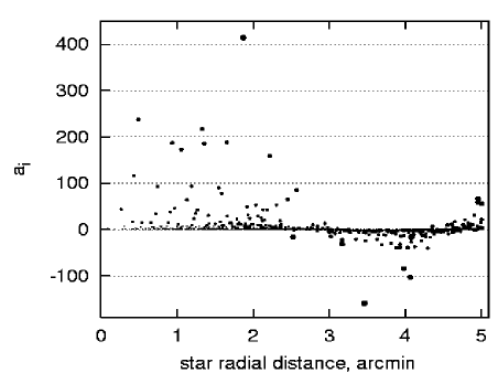
Figure 7: An example of $a_{i}$ coefficients symmetrizing a random $5^{\prime}$ field with 3170 stars to the $k=12$ order; dot sizes are proportional to the star brightness (12 to 23 mag)

The above considerations are illustrated by a numerical simulation of a random 5^′ field (radius) with 3170 stars. The magnitude and sky star distribution corresponds to the Galaxy model (Bahcall & Soneira 1980) and galactic coordinates $b=20^{0}$, $l=0^{0}$. The field with stars to V=23 mag was symmetrized to the $k=12$ order; a distribution of computed $a_{i}$ values versus distance from the field center is shown in Fig.7. In this example an accumulated value of $D_{\rm{eff}}$ is equivalent to that produced by 120.3 stars of 15 mag; an effective mean centroiding variance of one reference star $D_{1}$ corresponds to the star of V=18.5 mag. A large scatter of computed $a_{i}$ values seen in Fig.7 is natural since $a_{i}\simeq 1/D_{i}$; this relation is exact at $k=2$ and becomes rough at large $k$. Usually, $|a_{i}|\gg 1$ for bright and $|a_{i}|\ll 1$ for faint images. Sampled values of $a_{i}D_{i}/D_{1}$, on the contrary, show small scatter and a strong concentration around the $a(r)$ function plot (Fig.8). Approximate values of $a_{i}$ thus can be found from Eq.(44) for any $k$ star.

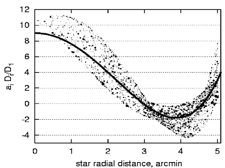
Figure 8: $a_{i}D_{i}/D_{1}$ values for random data shown in Fig.7; solid line - approximation by the function $a(r)$ plotted for $k=12$

An increase of the $a(r)$ amplitude in the field center for high $k$ leads to an increase of the total centroiding error $\sigma^{2}_{ph}$. This effect is easily estimated since, with above the assumptions, the magnitude-related $D_{i}$ and coordinate-related $a_{i}^{2}$ terms in Eq.(21) are statistically independent. Therefore Eq.(21) transforms to $\sigma^{2}_{ph}=D_{\rm{eff}}\overline{a^{2}}$ where $\overline{a^{2}}=(\pi R^{2})^{-1}\int\int a^{2}(r)\,dx\,dy$ is an averaged value of $a(r)$. Direct integration of Eq.(42) yields $\overline{a^{2}}=(k/4)^{2}$ whence

$$\sigma^{2}_{ph}=D_{\rm{eff}}(k/4)^{2}$$ (46)

The last equation can be given in terms of star image parameters. Taking into consideration Eq.(22) and allowing for light transmission $\gamma$ of the apodized objective Eq.-s(18), we obtain

$$\sigma_{ph}=\frac{\mbox{FWHM}}{2.36\sqrt{\sum n_{i}}}(k/4)\sqrt{\frac{\nu-1}{2}}$$ (47)

The photon noise thus depends on FWHM, the total light of reference stars $\sum n_{i}$, $k$ and $\nu$. The use of very faint stars as a reference clearly does not lead to improvement in $\sigma_{ph}$ because their contribution to $\sum n_{i}$ is negligible; the use of very high $k$ orders degrades $\sigma_{ph}$.

6.2 Expressions for $Q(q)$ and $S$

The asymptotic form of the function $Q(q)$ for stars of equal brightness is found from a limiting ($N\to\infty$ ) form of the function (23) which is $\tilde{Q}({\bf r})=\delta({\bf r})-P({\bf r})a({\bf r})/(\pi R^{2})$. From this it follows that $Q(q)={\mathcal{F}}^{2}\{\tilde{Q}\}=[1-2R^{-2}\int_{0}^{R}a(r)J_{0}(2\pi rq)r\,dr]^{2}$ , and a direct integration with $a(r)$ given by Eq.(42) yields

$$Q(q)=\left\{\begin{array}[]{ll}[1-2J_{1}(2\pi Rq)/(2\pi Rq)]^{2},&k=4\\ \left[1+\frac{4J_{1}(2\pi Rq)}{(2\pi Rq)}-\frac{24J_{2}(2\pi Rq)}{(2\pi Rq)^{2}}\right]^{2},&k=8\\ &\\ \left[1-\frac{6J_{1}(2\pi Rq)}{(2\pi Rq)}+\frac{96J_{2}(2\pi Rq)}{(2\pi Rq)^{2}}-\right.&\\ \left.-\frac{480J_{3}(2\pi Rq)}{(2\pi Rq)^{3}}\right]^{2},&k=12\\ \ldots&\\ \left\{\begin{array}[]{ll}0,&q<k/(4\pi R)\\ 1,&q>k/(4\pi R)\end{array}\right.&k\to\infty\\ \end{array}\right.$$ (48)

An expression for $k\to\infty$ derived with a Hankel transform of Eq.(43) shows that an asymptotic form of $Q(q)$ is an opaque circle with radius proportional to $k$. Expansion of Eq.-s(48) into power series of $q$ yields an expression

$$Q(q)=\left\{\begin{array}[]{ll}\frac{(\pi Rq)^{k}}{[(k/2)!]^{2}},&q<k/(4\pi R)\\ 1,&q>k/(4\pi R)\end{array}\right.$$ (49)

valid for $k=4,8\ldots$. Comparing this expression with a definition (34) for effective size $S$, we come to a very simple relation

$$S=\begin{array}[]{lrr}R,&k/2&\mbox{even}\\ \end{array}$$ (50)

Figure 9: Effective field size $S_{\rm{rnd}}$ versus radius $R$ of random samples at high star density; $k$ is the reference group symmetry order; lines are data fits (51)

To test the validity of Eq.(50), we performed numerical simulations that assumed the Galaxy model by Bahcall & Soneira (1980). Random star samples taken in the near-equatorial zone ($b=20{\degr}$, $l=0{\degr}$) to V=23 mag were symmetrized, with condition (32), to $k=2,4..12$ order and estimates $S_{\rm{rnd}}$ of $S$ for each random sample were computed using Eq.(33). Random sizes $S_{\rm{rnd}}$ presented in Fig.9 are fitted with the function

$$S_{\rm{exp}}=\chi R^{\mu}$$ (51)

that gives the expectation of effective field size for a random star sample taken in a circle of a radius $R$; both $S_{\rm{exp}}$ and $R$ are given in arcminutes. The model (51) is consistent with (50) and extends this dependency to odd $k/2$. The quantities $\chi$ and $\mu$ valid for both high and low star density are given in Table 4. At polar regions, the values of these parameters are higher, thus slightly larger $S$ and $\Delta$ are expected at equal $R$.

Table 4: Coefficients of Eq.(51) for different star density

	near-equatorial zone		Galactic pole
$k$	$\chi$	$\mu$	$\chi$	$\mu$
2	0.275	0.414	0.848	0.537
6	0.712	0.817	1.000	0.830
10	0.857	0.893	0.997	0.922
$\chi=\mu=1$ for $k=4,8,12$ ($k/2$ even)

For $k/2$ odd the value of $S$ is a function of odd-order coordinate cross-moments averaged over the field. Result of averaging depends largely on the contribution from a few bright stars with large $a_{i}$ and so is not returned to zero as it is expected for star fields with constant star brightness. Not performing a detailed study, we assumed that in the spectral domain this effect is described by the empiric model

$$\begin{array}[]{ll}Q(q)=&Q_{k+2}(q)+(S/R)^{k}[J^{2}_{k/2}(2\pi Rq)+\\ &+2\sum\limits_{m=k/2+1}^{\infty}J^{2}_{m}(2\pi Rq)],\;\>k/2\;\>{\mbox{odd}}\end{array}$$ (52)

with correct asymptotic properties. Here $Q_{k+2}(q)$ is a $k+2$ order function (48); $S$ is given either by Eq.(51) to produce the mathematical expectation of the filter or is a sampled field size leading to a ”sampled” filter. The second component in the expression is caused by incomplete averaging of odd-order coordinate moments and decreases with $R$ since $(S/R)<1$. For fields with stars of equal brightness, this component vanishes yielding $Q(q)=Q_{k+2}(q)$ and thus increasing the field symmetry order by +2. It is easy to find that Eq.(52) at short $q$ follows approximation (34), critically important for computation of $\Delta$. Direct calculations of $\Delta$ for random star fields in Sect.9 had proved the validity of the model (52).

Finally let us derive laws for $\Delta$ as a function of reference star number $N$ in the field, and its radius. As follows from Eq.(31), the field symmetry order not can exceed $k_{\rm{max}}=\sqrt{8N+1}-1$. Then, with some optional $k\leq k_{\rm{max}}$ and optimal apodization parameter $\nu=k$ or $\nu=k+1$ (Table 1), we find that for a turbulent layer at a height $h$

$$\Delta^{2}\sim\chi^{k}\left[{\frac{hR}{3400D}}\right]^{k}R^{k(\mu-1)}D^{2/3}$$ (53)

where $R$ is in arcminutes, $D$ and $h$ in meters. Consider that at high star density, a $R=1^{\prime}$ field is expected to contain about 100 stars to V=23 mag; using all of them as reference makes $k$ orders to $k_{\rm{max}}\approx 25$–30 quite feasible. A gain in $\Delta$ for narrow $hR<3400D$ fields is therefore huge.

7 Plate reduction

An approach to plate reduction based on the current technique should take into account the fact that effective filtration of atmospheric noise occurs only in a two-component vector $\@vec{W}$. As opposed to the common technique based on plate constant determination that provides a global fitting of measured to model data at any point on the plate, the present technique gives a local solution valid directly at the point $x_{0}$, $y_{0}$. When multiple targets are considered, each one should be processed with its own set of weights $a_{i}$ centered on the particular target. Below we explain in detail the feasibility of recovering positional information from the quantity $\@vec{W}$, taking into account the two possible goals of observations:

– determination of the target object position with reference to field stars, using their precise positions (a classic problem of astrometry), and

– determination of the target proper motion with reference to field stars (positions unknown) from observations made in the two epochs.

7.1 Compensation of low-order reduction model terms in $\@vec{W}$

Consider polynomial expansion

$$\begin{array}[]{ll}\bar{x}_{i}&=x_{i}+A_{0}+A_{1}^{1,0}(x_{i}-x_{0})+A_{1}^{0,1}(y_{i}-y_{0})\\ &+A_{2}^{2,0}(x_{i}-x_{0})^{2}+A_{2}^{1,1}(x_{i}-x_{0})(y_{i}-y_{0})\\ &+A_{2}^{0,2}(y_{i}-y_{0})^{2}+\ldots=x_{i}+A_{0}\\ &+\sum\limits_{m=1}^{k/2-1}\sum\limits_{\begin{array}[]{c}{}^{\alpha,\beta=0,}_{\alpha+\beta=m}\end{array}}^{m}A_{m}^{\alpha,\beta}(x_{i}-x_{0})^{\alpha}(y_{i}-y_{0})^{\beta}\\ &+{\mathcal{R}}_{k/2}(x_{i}-x_{0},y_{i}-y_{0})\end{array}$$ (54)

of star measured coordinates $\bar{x}_{i}$, $\bar{y}_{i}$ over coordinate cross-moments $m=1,2\ldots k/2-1$ of actual coordinates $x_{i}$, $y_{i}$ not distorted by the atmosphere; the equation for $y$ has a similar structure and all coordinates are considered to be scaled to the turbulent layer height $h$. Expansion (54) is essentially a reduction model used for fitting measured to standard coordinates. The first few modes of the expansion with amplitudes $A_{m}^{\alpha,\beta}$ represent common geometric terms: zero-point (mode $m=0$) and scale ($m=1$), also, they can be associated with the influence of the classic optical aberrations: tilt ($m=0$), defocus and astigmatism ($m=1$), etc.

Each expansion term $A_{m}^{\alpha,\beta}$ may include also a stochastic component of image motion which, due to a similar structure of Eq.-s (54) and (29) is associated with a corresponding modal term of the $Q(q)$ function. The model is truncated by some $k/2-1$ order; the sum of high $m\geq k/2$ modes is denoted as ${\mathcal{R}}_{k/2}$.

An expression for the $W_{x}$ quantity is found by subtracting from (54) an identity $\bar{x}_{0}=A_{0}+x_{0}$ valid at the point $x_{i}=x_{0}$, $y_{i}=y_{0}$ and performing a summation with $a_{i}$:

$$\begin{array}[]{ll}W_{x}&=\frac{1}{N}\sum a_{i}(\bar{x}_{0}-\bar{x}_{i})\\ &=-\frac{1}{N}\sum a_{i}{\mathcal{R}}_{k/2}(x_{i}-x_{0},y_{i}-y_{0})\end{array}$$ (55)

Here all $A_{1}$, $A_{2}\ldots A_{k/2-1}$ low-order components vanish due to conditions (29). The use of weights $a_{i}$ based on the true differential position of stars $x_{0}-x_{i}$, $y_{0}-y_{i}$ therefore allows us to form a linear combination (55) of measured coordinates which is insensitive to low-order terms of expansion (54), irrespective of whether they are constant or stochastic ones. It is very important that $W_{x}$ does not depend on any changes of aberrations and temporal variations of image motion of low orders. The mathematical expectation of $W_{x}$ thus is zero and its variance depends on high $k/2$, $k/2+1\ldots$ modes uncompensated in the summation.

7.2 Determination of target position

Formulation of this particular problem implies that the precise position $x_{obj}$, $y_{obj}$ of the target object is unknown and $x_{0}$, $y_{0}$ is a preliminary object’s position used for computation of weights $a_{i}$. The true target position $x_{obj}=x_{0}+\delta x$ ($\delta x$ is a correction to $x_{0}$) is related, as it follows from (54), to a measured position $\bar{x}_{obj}=x_{0}+\delta x+A_{0}+A_{1}^{1,0}\delta x+A_{1}^{0,1}\delta y+A_{2}^{2,0}\delta x^{2}+\ldots$. Then Eq.(55) compiled for $\bar{x}_{obj}$ instead of $\bar{x}_{0}$ becomes

$$\begin{array}[]{ll}{W_{x}}=&N^{-1}\sum_{i}a_{i}(\bar{x}_{obj}-\bar{x}_{i})=\delta x+A_{1}^{1,0}\delta x+A_{1}^{0,1}\delta y\\ &+\ldots-N^{-1}\sum_{i}a_{i}{\mathcal{R}}_{k/2}\end{array}$$ (56)

Eq.(56) with a similar expression for $y$ and conditions (29) for $a_{i}$ form a system with unknowns $\delta x$, $\delta y$. In the first approximation, $\delta x=N^{-1}\sum_{i}a_{i}(\bar{x}_{obj}-\bar{x}_{i})$ yielding

$${x}_{obj}={x}_{0}+\bar{x}_{obj}-N^{-1}\sum a_{i}\bar{x}_{i}+N^{-1}\sum a_{i}{\mathcal{R}}_{k/2}$$ (57)

For large $\delta x$, the system is solved by iterations, assuming $A_{1}=0$; weights $a_{i}$ are recomputed after each refinement of $\delta x$, $\delta y$ and with a following shift of the point $x_{0}$, $y_{0}$ to a new position. Iterations converge very fast as $A_{1}\ll 1$.

The above procedure allows us to obtain precise positions, for example, of extragalactic radio sources in the system of some high-accurate (future space mission) reference catalogue. Position of reference stars are used both for determination of $x$, $y$ frame origin (reference group zero point) and for computation of $a_{i}$. Errors in reference star positions affect computed $a_{i}$ values thus implicitly causing a r.m.s. noise $\Delta_{a}$ in ${x}_{obj}$ positions (57). It is very important to know how large the $\Delta_{a}$ component can be.

To study this effect, assume that $\delta x_{i}$, $\delta y_{i}$ are random and uncorrelated coordinate errors of the $i$-th star. Then the use of $x_{i}+\delta x_{i}$, $y_{i}+\delta y_{i}$ data yields biased estimates $a_{i}+\delta a_{i}$, which results in inaccurate compensation of atmospheric error due to violation of conditions (28). In particular, the first moment $M_{x}=\sum(a_{i}+\delta a_{i})(x_{i}-x_{0})$ is now not zero. Its value is easily found since the second equation in (28) used for computations of weights now takes the form $\sum(a_{i}+\delta a_{i})(x_{i}-x_{0}+\delta x_{i})=0$. Here the second-order $\delta a_{i}\delta x_{i}$ terms can be discarded yielding $M_{x}=-\sum(a_{i}+\delta a_{i})\delta x_{i}\approx-\sum a_{i}\delta x_{i}$. Therefore, the $q^{2}$ term of the $Q(q)$ function equal to $2(M_{x}^{2}+M_{y}^{2})=2[(\sum a_{i}\delta x_{i})^{2}+(\sum a_{i}\delta y_{i})^{2}]$ in the left part of Eq.(27) becomes not zero. With respect to image motion statistics, its influence is equal to that caused by a $q^{2}$ term of the $Q(q)$ function for a stellar group with effective coordinates $x^{\prime}_{i}=a_{i}\delta x_{i}$, $y^{\prime}_{i}=a_{i}\delta y_{i}$ and unit weights. This group, in turn, can be substituted by a double star having a $Q(q)$ function (13) with distance parameter $s_{1}=\sqrt{2}\sum a_{i}{\sigma}_{i}$ where ${\sigma_{i}}$ is the mean coordinate error of $i$-th star defined by equation $\delta x_{i}^{2}+\delta y_{i}^{2}=2{\sigma}_{i}^{2}$.

Thus, inaccuracy in reference star coordinates results in the occurrence of an extra stochastic component whose behaviour is similar to the differential image motion of an ”equivalent” double star with a very small separation $s_{1}$. Assuming equal star brightness, and taking into account that $\bar{a^{2}}\approx(k/4)^{2}$ (Sect.6), we derive $s_{1}^{2}\approx k^{2}N\bar{\sigma}^{2}/8$ where $\bar{\sigma}^{2}$ is the mean value of ${\sigma}_{i}^{2}$.

Consider, for instance, observations performed with a $D=100$ m telescope, $T=10$ min, $k=8$ and $\nu=9$ in $R=1^{\prime}$ field located close to the galactic plane ($b=20{\degr}$, $l=0{\degr}$), and with GAIA space catalogue positions as reference. In this sky area, the expected number of stars to the GAIA’s limit V=20 mag is $N\approx 35$. Assuming $\bar{\sigma}\approx 20$ $\mu$as as the average (Perryman et all. 2001) leads to $s_{1}=0.34$ mas. Now, scaling Table 6 data with a dependency $\Delta^{2}\sim S^{2}$ valid for $k=2$ (38), we find that for a double star system with $S=s_{1}\sqrt{2}=0.48$ mas, the noise $\Delta_{a}$ is only $6\cdot 10^{-4}$ $\mu$as. It is easy to ascertain that for any other parameters of observations $\Delta_{a}$ is always much smaller than the zero point error $\bar{\sigma}/\sqrt{N}$.

7.3 Determination of proper motions

The most important applications for astrometry with large telescopes, of course, are related to proper motion (exoplanet search) works. In this case the plate reduction technique is aimed at measurements of small displacements $\Delta\mu$ of scientific objects which occur in the time interval between the two epochs $T_{1}$ and $T_{2}$. A frame of reference is given by the measured positions of field stars $\bar{x}_{i}$, $\bar{y}_{i}$.

Extracting of high-accurate proper motion data is ensured by the next procedure.

Observations of epoch $T_{1}$ are used for computation of weights $\bar{a}_{i}(T_{1})$ which correspond to some $k$ symmetry order. A virtual center of the frame is fixed at the observed target position $\bar{x}_{0}(T_{1})$, $\bar{y}_{0}(T_{1})$ of the object location (sometimes, to avoid confusion, the epoch of a quantity measured is given in parentheses). Since true positions $x_{i}$, $y_{i}$ of stars are unavailable, computations are performed with the modified system

$$\begin{array}[]{lr}\sum_{i}\bar{a}_{i}=N,&\\ \sum_{i}\bar{a}_{i}(\bar{x}_{i}-\bar{x}_{0})^{\alpha}(\bar{y}_{i}-\bar{y}_{0})^{\beta}=0,&\;\alpha+\beta=1\ldots\frac{k}{2}-1\end{array}$$ (58)

using star positions shifted by the image motion. Solutions $\bar{a}_{i}(T_{1})$ therefore differ from unbiased solutions $a_{i}(T_{1})$ of system (29). Then, with $\bar{a}_{i}(T_{1})$ and measured star coordinates $\bar{x}_{0}(T_{2})$, $\bar{x}_{i}(T_{2})$ at the epoch $T_{2}$, we form

$$\bar{W}_{x}=N^{-1}\sum_{i}\bar{a}_{i}(T_{1})[\bar{x}_{0}(T_{2})-\bar{x}_{i}(T_{2})]$$ (59)

and a similar $\bar{W}_{y}$ component of the vector $\@vec{\bar{W}}$. Note that $\bar{W}_{x}$ is not zero as could be expected from (58) since positions and $\bar{a}_{i}$ in Eq.(59) refer to different time moments.

Definition (59) for $\bar{W}_{x}$ looks like Eq.(19) except for the use of $\bar{a}_{i}$ instead of optimal weights ${a}_{i}$ at which $M_{x}=0$ and $M_{y}=0$. Therefore a function $Q(q)$ corresponding to $\@vec{\bar{W}}$ contains a small additional $q^{2}$ term which emerges since the first coordinate moments $M_{x}=\sum\bar{a}_{i}(T_{1})[x_{0}(T_{2})-x_{i}(T_{2})]$ and $M_{y}=\sum\bar{a}_{i}(T_{1})[y_{0}(T_{2})-y_{i}(T_{2})]$ formed with the biased $\bar{a}_{i}(T_{1})$ values are not zero.

To estimate $M_{x}$ and $M_{y}$ magnitudes, assume temporarily that $T_{2}$ refers to another time moment of the first epoch so that $\Delta\mu=0$, and consider a model inversed to (54) and of a similar structure: ${x}_{i}=\bar{x}_{i}+\hat{A}_{0}+\hat{A}_{1}^{1,0}(\bar{x}_{i}-\bar{x}_{0})+\hat{A}_{1}^{0,1}(\bar{y}_{i}-\bar{y}_{0})+\ldots+\hat{{\mathcal{R}}}_{k/2}$. Assuming the model to be written for the moment $T_{1}$, subtracting an expression $x_{0}=\bar{x}_{0}+\hat{A}_{0}$ valid for the target object, performing summation with weights $\bar{a}_{i}(T_{1})$ and taking into account conditions (58), we find $M_{x}=\sum\bar{a}_{i}(T_{1})[x_{i}(T_{1})-x_{0}(T_{1})]=\sum\bar{a}_{i}(T_{1})\hat{{\mathcal{R}}}_{k/2}(T_{1})$. A similar expression, of course, is valid for the moment $T_{2}$ with $\hat{{\mathcal{R}}}_{k/2}$ related to $T_{2}$. The quantity $M_{x}$ thus is a stochastic variable whose instantaneous value depends on a particular set of $\bar{a}_{i}$. The mathematical expectation of $M_{x}$ as zero is reached at $\bar{a}_{i}=a_{i}$, its variance depends on the variance of the $\hat{{\mathcal{R}}}_{k/2}$ term and is therefore equal to the $x$-component of $\Delta^{2}$ expected at some current $k$ and $\nu$. The average values of $M_{x}^{2}+M_{y}^{2}$ are thus of the order of $\Delta^{2}$.

It follows that uncompensated extra image motion caused by a small $q^{2}$ component of $Q(q)$ can be approximated (see a similar discussion in Section 7.2) by the image motion in the ”equivalent” double star system with a separation $s_{1}=\sqrt{M_{x}^{2}+M_{y}^{2}}=\Delta^{2}$. With $\Delta$ given in Table 6 one can evaluate $s_{1}$ for specific parameters of observations; thus for a 10 m telescope we find $s_{1}\leq 0.1$ mas if $k\geq 4$. Image motion induced in this double star system is very weak and normally can be disregarded.

The use of measured star positions for computation of weights thus maintains the high accuracy of the method.

In the above analysis $T_{2}$ was related to the first epoch to null a proper motion effect. Putting $T_{2}$ in the second epoch presents some problems since now $x_{0}(T_{2})=x_{0}(T_{1})+\Delta\mu_{x}$. Using a reversed model of measured to standard coordinates transform, we obtain the relation $x_{0}(T_{2})=\bar{x}_{0}(T_{1})+\bar{\Delta\mu_{x}}+\hat{A}_{0}+\hat{A}_{1}^{1,0}\bar{\Delta\mu_{x}}+\hat{A}_{1}^{0,1}\bar{\Delta\mu_{y}}+\ldots$ where $\bar{\Delta\mu_{x}}$ and $\bar{\Delta\mu_{y}}$ are the measured $x$ and $y$ components of $\Delta\mu$. Assuming for field stars $x_{i}(T_{2})=x_{i}(T_{1})$, taking into account above expression and Eq.(58), we find

$$\begin{array}[]{l}N^{-1}\sum\bar{a}_{i}(T_{1})[\bar{x}_{0}(T_{2})-\bar{x}_{i}(T_{2})]\\ =\bar{\Delta\mu_{x}}+\hat{A}_{1}^{1,0}\bar{\Delta\mu_{x}}+\hat{A}_{1}^{0,1}\bar{\Delta\mu_{y}}+\ldots+N^{-1}\sum\hat{{\mathcal{R}}}_{k/2}\end{array}$$ (60)

This equation looks like Eq.(56) but cannot be solved by the previously described iterations which involve refinement of weights since $\bar{a}_{i}$ are centered at a fixed point $\bar{x}_{0}(T_{1})$, $\bar{y}_{0}(T_{1})$. However, a simple truncation of second-order terms $\hat{A}_{1}^{1,0}\bar{\Delta\mu_{x}}$ and $\hat{A}_{1}^{0,1}\bar{\Delta\mu_{y}}$ and substitution of the measured $\bar{\Delta\mu_{x}}$ for the true $\Delta\mu_{x}$ displacement yields

$$\Delta\mu_{x}=N^{-1}\sum\bar{a}_{i}(T_{1})[\bar{x}_{0}(T_{2})-\bar{x}_{i}(T_{2})]-N^{-1}\sum\hat{{\mathcal{R}}}_{k/2}$$ (61)

The error caused by neglecting the difference between $\bar{\Delta\mu_{x}}$ and $\Delta\mu_{x}$ is small and has a variance equal to that of image motion in a double star system with $s_{1}=\Delta\mu_{x}$; it can be safely ignored for small $\Delta\mu$. For instance, for distances $\Delta\mu=4$ mas measured with a $D=10$ m aperture, any $k$, $\nu=3$ and $T=10$ min the bias is about $340^{\prime\prime}\cdot 10^{-6}\sqrt{\Delta\mu/40^{\prime\prime}}\sim 3.4$ $\mu$as. The estimate was found by scaling the value of $\Delta$ given in Table 6 for a double star, from $s_{1}=40^{\prime\prime}$ to the length $\Delta\mu$ with a dependency $\Delta^{2}\sim S^{2}$ . Even for such a large displacement, the relative error is about $10^{-2}$.

The reduction technique considered in this Section thus ensures extracting of proper motions to within $\Delta$ accuracy, assuming of course that there are no other sources of noise.

8 Image motion integrated over the atmosphere

8.1 The model of $C_{n}^{2}$ vertical profile

Because a total variance $\Delta^{2}$ of image motion is equal to a sum of $\Delta^{2}(h)$ additives generated by each turbulent layer, its value therefore is a function of the $C_{n}^{2}(h)$ vertical profile. In Fig.10 we reproduce typical plots of averaged $C_{n}^{2}(h)$ for the three Chilean sites: Cerro Tololo (http://www.gemini.edu/sciops/instruments/ adaptiveOptics/Seeing.html), Cerro Paranal (average over all profiles in Fig.2 given by Loaurn et al. 2000) and San Pedro Martir (Avila & Vernin 1998; average for the 1.5 and 2.1 m telescopes). The model profile by Hufnagel (1970) is shown for comparison. Since the data for $h>20$ km are often unavailable in original papers, we extrapolated $C_{n}^{2}$ up to $h=25$ km using a scaled profile from Serro Paranal (measured to 25 km height) matched to the measured data at $h=20$ km for the other sites.

The divergence between local averaged profiles in Fig.10 is about a half of a decade. However, the temporal variations of $C_{n}^{2}(h)$ local profiles are much stronger, which Loaurn et al. (2000) had demonstrated in Fig.2 for the Cerro Paranal site. For these reasons it seems impossible to suggest a universal model of $C_{n}^{2}(h)$ that will adequately match the real shape of the turbulence profile for any atmospheric conditions even at a single place.

To derive numerical estimates, we defined the model of $C_{n}^{2}(h)$ as an average of San Pedro and Cerro Tololo data which represent high and low limits of $C_{n}^{2}$ at $h>20$ km. Of course, the adopted model of $C_{n}^{2}(h)$ is somewhat arbitrary and, due to varying atmospheric conditions, may give a factor 3–5 incorrect predictions for a sample value of $\Delta$. The model nevertheless gives quite reliable estimates of average $\Delta$ for the Chilean sites and thus sufficiently well serves for the purpose of this discussion. The vertical profile of the wind velocity $V(h)$ (Table 5) which represents mean conditions for the South Geminy Telescope (Cerro Pachon, Chile) was taken from Avila et al. (2001).

Table 5: Wind velocity model taken from Avila et al. (2001)

$h$, km	$V$, m/s
$<7$	10
7–12	20
12–17	40
17–19	20
$>19$	10

Figure 10: Average $C_{n}^{2}(h)$ profiles for Cerro Tololo (1), Cerro Paranal (2), San Pedro Martir (3), Hufnagel’s model (4) and the present model (squares)

8.2 Contribution from different altitudes

For narrow fields $\rho h\ll D/2$, application of the current method of differential observations is very promising since $\Delta$ goes now as a power $k/2$ (if $k<\nu+p$) or $(\nu+p)/2$ (if $k>\nu+p$) of the small quantity $\rho h/D$. For a 100 m telescope, the narrow field condition holds at any $h\leq 30$ km providing the effective size $\rho$ does not exceed $1-2^{\prime}$. For this reason, any increase of $k$ and $\nu$ parameters, corresponding to movement down the Table 1 diagonal, always results in a better suppression of turbulent effects, especially those generated at low altitudes. In the case of a 10 m telescope, the choice of $\rho$ is critical for the validity of the narrow field condition as even at quite moderate $\rho=1^{\prime}$ it turns to be violated already at about $h=15$ km. For upper layers, a much flatter, less efficient power dependency with an index $p/2$ holds, signalling a turn to a wide field mode of differential measurements (Lazorenko 2002a).

Figure 11: A contribution $\Delta(h)$ from each 1 km thick atmospheric layer as a function of $h$, $k$ and $\nu$ for a 100 m telescope, 10 min exposure and $1^{\prime}$ effective field radius

Figure 12: The same as in Fig.11 for a 10 m telescope

The model of $C_{n}^{2}(h)$ defined in the above subsection was used to compute the contribution $\Delta(h)$ from each $\Delta h=1$ km turbulent layer to the total value of $\Delta^{2}$. The plots in Fig.-s 11 and 12 display the function $\Delta(h)$ computed for a 100 and 10 m telescopes placed at $h_{0}=2.5$ km altitude, $T=10$ min, $p=2/3$ and stellar reference groups ”a, b, d, g, f” of Table 2, with $k$ ranging from 2 to 12. The apodization parameter was near optimal $\nu=k+1$. Compare the effect of high order symmetrization to the simple $k=2$ (Fig.11); for instance, with $k=8$ and altitudes $h<10$ km the value of $\Delta(h)$ is 5 orders lower than that with $k=2$. At $h\sim 20$ km the gain still is 3 decades if $D=100$ m.

While a contribution from low-altitude layers is large for asymmetric groups ($k=2$), symmetric groups with $k>4$ orders are less sensitive to the turbulence at $h<15$ km. The integrated value of $\Delta$ for high $k$ depends largely on high altitude turbulence in spite of the fast decrease of $C_{n}^{2}$ with $h$. For $k>8$, the function $\Delta(h)$ increases until $h=25$ km, at least for the $C_{n}^{2}$ profile adopted. The data on $C_{n}^{2}$ behaviour at $h\sim$ 25–40 km therefore is of special interest for the correct prediction of the image motion variance. Probably, the estimates of $\Delta$ computed in this study for $k\geq 8$ are slightly underestimated due to absent data for $h>25$ km.

8.3 The integrated variance of image motion

Table 6, similar to Table 1, gives values of $\Delta$ integrated over the atmosphere (in zenith direction) for apertures $D=4$, 10, 30 and 100 m. Calculations have been performed with the $C_{n}^{2}(h)$ and $V(h)$ model described above, $p=2/3$, $T=10$ min and telescope altitude $h_{0}=2.6$ km. The $k$ values ranging from 2 to 12 refer to tutorial configurations of Table 2, except the example of $k=4$ order at entry ”c.f.” that presents a non-discrete stellar field with the $Q(q)$ function (48). Since the effective angular size $\rho=1^{\prime}$ of each group corresponds to $S\approx 4$ – 6 m at 15 – 20 km height, the condition of very narrow field $S\ll D/2$ is met only for $D=100$ m, and, partially, for a $D=30$ m.

Table 6: The variance $\Delta$ ($\mu$as) integrated over the atmosphere for star configurations ”a–h” of Table 1 and continuous field ”c.f.” for some $k$ and $\nu$ parameters; $T=10$ min; $\rho=1^{\prime}$

	$k$
	2	4	4	4	4	6	8	12
	conf. name
	a	b	c	f	c.f.	d	g	h
$\nu$	$D=4$ m
3	572	261	244	254	233	167	114	44
5	634	315	293	305	276	219	159	58
7	679	356	330	344	307	263	200	83
9	710	387	359	374	332	297	235	106
$\nu$	$D=10$ m
3	337	89	87	88	85	40	25	10.6
5	382	114	110	112	109	46	21	4.9
7	419	139	134	137	132	63	29	4.6
9	448	162	155	159	151	80	41	7.0
$\nu$	$D=30$ m
3	165	19	19	19	19	7.4	4.80	2.03
5	188	21	22	21	22	3.9	1.27	0.26
7	207	27	27	27	27	4.8	0.98	0.08
9	224	32	33	32	33	6.4	1.30	0.05
$\nu$	$D=100$ m
3	74	3.5	3.5	3.5	3.4	1.21	0.783	0.3038
5	84	2.9	2.9	2.9	3.0	0.21	0.061	0.0111
7	92	3.6	3.7	3.6	3.8	0.20	0.017	0.0010
9	99	4.5	4.6	4.5	4.7	0.27	0.018	0.0002
$N_{min}$	1	3	3	3	$\infty$	6	10	21

The estimates given for a 100 m telescope confirm the efficiency of the high $k$ and $\nu$ used. In comparison to normal observations ($k=2$, $\nu=3$), the gain in $\Delta$ is about 5 orders of magnitude with extreme parameter values given in Table 6. The improvement in $\Delta$ which occurs with an increase of $k$ at any $\nu$ is also typical. On the contrary, the increase of $\nu$ at fixed $k$ is useful only up to $\nu\sim k$. A similar dependency is valid for smaller apertures, with a tendency of the optimal $\nu$ value to decrease to $\nu=k-1$ or even $\nu=3$ (no apodization) for a 4 m telescope. Note the very fast increase of $\Delta$ at transitions to smaller apertures. Nevertheless, considering entry for a 10 m telescope, one can note a progressive improvement in $\Delta$ with implementation of high $k$. Even with no apodization, the atmospheric error can be reduced to 10 $\mu$as providing that at least 21 reference stars are available in a circle of $1^{\prime}$ radius (see Eq.(31)). Even limited to 6 stars, which does not allow $k$ larger than 6, one can expect still quite small ($\sim 40$ $\mu$as) errors suitable for exoplanet search programs.

Symmetric ”b, f”, strongly asymmetric ”c” and non-discrete ”c.f.” configurations of equal $k=4$ order have been purposely included in Table 6 to show that the magnitude of $\Delta$ depends rather weakly on peculiar features and type of star distribution in the field, and is, in fact, a function of $k$ and $\nu$ providing that $\rho$ is fixed.

Table 7: The variance $\Delta$ ($\mu$as) for the star field of Table 3 at 10 min exposure

	$k$
	2	4	6	8
$\nu$	$D=10$ m
3	60	53	14	9.0
5	75	67	13	5.8
7	91	82	18	7.8
9	105	96	23	11.1
$\nu$	$D=100$ m
3	5.1	2.1	0.420	0.268
5	5.5	1.7	0.050	0.016
7	6.2	2.2	0.042	0.004
9	6.8	2.6	0.056	0.004
$\rho$	3.7′′	45.7′′	35.2′′	42.2′′

Table 7 represents estimates of $\Delta$ for a reference field given in Table 3, at 10 min exposure; the last line contains effective sizes $\rho$ for each $k$. Note that a good quasi-symmetric distribution of stars alleviates the difference in $\Delta$ between $k=2$ and $k=4$ orders, the noise for $k=2$ is only slightly over that given for $k=4$.

Pravdo & Shaklan (1996) derived an estimated $\Delta=150$ $\mu$as/hr for the magnitude of atmospheric fluctuations at the 5 m telescope and Table 3 star field. This is a value obtained by considering each field star, in turn, as a target, and by averaging individual estimates of $\Delta$ that fluctuated at least a factor of 2–3. Following the target position changes, the effective frame size (approximately equal to the frame radius with the target at its center) varied from 3.7^′′ to 90^′′ for the outer stars. For this range of $\rho$, our model predicts variations from 55 to 300 $\mu$as/hr which well matches the observed value of 150 $\mu$as/hr.

9 Astrometric performance of very large ground-based telescopes

Realization of 1–10 $\mu$as accuracy requires a good elimination of various noise sources related to optical aberrations, pixelization effects (especially for small images produced by adaptive telescopes), photon noise in star images, differential chromatic refraction (DCR) etc. As it was noted by Louarn et al. (2000), in particular, the problems caused by a DCR that stretches the star images into colored strips are very intricate. The amplitude of the DCR effect depends on zenith distance, air temperature and pressure, spectral band and star colors. Using Allen’s (1973) tables, one can find that two rays with wavelengths of 500 and 600 nm coming from a star at a zenith distance of $30{\degr}$ are imaged with a separation of about 180 mas along a vertical direction. The noise induced by this effect in the differential position of stars (Pravdo & Shaklan 1996) amounts to about 60 $\mu$as in a 1.5^′ field for the 5-m Palomar telescope. Fortunately, in proper motion studies the DCR effect is residual and essentially weakened since star motions are found from residuals of differential star positions in the two epochs. The modelling of DCR based on use of atmospheric bulk parameters is therefore very promising. We have found that a proper control of atmospheric air parameters (air temperature to 0.2${\degr}$, pressure to 0.2 mb) allows one to apply corrections which reduce DCR noise to 8 $\mu$as in the relative displacement of A and M stars in the field of 1.5^′. Once effective wavelengthes of stars are known to 0.4 nm, the noise decreases to 0.8 $\mu$as. It should be noted that for high quality adaptive optics producing images with FWHM$\ll 100$ mas, the DCR corruption of images is so strong that it makes them entirely unsuitable for measurements. It is necessary therefore to use some special optics for compensation of atmospheric chromatism, otherwise the filter width should be strongly narrowed.

Assuming that solution of this and other problems will be eventually found by progresses in technology, we restrict the error budget with two components: the atmospheric image motion and photon noise with variances $\Delta^{2}$ and $\sigma_{ph}^{2}$ respectively. The contribution from both effects was evaluated as a function of the angular field size $R$ for sky star densities near the galactic plane and at the pole. All particular cases of aperture, image parameters, exposure, field size etc. of course, not can be considered; therefore we restricted analysis only to the case of a future extremely large 100 m telescope and modern 10 m class telescopes.

Estimates of $\sigma_{ph}$ were found with use of Eq.(47). The value of FWHM in this expression strongly depends on the performance of adaptive optics, the telescope aperture and may vary from 0.0015^′′ (diffraction limit of a 100 m telescope) to 0.4^′′ (atmospheric uncorrected seeing). The next estimates for a 100 m telescope assume FWHM=0.1^′′ achievable with low-order adaptive optics, and for a 10 m telescope a quite conservative FWHM=0.4^′′ was adopted. We assumed that observations are obtained in zenith, in R band, CCD quantum efficiency 0.85, transmission of optics 0.8 and of atmosphere 0.9. Then a star of V=15 mag and of average spectral type, being observed with a 100 m telescope, will provide $0.93\cdot 10^{8}$ detected electrons/sec (Allen 1973). A total light $\sum n_{i}$ of the star field was estimated based on the Galaxy model by Bahcall & Soneira (1980). Stars fainter than V=23 mag were not considered as they give low light signal. To obtain more robust results, the expected star number in each 1 mag bin was rounded (truncated) to the smaller integer. This procedure trimmed the bright end of stellar magnitudes due to which very narrow star fields were formed largely by the faintest stars.

Figure 13: Atmospheric and photon noise as a function of field radius $R$ for a 100 m telescope, 10 min exposure, near the Galactic equatorial plane and a set of $k$ and $\nu$ parameters. Atmospheric noise: dots – for random star fields ($\Delta_{\rm{rnd}}$) at $k/2$ odd; crosses – the same at $k/2$ even; solid lines – expected mean noise $\Delta_{\rm{exp}}$ for ”typical” stellar fields; circles – transformation (62) from $\Delta_{\rm{rnd}}$ to $\Delta_{\rm{exp}}$ (see text); triangles – reversed transformation. Dashed lines – photon noise $\sigma_{ph}$ at $0.1^{\prime\prime}$ seeing

Fig.13 represents data for a 100 m telescope, $T=10$ min, galactic coordinates $b=20{\degr}$, $l=0{\degr}$ and $k$ in the range from 2 to 12. For $k\leq 8$, the apodization parameter was set to be $\nu=k+1$, for higher $k$ its value was limited by $\nu=9$ so as not to worsten the light transmission. The dashed lines represent $\sigma_{ph}$ computed with Eq.(47); plots start from the smallest field size which ensures $N_{min}$ star number necessary to realize $k$ order symmetry.

The estimates of $\Delta$ were computed by integration of Eq.(12) for the turbulence model described in Section 8. It was performed two ways:

1) by processing random stellar fields simulated with a Galaxy model (Bahcall & Soneira 1980). It involved calculation of $a_{i}$ defined by conditions (28), (32) and of $Q(q)$ filter function (24) for each field. These direct point estimates $\Delta_{\rm{rnd}}$ of atmospheric error $\Delta$ computed for $R<0.8^{\prime\prime}$ are shown by dots for odd $k/2$ and by crosses for $k/2$ even.

2) by computing the atmospheric error for ”typical” stellar fields whose filter $Q(q)$ mathematical expectation is given by Eq.(52) for odd $k/2$ (parameters $\chi$ and $\mu$ taken from Table 4) and (48) for even $k/2$. Computed estimates of $\Delta_{\rm{exp}}$ are shown by solid lines.

The difference between $\Delta_{\rm{rnd}}$ and $\Delta_{\rm{exp}}$ estimates is caused by different values of sampled effective sizes $S_{\rm{rnd}}$ and of $S_{\rm{exp}}$ (the expected effective size). The inter-relation of these values is given by the expression

$$\Delta_{\rm{exp}}=\Delta_{\rm{rnd}}(S_{\rm{exp}}/S_{\rm{rnd}})^{k/2}$$ (62)

that follows from the power law (38) valid for $k<\nu+p$. Open circles in Fig.13, the results of transformation (62) from $\Delta_{\rm{rnd}}$ to $\Delta_{\rm{exp}}$, are shown to be placed perfectly along solid lines that represent $\Delta_{\rm{exp}}$.

The expression opposite to Eq.(62) can be used for indirect computation of $\Delta_{\rm{rnd}}$ proceeding from an effective frame size $S_{\rm{rnd}}$ and $\Delta_{\rm{exp}}$ for fields containing $N\sim 10^{2}$–$10^{3}$ stars. Direct numeric integration in this case is too time-expensive since the number of terms in Eq.(24) increases as $N^{2}$ or $R^{4}$. With this approach, atmospheric noise is easily estimated at any large $R$. Estimates of $\Delta_{\rm{rnd}}$ computed based on $S_{\rm{rnd}}$ and $\Delta_{\rm{exp}}$ are shown in Fig.13 by triangles for $k=8$, $\nu=9$ and $R$ varying from 3 to $8^{\prime}$ when star number in the field mounts from 1000 to 3000. For $R<0.8^{\prime}$, approximate estimates (triangles) exactly match those directly computed $\Delta_{\rm{rnd}}$ (crosses).

The positive factor 2 offset of $\Delta_{\rm{exp}}$ over point estimates $\Delta_{\rm{rnd}}$ seen for $k=4,8,12$ and very narrow $R\leq 0.6^{\prime}$ fields with $N\leq 20$, originates from use of a non-descrete field model for computation of $\Delta_{\rm{exp}}$, or the assumption $S=R$ (50). At very low $N$, however, this gives rather an upper limit of $S$ but its mathematical expectation since stars do not entirely cover periphery of the field. The difference is small but becomes apparent after being amplified due to the power dependency $\Delta\sim S^{k/2}$.

A short comment should be made concerning plots for $k=10$ and $k=12$ with the noticeable scattering of $\Delta_{\rm{exp}}$ (circles) computed with Eq.(62). For these plots, observations are carried out under condition $k>\nu+p$, which, according to Eq.(36), means that $\Delta^{2}$ is proportional to the power $\nu+p$ of modified frame size $\hat{S}$ which is not equal to $S$. Though Eq.(62) is not valid here, it still gives rather good results.

Figure 14: The same as in Fig.13 ($D=100$ m), for the Galactic pole; data for random star fields are not shown

A plot with error estimates for the Galactic pole is given in Fig.14. For a 10 m telescope, results are represented in Fig.-s 15, 16; no apodization is applied since it does not offer an improvement (Table 6).

Figure 15: The same as in Fig.13 (Galactic equator), for a 10 m telescope and $0.4^{\prime\prime}$ seeing; data for random star fields are not shown. No apodization ($\nu=3$)

Figure 16: The same as in Fig.15 (a 10 m telescope) for a Galactic pole

A peculiar feature of Fig.-s 13–16 is the critical point $R_{0}$ at which plots of $\sigma_{ph}$ and $\Delta$ drawn for a certain $k$ and $\nu$ intersect. For $R<R_{0}$, where filtration of atmospheric noise is very efficient, photon noise dominates over $\Delta$ (photon-limited observations). For $R>R_{0}$, on the contrary, $\Delta>\sigma_{ph}$ and observations are atmosphere limited. At low sky star density, reference frames containing at least $N_{min}$ stars (brighter than V=23), necessary to form $k$ order symmetry fields, can be formed only at relatively wide $R$ where $\Delta$ becomes large. The typical situation described is shown in Fig.16 (polar regions) where plots for $\sigma_{ph}$ and $\Delta$ expected for a 10 m telescope do not intersect at any $R$, signifying that observations are atmospherically limited.

Figure 17: Total optimized atmospheric and photon noise error $\sigma_{t}$ as a function of field radius $R$ for 10 and 100 m telescopes, a 10 min exposure and parameters of observations same as in Fig.-s 13–16; solid lines — for Galactic equator ($b=20{\degr}$, $l=0{\degr}$); dashed – for the Galactic pole. Along each line, $k$ value increases with $R$ from 2 to 12

Consider now a total error $\sigma_{t}$ which we define simply as being equal to the largest error component $\sigma_{ph}$ or $\Delta$. At any $R$, a value of $\sigma_{t}$ can be minimized by proper selection of $k$ and $\nu$. The plot of optimal $\sigma_{t}$ error as a function of $R$ was formed taking the best combination of segments of $\sigma_{ph}$ and $\Delta$ curves in Fig.-s 13–15. Resulting segmented curves drawn for the cases discussed are shown in Fig.17. Each curve starts at small $R$ where only low order $k=2$ or $k=4$ symmetry is realized with 1–3 reference stars; the right ends of curves correspond to $k=12$ and fields containing $N\sim 100$–1000 stars (except for the case of a $D=10$ m telescope operating in the polar region where $N\approx N_{lim}$). Plots show that $\sigma_{t}$ is a decreasing function of $R$, so use of high $k>12$ orders results in a progressive slow decrease of $\sigma_{t}$, which, however, involves the use of a wider field. From Fig.17 data we may notice that the near optimal field size is 0.4–1^′ at high star density and about 2^′ at polar regions.

With above assumptions on FWHM, and at optimal field size, the expected error of ground-based observations for a 10 m telescope (no apodization) is, depending on sky star density, 10 to 60 $\mu$as per 10 min exposure. For a 100 m telescope this estimate is 0.2 to 2 $\mu$as.

10 Conclusion

As commented by Lindegren (1980), dependency $\Delta\sim(\rho h/D)D^{1/3}T^{-1/2}$ valid for conventional differential astrometric observations in narrow fields (in wide fields $\Delta\sim(\rho h)^{1/3}T^{-1/2}$) is not a fundamental limitation to observations from the ground as it can be improved by applying a new method of measurements. In this paper we introduce a method that essentially impairs restristions on the precision of ground-based astrometry caused by atmospheric turbulence; the power dependency of $\Delta$ on $\rho h$, $D$ and $T$ now becomes much stronger (53). Efficient filtration of atmospheric wave-front distortions is achieved primarily due to application of reference fields of enhanced virtual symmetry. The method takes advantage of using very large telescopes. Thus, the total error of observations (atmospheric and photon noise) for a 10 m telescope and non-corrected images is expected to be about 10–20 $\mu$as per 10 min exposure, providing other sources of errors are small. In some cases, at least, for the study of extra-solar planets, such an accuracy is acceptable. Of course, very high precision ground-based observations can be performed only in narrow fields; global data are to be obtained from space. We hope the method described is applicable in practice and that the results of this study will be of interest.

References

- (1) Allen, C.W. 1973, Astrophysical quantities, The Atlone Press, University of London
- (2) Avila, R., Vernin, J., Cuevas, S. 1998, PASP 110, 1106
- (3) Avila, R., Vernin, J., Sanchez, L.,J. 2001, A&A 369, 364
- (4) Bahcall, J., Soneira, R. 1980, ApSS 44, 73
- (5) Barletti, R., Ceppatelli, G., Paterno, L. et all. 1977, A&A, 54, 649
- (6) Conan, J., Rousset, G., Madec, P. 1995, JOSA A 12, 1559
- (7) Gatewood, G.D. 1987, AJ 94, 213
- (8) Han, I. 1989, A&A, 97, 607
- (9) Hufnagel, R.E. 1978, in The Infrared Handbook, ed.W.L.Wolfe, & G.J.Zissis (Washington: U.S.Govt. Printing Office)
- (10) Irwin, M.J. 1985, MNRAS, 214, 575
- (11) Lazorenko, P.F. 2002a, A&A 382, 1125
- (12) Lazorenko, P.F. 2002b, A&A 396, 353
- (13) Lindegren, L. 1980, A&A 89, 41
- (14) Louarn, M., Hubin, N., Sarazin, M., Tokovinin, A. 2000, MNRAS, 317, 535, astro-ph/0004065
- (15) Martin, H.M. 1987, PASP 99, 1360
- (16) Papoulis, A. 1971, Systems and transforms with applications in optics. Mir, Moscow
- (17) Paresce, F. Delplancke, F. Derie, F. et all. 2002, Scientific objectives of ESO’s PRIMA facility: Contributions to the SPIE’s international conference on astronomical telescopes and instrumentation, 22-28 August 2002, Waikoloa, Hawaii, USA, ESO scientific preprint No.1478
- (18) Perryman, M.A.C, de Boer, K.S., Gilmore, G. et all. 2001, A&A 369, 339, astro-ph/0101235
- (19) Pravdo, S., Shaklan, S. 1996, AJ 465, 264
- (20) Redfern, R.M. 1991, Vistas in astronomy 34, 201
- (21) Shao, M., Colavita, M.M. 1992, A&A, 262, 353
- (22) Tatarsky, V.I. 1961, Wave propagation in a turbulent medium. Dover, New York
- (23) Vinnichenko, N.K., Pinus, N.Z., Shmeter, S.M., Shur, G.N. 1976, The turbulence in a free atmosphere. Hydrometeoizdat, Leningrad