Local virial relation for self-gravitating system

Abstract

We demonstrate that the quasi-equilibrium state in self-gravitating $N$-body system after cold collapse are uniquely characterized by the local virial relation using numerical simulations. Conversely assuming the constant local virial ratio and Jeans equation for spherically steady state system, we investigate the full solution space of the problem under the constant anisotropy parameter and obtain some relevant solutions. Especially, the local virial relation always provides a solution which has a power law density profile in both the asymptotic regions $r\rightarrow 0$ and $\infty$. This type of solutions observed commonly in many numerical simulations. Only the anisotropic velocity dispersion controls this asymptotic behavior of density profile.

I Introduction

Galaxies and clusters of galaxies are typical self-gravitating systems (SGS) in the universe. Extracting the essence of them, study on the quasi-equilibrium state of SGS is an important clue for understanding the basic properties of structures in the universe. In the process of the structure formation of SGS, a cold collapse and a cluster-pair collision would be the most fundamental processes. Therefore in this paper, we would like to focus on the characteristic properties of the quasi-equilibrium state formed by such basic processes.

For many numerical simulations, after a cold collapse, system settles down to a quasi-equilibrium state which is well described by the Vlasov equation for a spherically symmetric steady state system. In such a quasi-equilibrium state, the spherically averaged density profile is found to be $\rho\propto r^{-4}$ at the outer regionHenon64 ; Albada82 and the velocity dispersion is isotropic near the central region and becomes radially anisotropic at the outer regionBinney87 . Recently we found two characteristic properties which appearer in the quasi-equilibrium state after a cold collapseIguchi04 ; Sota04 . One is the linear temperature-mass relation which yields a characteristic non-Gaussian velocity distribution. The other is the local virial (LV) relation which is robust against various initial condition such as the density profile and the virial ratio.

The Plummer model is one of the examples which obey the LV relation. N.W.Evans and J.An discuss the anisotropic distribution function where the LV relation is satisfied ( they call it hypervirial ) and obtain the analytical solution which has a constant anisotropy parameterEvans05 . In this paper, we would like to explore the relevance of LV relation in dynamics of SGS. Therefore, we assume the general LV relation where the virial ratio is constant and investigate the role of LV relation in a spherically symmetric steady state system. Moreover, we compare the solutions of Jeans equation under the LV relation and the results of numerical simulations. In numerical simulations, we use a leap-frog symplectic integrator on GRAPE-5, a special-purpose computer designed to accelerate N-body simulationsGRAPE .

In section II, we first show the validity of LV relation with the numerical N-body simulation. Then, assuming the constant virial ratio, we investigate the full solution space of Jeans equation under the constant anisotropy parameter in section III. We show the special properties of the LV relation and obtain analytically the physically relevant solutions. In section IV, we compare these solutions with the results of numerical simulation and discuss the validity and the consistency of the LV relation. The last section V is devoted to the discussions and further developments of the present work.

II Local virial relation

In a steady state, the gravitationally bound system settles down to a virialized state satisfying the condition

$$\overline{W}+2\overline{K}=0,$$ (1)

where $\overline{W}$ and $\overline{K}$ are, respectively, the time-averaged potential energy and kinetic energy of the whole bound system. This is a well-known global relation that holds for the entire system.

Here we define the LV relation at each position $r$ as

$$2\sigma^{2}(r)=-\Phi(r),$$ (2)

where $\sigma$ and $\Phi$ are the velocity dispersion ($\sigma^{2}=\sigma_{r}^{2}+\sigma_{\theta}^{2}+\sigma_{\phi}^{2}$) and the potential energy, respectively. Hence, we define the LV ratio

$$b(r):=-2\sigma^{2}(r)/\Phi(r),$$ (3)

in order to measure to what extent the LV relation holds. Actually, this LV relation appearers in the quasi-equilibrium state obtained by some numerical simulations Iguchi04 ; Sota04 . For a cold collapse and cluster-pair collision from a initially smooth density profile, the LV ratio is shown in Fig.1. The value $b(r)$ takes almost unity in the inner region and slightly reduces in outer region for all of the simulations. On the other hand, for the case of SC($\overline{b_{t}}=0,a=2$) where the initial virial ratio $\overline{b_{t}}=0$ and the initial density profile $\rho\propto r^{-2}$, the deviation at the central region is significant.

Figure 1: The LV relation for some numerical simulations obtained by a typical cold collapse simulation; spherical collapse (SC) and cluster-pair collisions (CC). In the case of SC, $5000$ particles are distributed with a power law density profile ($\rho\propto r^{-a}$) within a sphere of radius $R$ and the initial virial ratio ($\bar{b}_{t}$) is set to be small. In the case of CC, each cluster has the equal number of particles ($2500$) and all particles are homogeneously distributed within a sphere of radius $R$ and is set to be virialized initially. The initial separation of the pair is $6R$ along the $x$ axis. In all of the simulations, softening length $\epsilon=2^{-8}R$ is introduced to reduce the numerical error caused by close encounters. The LV ratio $b$ is plotted as a function of $M_{r}/M_{tot}$, where $M_{tot}$ is the total mass of the system. The virial ratios at $M_{r}$ are time averaged.

For a wide class of collapses from various initial conditions such as the change of the virial ratio and the density profile, the LV relation are almost satisfied. In the next section, we investigate the role of the LV relation in a steady state of the SGS.

III Local virial relation and Jeans equation

To begin with, we assume the general LV relation,

$$\frac{2\sigma^{2}(r)}{\phi(r)}=b,$$ (4)

where the relative potential $\phi(r):=-\Phi(r)$ and $b$ is a constant. When $b=1$, LV relation is exactly satisfied. The Jeans equation for a spherically symmetric steady state system is

$$\frac{d(\rho\sigma_{r}^{2})}{dr}+\frac{2\beta}{r}\rho\sigma^{2}_{r}=\rho\frac{d\phi}{dr},$$ (5)

where the anisotropy parameter $\beta$ is defined as

$$\beta:=1-\frac{\sigma_{\theta}^{2}+\sigma_{\phi}^{2}}{2\sigma_{r}^{2}}.$$ (6)

We study the density profile which satisfies the general LV relation (4) and Jeans equation for a spherically symmetric steady state system (5). We consider the simplest case, where $\beta$ is a constant. Following W. Dehnen and D.E. McLaughlin Dehnen05 , we investigate the full solution space of the problem.

Eliminating $\sigma_{r}^{2}$ from Eq.(5) by using Eq.(4), the relative potential becomes

$$\phi=\phi_{0}x^{2\beta/\alpha}y^{1/\alpha},$$ (7)

where $x:=r/r_{0}$, $y:=\rho/\rho_{0}$, $\alpha:=(6-4\beta-b)/b$, and $\phi_{0}:=\phi(r_{0})$. Substituting Eq.(7) into the Poisson equation, the density profile satisfies the following equation:

$$\gamma^{\prime}-\frac{1}{\alpha}(\gamma-\gamma_{a})(\gamma-\gamma_{b})=\alpha\kappa x^{2-2\beta/\alpha}y^{1-1/\alpha},$$ (8)

where a prime denotes the differentiation with respect to $\ln x$ and $\gamma:=-d\ln y/d\ln x$ and $\kappa:=4\pi Gr_{0}^{2}\rho_{0}/\phi_{0}$, and

$$\gamma_{a}:=2\beta,\quad\quad\gamma_{b}:=2\beta+\alpha.$$ (9)

We will restrict our consideration to the case with $\beta\leq 1$ and $0<b<2$.

First, the equation (8) has a scale invariant solution $y=x^{-\gamma_{1}}$ with

$$\gamma_{1}=\frac{2(\alpha-\beta)}{\alpha-1},$$ (10)

for $\alpha\neq 1$. In the case for $\alpha=1$, Eq.(8) has no scale invariant solution except for $(\beta,b)=(1,1)$. For $(\beta,b)=(1,1)$, the r.h.s of Eq.(8) becomes always constant ($\kappa$) and we can easily integrate the Eq.(8) and the total mass is infinite (see Appendix A). Hereafter we consider the case for $\alpha\neq 1$ (we discuss the case for $\alpha=1$ in Appendix A). In this case, the structure of the phase space ($\gamma\prime,\gamma$) is classified into three cases.

• $\gamma_{1}<\gamma_{a}<\gamma_{b}$ for

  $$\frac{3-b}{2}<\beta<1\quad(1<b<2),$$

• $\gamma_{a}<\gamma_{1}<\gamma_{b}$ for

  $$\beta<1(0<b\leq 1)\quad\mbox{or}\quad\beta<\frac{3-2b}{2-b}(1<b<2),$$

• $\gamma_{a}<\gamma_{b}<\gamma_{1}$ for

  $$\frac{3-2b}{2-b}<\beta<\frac{3-b}{2}\quad(1<b<2).$$

For each case, the asymptotic behavior of $\gamma$ is summarized in Table 1. Note that the solution with the power law behavior in both of the asymptotic regions ($r\rightarrow 0,\infty$) exists only in the case B. Since $\kappa>0$ and $\alpha>0$, non-negativity of the r.h.s of Eq.(8) leads to the following condition:

$$\gamma^{\prime}\geq\frac{1}{\alpha}(\gamma-\gamma_{a})(\gamma-\gamma_{b}).$$ (11)

From the condition (11), both of the case A and case C have no scale invariant solution ($\gamma_{1}$).

Table 1: The asymptotic behavior of $\gamma$ in Eq.(8).

case	$r\rightarrow 0$	$r\rightarrow\infty$
A	$\gamma\rightarrow\gamma_{a}$, $\gamma_{b}$, or $-\infty$	$\gamma\rightarrow\infty$
B	$\gamma\rightarrow\gamma_{a}$, $\gamma_{1}$, or $-\infty$	$\gamma\rightarrow\gamma_{b}$, $\gamma_{1}$, or $\infty$
C	$\gamma\rightarrow\gamma_{a}$, $\gamma_{b}$, or $-\infty$	$\gamma\rightarrow\infty$

Now investigate the solutions of Eq.(8) in detail. Differentiating Eq.(8) with respect to $\ln x$, we get the following closed second order differential equation for $\gamma$,

$$\gamma^{\prime\prime}-\frac{3-\alpha}{\alpha}\gamma^{\prime}\left[\gamma-\frac{1}{3-\alpha}\big{(}\gamma_{a}+\gamma_{b}-(\alpha-1)\gamma_{1}\big{)}\right]$$

$$=\frac{\alpha-1}{\alpha^{2}}(\gamma-\gamma_{a})(\gamma-\gamma_{b})(\gamma-\gamma_{1}).$$ (12)

Using Eq.(12), we study the flow of solutions in the ($\gamma^{\prime},\gamma$) phase space for the above three cases. Note that the solution with $\gamma^{\prime}<0$ is unphysical because this solution is unstable.

In the case A, the flow of the solutions in Eq.(12) is shown in Fig.2. All solutions have an outer truncation beyond a finite radius ($\gamma\rightarrow\infty$). The behavior of the solutions is classified into two families by the solution which starts from the fixed point $\gamma=\gamma_{a}$ and is represented by a solid line in Fig.2. Solutions which exist in upper region of this solid line, are that the density profile has an inner hole and an outer truncation. These are unphysical solutions because the solutions with an inner hole are unstable. On the other hand, solutions which exist in lower region of this solid line, are that the density profile behaves $\rho\propto r^{-\gamma_{b}}$ as $r\rightarrow 0$ and has an outer truncation. This second family is also unphysical because this family has negative $\gamma^{\prime}$. Finally, the solution which is represented by a sold line in Fig.2 is realistic, because the density profile behaves $\rho\propto r^{-\gamma_{a}}$ as $r\rightarrow 0$ and has an outer truncation beyond a finite radius.

Figure 2: The flow diagram in the ($\gamma^{\prime},\gamma$) phase space for case A. The parameters are set to $(\beta,b)=(7/8,3/2)$. A dashed line represents the boundary defined by Eq.(11). Two filled circles denote the fixed points $\gamma_{a}$ (left) and $\gamma_{b}$ (right), respectively.

In the case C, the behavior of the $(\gamma^{\prime},\gamma)$ phase space is shown in Fig.3 and is same as one in the case A. The realistic solutions are represented by a sold line where the density profile behaves $\rho\propto r^{-\gamma_{a}}$ as $r\rightarrow 0$ and has an outer truncation.

Figure 3: The same as Fig.2, but for case C. The parameters are set to $(\beta,b)=(1/2,3/2)$.

Figure 4: The same as Fig.2, but for case B ($0<b<1$). The parameters are set to $(\beta,b)=(3/4,3/4)$. Three filled circles denote the fixed points $\gamma_{a}$ (left), $\gamma_{1}$(middle), and $\gamma_{b}$ (right), respectively.

Figure 5: The same as Fig.4, but for case B ($1<b<2$). The parameters set are to $(\beta,b)=(5/7,9/8)$.

Figure 6: The same as Fig.4, but for case B ($b=1$). The parameters are set to $(\beta,b)=(1/2,1)$. The solid line connected between $\gamma_{a}$ and $\gamma_{b}$ denotes the critical solution.

Figs.4, 5, and 6 show the behavior of the $(\gamma^{\prime},\gamma)$ phase space in the case B. In this case, the behavior of the solutions in Eq.(12) depends on whether $b$ is less than, greater than, or equal to a critical value $b_{\mbox{crit}}=1$, where $\gamma_{1}=(\gamma_{a}+\gamma_{b})/2$ and the LV relation is satisfied.

For $b<b_{\mbox{crit}}$, the flow of the solutions is shown in Fig.4. In this case, all solutions except one are unphysical because the density profile has an inner hole. The only exceptional solution is represented by a solid line which starts from $\gamma=\gamma_{a}$ and ends at $\gamma=\gamma_{1}$ in Fig.4. The density profile of this solution behaves as $\rho\propto r^{-\gamma_{a}}$ in the limit of $r\rightarrow 0$ and undergoes damped oscillation around $\rho\propto r^{-\gamma_{1}}$ in the limit of $r\rightarrow\infty$.

For $b>b_{\mbox{crit}}$, the flow of the solutions is shown in Fig.5. The behavior of the solutions in this case corresponds to a mirror image of one in the case $b<b_{\mbox{crit}}$. The behavior of the solutions is classified into two families by the solution which starts from the fixed point $\gamma=\gamma_{a}$ and is represented by a solid line in Fig.5. Solutions which exist in upper region of this solid line, are unphysical because the solutions have an inner hole. On the other hand, solutions which exist in lower region of this solid line, go around $\rho\propto r^{-\gamma_{1}}$ and have an outer truncation beyond a finite radius or end at $\gamma=\gamma_{b}$ ($\rho\propto r^{-\gamma_{b}}$). This second family with positive $\gamma^{\prime}$ is physical. Similarly, the solution which starts from $\gamma=\gamma_{a}$ and is represented by a sold line in Fig.5, is also realistic, because the density profile behaves $\rho\propto r^{-\gamma_{a}}$ as $r\rightarrow 0$ and has an outer truncation beyond a finite radius.

Fig.6 shows the flow of the solution for $b=b_{\mbox{crit}}$. In this case, there is a following first integral,

$$K= \left[\gamma^{\prime}+\frac{2(1-\beta)}{5-4\beta}(\gamma-\gamma_{a})(\gamma-\gamma_{b})\right]^{2(1-\beta)}$$ (13)

$$\times\left[\gamma^{\prime}-\frac{1}{5-4\beta}(\gamma-\gamma_{a})(\gamma-\gamma_{b})\right].$$

Especially, $K=0$ leads to the Eq.(11) and

$$\gamma^{\prime}=-\frac{2(1-\beta)}{5-4\beta}(\gamma-\gamma_{a})(\gamma-\gamma_{b}).$$ (14)

The above equation (14) shows the critical solution, which starts from $\gamma=\gamma_{a}$ and ends at $\gamma=\gamma_{b}$ and is represented by a solid line in Fig.6. Solutions which exist in upper region of this critical solution, have an inner hole. Others which exit in lower region of the critical solution, eternally oscillate around the fixed point $\gamma=\gamma_{1}$. From these behaviors, all solutions are unphysical except the critical solution. The only critical solution is physical and has a special characteristic that it shows power law behavior in the both limiting region $r\rightarrow 0$ ($\rho\propto r^{-\gamma_{a}}$) and $\infty$ ($\rho\propto r^{-\gamma_{b}}$).

It is easy to obtain an analytical form of the critical solution. From Eq.(14), we get

$$\gamma=\frac{\gamma_{a}+\gamma_{b}x^{2(1-\beta)}}{1+x^{2(1-\beta)}},$$ (15)

where we choose an integral constant as $\gamma(1)=\gamma_{1}$. Integrating again Eq.(15), we obtain

$$\rho = \frac{1+s}{4\pi r_{0}^{3}}M_{tot}x^{2-s}(1+x^{s})^{-(1+1/s)},$$ (16)

$$M = M_{tot}(1+x^{-s})^{-(1+1/s)},$$ (17)

$$\phi = \frac{GM_{tot}}{r_{0}}(1+x^{s})^{-1/s},$$ (18)

$$\sigma^{2} = \frac{GM_{tot}}{2r_{0}}(1+x^{s})^{-1/s},$$ (19)

$$\rho/\sigma^{3} = \frac{1+s}{\sqrt{2}\pi}\left(\frac{M_{tot}}{Gr_{0}}\right)^{3/2}\!\!\!x^{2-s}(1+x^{s})^{-(2-1/2s)},$$ (20)

where $s:=2(1-\beta)$, $M:=\int_{0}^{x}4\pi u^{2}\rho du$, and $M_{tot}$ is a total mass $(4\pi r_{0}^{3}\rho_{0})/(1+s)$. This critical solution was found by Ü.-I.K. Veltmann Veltmann79 and N.W.Evans and J.An obtained by solving Jeans equation assuming the LV relation Evans05 .

The role of the LV ratio is similar to the scale invariant phase space density which is observed in the cosmological simulations based on the cold dark matter scenario. Assuming the scale invariant phase space density ($\sigma^{3}/\rho\propto r^{-a}$) and solving Jeans equation for spherically steady state systemDehnen05 , the critical value $a_{cr}=35/18$ exists and the flow diagram in the phase space around the critical value is similar to one in the case with the LV ratio. The critical solution with the anisotropy parameter $\beta=7/8$ shows the scale invariant phase space density ($a=7/4\leq a_{cr}$).

IV Comparison with simulation

In the previous section, we showed that the LV relation is satisfied quite well for cold collapse simulations except for the case with a highly concentrated initial matter distribution. We can classify the N-body simulations into two main classes from the viewpoints of the behavior of anisotropy parameter $\beta$ for the bound state after a cold collapse. First is the ones with the initial homogeneous sphere where the particles are distributed homogeneously in the spherical region, which we call class I. In these initial conditions, large amount of particles reach the mass-center at the same time, which causes the high density central region with the isotropic velocity dispersion after the collapse. Actually we got the results that $\beta$ vanishes in the region within the central 30 percent cumulative mass regardless of the initial virial ratio in such cases (Fig.7). On the other hand, the bound state starting from the other initial conditions show that $\beta$ is positive and monotonically increases against the cumulative mass (Fig.8). Hence we classify the simulations with these initial conditions into the second class and call it class II.

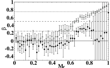
Figure 7: The distribution of the anisotropy parameter $\beta(r)$ for the simulations of class I. A plot with error-bar is the result of the numerical simulations SC with $(\bar{b_{t}},a)=(0,0)$ (gray triangle) and $(\bar{b_{t}},a)=(0.5,0)$ (black diamond) in Fig.1. A solid horizontal line represents the critical solution (16)-(20) with constant $\beta$. Each line represents the critical solution with $\beta=0$ (solid line), $0.25$ (dot-dashed line), $0.5$ (dashed line), and $0.75$ (dotted line), respectively.

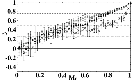
Figure 8: Same as Fig.7 but for the simulations of class II. A plot is the result of the numerical simulations SC with $(\bar{b_{t}},a)=(0,1)$ (black diamond), $(0,2)$ (gray triangle), and CC (cross) in Fig.1. Each line represents the critical solution with $\beta=0$ (solid line), $0.25$ (dot-dashed line), $0.5$ (dashed line), and $0.75$ (dotted line), respectively.

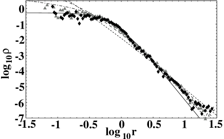
Figure 9: A log-log plot for a density profile for class I simulations with the unit of $r_{h}=M_{tot}=G=1$, where $r_{h}$ is the half-mass radius of the bound system. A plot is the result of the numerical simulations SC with $(\bar{b_{t}},a)=(0,0)$ (gray triangle) and $(\bar{b_{t}},a)=(0.5,0)$ (black diamond) in Fig.1. Each line represents the critical solution with $\beta=0$ (solid line), $0.25$ (dot-dashed line), $0.5$ (dashed line), and $0.75$ (dotted line), respectively.

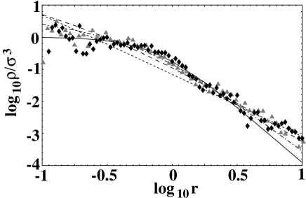
Figure 10: Phase space density for class I simulations with the unit of $r_{h}=M_{tot}=G=1$. A plot is the result of the numerical simulations SC with $(\bar{b_{t}},a)=(0,0)$ (gray triangle) and $(\bar{b_{t}},a)=(0.5,0)$ (black diamond) in Fig.1. Each line represents the critical solution with $\beta=0$ (solid line), $0.25$ (dot-dashed line), $0.5$ (dashed line), and $0.75$ (dotted line), respectively.

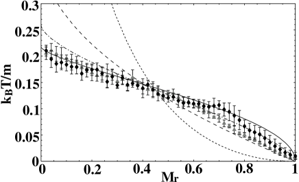
Figure 11: Temperature-Mass relations for class I simulations with the unit of $r_{h}=M_{tot}=G=1$. A plot with error-bar is the result of the numerical simulations SC with $(\bar{b_{t}},a)=(0,0)$ (gray triangle) and $(\bar{b_{t}},a)=(0.5,0)$ (black diamond) in Fig.1. Each line represents the critical solution with $\beta=0$ (solid line), $0.25$ (dot-dashed line), $0.5$ (dashed line), and $0.75$ (dotted line), respectively.

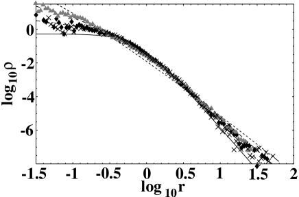
Figure 12: Same as Fig.9 but for class II simulations. A plot is the result of the numerical simulations SC with $(\bar{b_{t}},a)=(0,1)$ (black diamond), $(0,2)$ (gray triangle), and CC (cross) in Fig.1.

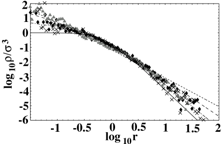
Figure 13: Same as Fig.10 but for class II simulations. A plot is the result of the numerical simulations SC with $(\bar{b_{t}},a)=(0,1)$ (black diamond), $(0,2)$ (gray triangle), and CC (cross) in Fig.1.

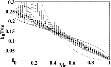
Figure 14: Same as Fig.11 but for class II simulations. A plot with error-bar is the result of the numerical simulations SC with $(\bar{b_{t}},a)=(0,1)$ (black diamond), $(0,2)$ (gray triangle), and CC (cross) in Fig.1.

Here we compare the results of these N-body simulations with those of the critical solutions in the previous section from the viewpoints of mass density, temperature-mass (TM) relation, and phase space density. In cosmological simulations, it is well known that the phase space density has a remarkable character, i.e., it has a single exponent with radius in the wide range of the viriallized region, despite the fact that the density has two different exponents Taylor01 . However, it is not obvious that it behaves in the same way for the simulations with different initial conditions. Hence it seems meaningful to examine the behavior of this quantity in our cold collapse simulations.

First we compare the numerical results in the simulations of class I with the critical solutions with constant $\beta$. The densities fit well to the distribution of the Plummer’s solution in the inner region as is shown in our previous paper (Fig.9). They, however, deviate from the Plummer’s distribution in the outer region where the velocity anisotropy is developed. We observe that the density in this region fits well rather to that of the critical solution with positive constant $\beta$. Both the TM relation and the phase space density have the same characters, i.e., both of them fit well to those of the Plummer’s solution in the inner region and to those of the positive constant $\beta$ critical solution in the outer region (Figs.10 and 11). We can also derive the analytical solution which fits well to all of these physical quantities in the full region by connecting the inner Plummer’s solution with the outer critical solution with positive constant $\beta$ (Appendix B or reference Sota05 ). The phase space density in these simulations becomes flat in the central part as well as the mass density. In the critical solution, the central part is described by the fixed point $\gamma=\gamma_{a}$, for which the exponent of the relative potential vanishes. Hence the exponent of the phase space density inevitably takes the same value as that of the mass-density at the center, as long as the phase space distribution follows the critical solution with constant $\beta$.

For the simulations of class II, the anisotropy parameter $\beta$ behaves quite differently. In those cases the velocity dispersion is anisotropic even in the inner region. Actually, the mass densities for those simulations are neither cuspy nor flat in the central region (Fig.12). Although the anisotropy parameter $\beta$ is not constant but is monotonically increasing outward, the density profiles fit well to that of the critical solutions with $\beta$=0.5 to 0.75 in full of the bound region. Both the phase space densities and TM relations for these simulations are also fitted to these critical solutions quite well, except for the case with the initial high density simulation with $(\bar{b_{t}},a)=(0,2)$.

In this last case with $(\bar{b_{t}},a)=(0,2)$, the phase space density becomes cuspy against the behavior of the mass density (Fig.13) and the temperature falls off at the center against the behavior of any critical solutions (Fig.14). These results are certainly correlated with the deviation from the LV relation at the central region. In this simulation, the kinetic energy is not sufficiently gained to attain the LV relation, which reflects both the temperature falling off and the steepness of the phase space density which is derived from dividing the density with the falling temperature.

V Conclusions and Discussions

We focused on the local virial (LV) relation and investigated the role of the LV relation in a spherically symmetric steady state system. Assuming the constant LV ratio and solving Jeans equation for spherically steady state system, we studied the full solution space of the problem under constant anisotropy parameter and obtained some meaningful solutions. Especially, if the LV relation is satisfied, the solution of the power law behavior of the density profile in both the asymptotic regions $r\rightarrow 0$ and $\infty$ exists and is commonly observed in many numerical simulations. In this sense, the LV relation plays a critical role in solutions of Jeans equation for spherically steady state system.

In the previous section, we compared our cold collapse simulations with the critical solution with constant anisotropy parameter $\beta$. We got the results that the simulations agree with the critical solutions quite well except for the initially high density simulation with $(\bar{b_{t}},a)=(0,2)$. In that simulation, the LV ratio $b$ becomes smaller than one around the center, where the temperature falls off and the phase-space density becomes steeper than the mass density.

These results remind us of the cosmological simulations for which both mass density and the phase space density have the universal characters. In the cosmological simulation, the phase space density behaves as $\rho/\sigma^{3}\sim r^{-\alpha}$, where $\alpha\sim 1.87$ Dehnen05 ; Taylor01 , which is larger than the exponent of the mass density in the central part and the temperature falls off in the central region. Hence we speculate that both of the initial high density simulations and cosmological simulations have the common characters for the phase space distribution. This may be because in the initially high density simulation, the matters in the central part collapse to make a core in the early stage and the matters in the outer part gradually falls into the core in the later stage, which is similar to the case with the secondary in-fall in the cosmological simulation.

However, we have to be careful to conclude that these results mean the inapplicability of the LV relation for these cases, because we compared these cases only under the condition $\beta$ is constant. It is not obvious that the same kind of asymptotic behavior of the critical solutions obtained under the LV relation are sustained for any function form of $\beta(r)$. We will discuss these points in our coming paper.

Appendix A A solution for $\alpha=1$ case

A.1 $\beta=1$ case

In the case for $(\beta,b)=(1,1)$, the equation (8) becomes

$$\gamma^{\prime}=(\gamma-\gamma_{+})(\gamma-\gamma_{-})=\kappa,$$ (21)

where

$$\gamma_{+}=\frac{5+\sqrt{1-4\kappa}}{2},\quad\quad\gamma_{-}=\frac{5-\sqrt{1-4\kappa}}{2}.$$ (22)

Integrating the Eq.(21), we obtain

$$\gamma=\frac{\gamma_{+}+\gamma_{-}x^{\gamma_{+}-\gamma_{-}}}{1+x^{\gamma_{+}-\gamma_{-}}},$$ (23)

where we choose the integral constant as satisfying the condition $\gamma(1)=(\gamma_{+}+\gamma_{-})/2$. At large $x$, $\gamma$ approaches $\gamma_{-}$ and the total mass is infinite because $\gamma_{-}\leq 5/2$. From Eqs.(7), (5), and (23), we have

$$\rho\propto x^{-\gamma_{+}}\left(1+x^{\gamma_{+}-\gamma_{-}}\right),$$ (24)

$$M\propto 4\pi x^{3-\gamma_{+}}\left(\frac{1}{3-\gamma_{+}}+\frac{x^{\gamma_{+}-\gamma_{-}}}{3-\gamma_{-}}\right),$$ (25)

$$\phi\propto x^{2-\gamma_{+}}\left(1+x^{\gamma_{+}-\gamma_{-}}\right),$$ (26)

$$\sigma^{2}\propto\frac{1}{2}x^{2-\gamma_{+}}\left(1+x^{\gamma_{+}-\gamma_{-}}\right),$$ (27)

$$\rho/\sigma^{3}\propto 2^{3/2}x^{\gamma_{+}/2-3}\left(1+x^{\gamma_{+}-\gamma_{-}}\right)^{-1/2},$$ (28)

where $M:=\int_{0}^{x}4\pi u^{2}\rho du$.

A.2 $\beta\neq 1$ case

In this case, the equation (8) becomes

$$\gamma^{\prime}-(\gamma-\gamma_{a})(\gamma-\gamma_{b})=\kappa x^{2(1-\beta)},$$ (29)

where

$$\gamma_{a}=2\beta,\quad\quad\gamma_{b}=2\beta+1.$$ (30)

The behavior of the solutions in Eq.(29) shows in Fig.15. In the limit $r\rightarrow 0$, $\gamma$ approaches $\gamma_{a}$ or $\gamma_{b}$ or $-\infty$ (inner hole). On the other hand, in the limit $r\rightarrow\infty$, all solutions have an outer truncation at $r=\infty$. Physically meaningful solution is represented by a solid line in Fig.15 where $\gamma$ approaches $\gamma_{a}$ at $r\rightarrow 0$.

Figure 15: The same as Fig.2, but for case $\alpha=1(\beta\neq 1)$. The parameters are set to $(\beta,b)=(3/4,3/2)$.

Appendix B the connection of relative potentials

Here we connect two critical solutions with different values of constant $\beta$, which leads to the critical solution with a step function form of $\beta\left(r\right)$. Here we use the unit $G=r_{c}=\phi_{c}=1$, where $r_{c}$ is the radius of the connected position and $\phi_{c}$ is the value of the relative potential at $r=r_{c}$. In this unit the relative potentials $\phi_{1}$ in the inner region and $\phi_{2}$ in the outer region are described as

$$\phi_{1} = \left(\frac{1+c_{1}^{s_{1}}}{r^{s_{1}}+c_{1}^{s_{1}}}\right)^{1/s_{1}},$$ (31)

$$\phi_{2} = \left(\frac{1+c_{2}^{s_{2}}}{r^{s_{2}}+c_{2}^{s_{2}}}\right)^{1/s_{2}},$$ (32)

respectively. Each potential includes a free parameter $c_{1}$ or $c_{2}$ other than the parameter $s_{1}$ and $s_{2}$ related to the anisotropy of each region. From the continuous condition of the first derivative of $\phi_{1}$ and $\phi_{2}$ against $r$ at $r=1$, $c_{2}$ is described as

$$c_{2}=c_{1}^{s_{1}/s_{2}}.$$ (33)

Hence connected solution depends on the one-parameter $c=c_{1}$ for given $s_{1}$ and $s_{2}$.

This parameter $c$ determines the mass fraction of the inner solution $\phi_{1}$ against total mass as

$$\frac{M_{1}}{M_{tot}}=\left({1+c^{s_{1}}}\right)^{-1-1/s_{2}}.$$ (34)

Hence we can adjust the mass fraction of the inner region by changing the parameter $c$.

- (1) M. Hénon, Ann. Astrophys. 27, 83 (1964).
- (2) T. S. van Albada, Mon. Not. R. Astron. Soc. 201, 939 (1982).
- (3) J. Binney and S. Tremaine, Galactic Dynamics (Princeton University Press, Princeton, 1987).
- (4) O. Iguchi, Y. Sota, T. Tatekawa, A. Nakamichi, and M. Morikawa, Phys. Rev. E 71, 016102 (2005).
- (5) Y. Sota, O. Iguchi, M. Morikawa, and A. Nakamichi, astro-ph/0403411, submitted to Phys.Rev.E, (2005).
- (6) N. W. Evans and J. An, Mon. Not. R. Astron. Soc. 360, 492 (2005).
- (7) A. Kawai, T. Fukushige, J. Makino, and M. Taiji, Publ. Astron. Soc. Japan 52, 659 (2000).
- (8) W. Dehnen and D. E. McLaughlin, Mon. Not. R. Astron. Soc. 363, 1057 (2005).
- (9) Y. Sota, O. Iguchi, M. Morikawa, and A. Nakamichi, Proceedings of CN-Kyoto International Workshop on Complexity and Nonextensivity, (2005).
- (10) Ü. -I. K. Veltmann, Astron. Zh. 56, 976 (1979).
- (11) J. E. Taylor and J. F. Navarro, ApJ. 563, 483 (2001).