The 21 centimeter Background from the Cosmic Dark Ages: Minihalos and the Intergalactic Medium before Reionization

Abstract

The H atoms inside minihalos (i.e. halos with virial temperatures $T_{\rm vir}\leq 10^{4}{\rm K}$, in the mass range roughly from $10^{4}M_{\odot}$ to $10^{8}M_{\odot}$) during the cosmic dark ages in a $\Lambda$CDM universe produce a redshifted background of collisionally-pumped 21-cm line radiation which can be seen in emission relative to the cosmic microwave background (CMB). Previously, we used semi-analytical calculations of the 21-cm signal from individual halos of different mass and redshift and the evolving mass function of minihalos to predict the mean brightness temperature of this 21-cm background and its angular fluctuations. Here we use high-resolution cosmological N-body and hydrodynamic simulations of structure formation at high redshift ($z\mathrel{\hbox{\hbox to0.0pt{\hbox{\lower 4.0pt\hbox{$\sim$}}\hss}\hbox{$>$}}}8$) to compute the mean brightness temperature of this background from both minihalos and the intergalactic medium (IGM) prior to the onset of Ly$\alpha$ radiative pumping. We find that the 21-cm signal from gas in collapsed, virialized minihalos dominates over that from the diffuse shocked gas in the IGM.

1. Introduction

One of the most promising means by which to observe the high redshift universe in the cosmic “dark ages” is through the 21-cm wavelength hyperfine transition of the neutral hydrogen that is abundant prior to reionization (e.g. Scott & Rees 1990; Subramanian & Padmanabhan 1993). Motivated by the prospect of new radio telescopes that will be able to observe such a signal, several specific observational techniques have been proposed. Among these are the angular fluctuations on the sky (e.g. Madau, Meiksin, & Rees 1997; Tozzi et al. 2000; Iliev et al. 2002 – ISFM hereafter; Ciardi & Madau 2003; Iliev et al. 2003; Zaldarriaga, Furlanetto, & Hernquist 2004; Furlanetto, Sokasian, & Hernquist 2004), features in the frequency spectrum of the signal averaged over a substantial patch of the sky (Shaver et al. 1999; Gnedin & Shaver 2004) and studies of absorption features in the spectra of bright, high-redshift radio sources (Carilli, Gnedin, & Owen 2002; Furlanetto & Loeb 2002; Martel et al. 2003).

For most of these techniques, with the exception of foreground absorption against bright radio sources, the 21-cm signal must be distinguished from the CMB, which is only possible if the 21-cm level population corresponds to a spin temperature $T_{\rm S}$, which differs from the temperature, $T_{\rm CMB}$, of the CMB. Since radiative excitation and stimulated emission of this transition by CMB photons tends to drive the value of $T_{\rm S}$ toward $T_{\rm CMB}$, some competing mechanism must exist to decouple $T_{\rm S}$ from $T_{\rm CMB}$. There are two main physical mechanisms by which the spin temperature is decoupled from the CMB temperature: “Ly$\alpha$ pumping,” or absorption of radiation with a wavelength in the Ly$\alpha$ transition, followed by decay into one of the hyperfine levels of the ground state (the “Field-Wouthuysen effect” – Wouthuysen 1952; Field 1959), and spin exchange during collisions between neutral hydrogen atoms (Purcell & Field 1956). The efficiency of Ly$\alpha$ pumping depends upon the intensity of the UV radiation field at the Ly$\alpha$ transition, whereas the efficiency of collisional coupling depends upon the local gas density and temperature.

For $z\mathrel{\hbox{\hbox to0.0pt{\hbox{\lower 4.0pt\hbox{$\sim$}}\hss}\hbox{$>$}}}150$, these mechanisms are ineffective at decoupling $T_{\rm S}$ from $T_{\rm CMB}$, since the kinetic temperature of the gas, $T_{\rm K}$, is coupled to $T_{\rm CMB}$ by inverse Compton scattering, and sources of UV radiation have not yet formed to initiate Ly$\alpha$ pumping. At $z\mathrel{\hbox{\hbox to0.0pt{\hbox{\lower 4.0pt\hbox{$\sim$}}\hss}\hbox{$<$}}}150$, however, $T_{\rm K}$ drops below $T_{\rm CMB}$ and, for $z\mathrel{\hbox{\hbox to0.0pt{\hbox{\lower 4.0pt\hbox{$\sim$}}\hss}\hbox{$>$}}}20$, gas at the mean density is sufficiently dense for collisions to couple $T_{\rm S}$ to $T_{\rm K}$. During the “dark ages,” therefore, when there is no Ly$\alpha$ pumping, the mean 21-cm signal against the CMB will be zero at $z\mathrel{\hbox{\hbox to0.0pt{\hbox{\lower 4.0pt\hbox{$\sim$}}\hss}\hbox{$>$}}}150$, then in absorption at $20\mathrel{\hbox{\hbox to0.0pt{\hbox{\lower 4.0pt\hbox{$\sim$}}\hss}\hbox{$<$}}}z\mathrel{\hbox{\hbox to0.0pt{\hbox{\lower 4.0pt\hbox{$\sim$}}\hss}\hbox{$<$}}}150$.

At lower redshift, collisions become negligible for gas at or below the cosmic mean density, and such gas becomes invisible until its spin temperature is again decoupled from the CMB by Ly$\alpha$ pumping due to an early UV background from the first stars and quasars. Even though collisional decoupling is ineffective for $z\mathrel{\hbox{\hbox to0.0pt{\hbox{\lower 4.0pt\hbox{$\sim$}}\hss}\hbox{$<$}}}20$ for gas at the mean density, gas in overdense and/or heated regions can still be collisionally-decoupled. In particular, the gas density within “minihalos” – virialized halos of dark and baryonic matter with masses $10^{4}\mathrel{\hbox{\hbox to0.0pt{\hbox{\lower 4.0pt\hbox{$\sim$}}\hss}\hbox{$<$}}}M\mathrel{\hbox{\hbox to0.0pt{\hbox{\lower 4.0pt\hbox{$\sim$}}\hss}\hbox{$<$}}}10^{8}M_{\sun}$ and virial temperatures $T<10^{4}K$ which are too low to collisionally ionize their H atoms – is sufficiently high so as to decouple its gas spin temperature from the CMB, with $T_{\rm S}>T_{\rm CMB}$ in general, causing it to appear in emission (ISFM). ISFM predicted the mean and angular fluctuations of the corresponding 21-cm signal by a semi-analytical calculation which integrated the equation of transfer through individual minihalos of different mass at different redshifts ($z>6$) and summed these individual halo contributions over the evolving statistical distribution of minihalo masses in the $\Lambda$CDM universe. Iliev et al. (2003) extended these results to include non-linear biasing effects. These authors concluded that the fluctuations in intensity across the sky created by minihalos were likely to be observable by the next generation of low-frequency radio telescopes. Such observations could confirm the basic CDM paradigm and constrain the shape and amplitude of the power spectrum at much smaller scales than previously possible.

Since then, Furlanetto & Loeb (2004) have suggested that shocked, overdense gas in the diffuse IGM (prior to the onset of Ly$\alpha$ radiative pumping) is also capable of producing a 21-cm emission signal and that this IGM contribution to the mean signal will dominate over that from gas inside minihalos. Their conclusion is based on an extension of the Press-Schechter approximation (Press & Schechter 1974) that is used to determine the fraction of baryons in the diffuse IGM that are hot and dense enough to produce a 21-cm emission signal. We will address this question here.

In order to quantify these effects, we have computed the 21-cm signal both from minihalos and the IGM at $z\mathrel{\hbox{\hbox to0.0pt{\hbox{\lower 4.0pt\hbox{$\sim$}}\hss}\hbox{$>$}}}8$ for the first time using high-resolution cosmological N-body and hydrodynamic simulations of structure formation. We have assumed a flat, $\Lambda$CDM cosmology with matter density parameter $\Omega_{m}=0.27$, cosmological constant $\Omega_{\Lambda}=0.73$, baryon density $\Omega_{b}=0.043$, Hubble constant $H={\rm 70\,km\,s^{-1}Mpc^{-1}}$, linearly-extrapolated $\sigma_{8h^{-1}}=0.9$ and the “untilted” Harrison-Zel’dovich primordial power spectrum.

In this paper, we present detailed, high-resolution gas and N-body simulations which predict the 21-cm signal at $z>6$ due to collisional decoupling from the CMB before the UV background is strong enough to make decoupling due to Ly$\alpha$ pumping important. Because the Ly$\alpha$ pumping efficiency is expected to fluctuate strongly until enough sources form to make the efficiency uniform (e.g. Barkana & Loeb 2004), the results presented here will also be relevant for isolated patches of the universe during reionization itself, which would depend upon the location and abundance of the first sources of UV radiation. Within such regions, we focus on properly resolving the gasdynamics of structure formation at small scales through the use of high resolution gasdynamic and N-body simulations. We test the semi-analytical prediction of the halo model of ISFM for the contribution to the mean signal from gas in minihalos, and investigate the extent to which IGM gas may provide a non-negligible contribution to the total fluctuating signal, as suggested by Furlanetto & Loeb (2004).

These results were first summarized in Ahn et al. (2006). Here we shall describe our calculations in full and present our results in more detail.

The outline of this paper is as follows. In § 2 we summarize the basic physics of the 21-cm emission and absorption and the analytical model of ISFM. We also describe our cosmological simulations and their initial conditions, and our method for obtaining the 21-cm signal from our simulations. In § 3 we present our results. Our conclusions are summarized in § 4.

2. The Calculation

2.1. Physics of 21-cm signal from neutral hydrogen

The hyperfine splitting of the ground state of hydrogen leads to a transition with excitation temperature $T_{*}=0.068\,{\rm K}$, wavelength $\lambda_{0}=21.16\,{\rm cm}$, and frequency $\nu_{0}=1.417\,{\rm GHz}$. The ratio of populations of the upper ($n_{1}$) and lower ($n_{0}$) states is characterized by the spin temperature $T_{\rm S}$ according to

$$\frac{n_{1}}{n_{0}}=3\exp\left(-T_{*}/T_{\rm S}\right).$$ (1)

Neutral hydrogen at redshift $z$ produces a differential signal relative to the CMB at redshifted wavelength $21(1+z)\,{\rm cm}$ only if $T_{\rm S}$ differs from $T_{\rm CMB}$. The $21\,{\rm cm}$ transition is seen in emission against the CMB if $T_{\rm S}>T_{\rm CMB}$ or in absorption if $T_{\rm S}<T_{\rm CMB}$. The value of $T_{\rm S}$ is determined by the relative importance of collisional and radiative excitations. A hydrogen atom can 1) absorb a 21-cm photon from the CMB (CMB pumping), 2) collide with another atom (collisional pumping) and 3) absorb a Ly$\alpha$ photon to make a Ly$\alpha$ transition, then decay to one of the hyperfine 21-cm levels (Ly$\alpha$ pumping). These pumping mechanisms jointly determine the spin temperature,

$$T_{S}=\frac{T_{{\rm CMB}}+y_{\alpha}T_{\alpha}+y_{\rm c}T_{\rm K}}{1+y_{\alpha}+y_{\rm c}},$$ (2)

where $T_{\alpha}$ is the color temperature of the Lyman-$\alpha$ photons, $T_{\rm K}$ is the kinetic temperature, $y_{\alpha}$ is the Lyman-$\alpha$ coupling constant, and $y_{\rm c}$ is the collisional coupling constant (Purcell & Field 1956; Field 1959). As seen in equation (2), the spin temperature deviates from $T_{\rm CMB}$ only when these couplings exist. Throughout this paper, we will consider only the collisionally coupled gas, or the case where $y_{\alpha}=0$. This is valid when 1) light sources were not yet abundant enough to build up substantial Lyman-$\alpha$ background or 2) the region of interest is far enough away from light sources. The collisional coupling constant is given by

$$y_{\rm c}=\frac{T_{*}C_{10}}{T_{\rm K}A_{10}},$$ (3)

where $A_{10}=2.85\times 10^{-15}{\rm s}^{-1}$ is the Einstein spontaneous emission coefficient, and $C_{10}=\kappa(1-0)n_{\rm H}$ is the atom-atom collisional de-excitation rate (Purcell & Field 1956). We use $\kappa(1-0)$ tabulated in Zygelman (2005) which is valid for $1{\rm K}<T_{\rm K}<300{\rm K}$, and for higher $T_{\rm K}$ we use $\kappa(1-0)$ tabulated in Allison & Dalgarno (1969).

The 21-cm line can be observed in either absorption or emission against the CMB, with a differential brightness temperature defined by

$$\delta T_{b}(\nu)\equiv T_{b}(\nu)-T_{\rm CMB,0},$$ (4)

where $T_{b}(\nu)$ is the brightness temperature at an observed frequency $\nu$ and $T_{\rm CMB,0}$ is the present-day CMB temperature. $T_{b}(\nu)$ satisfies the radiative transfer equation in the Rayleigh-Jeans limit,

$$T_{b}(\nu)=T_{\rm CMB,0}e^{-\tau_{\nu}}+\int_{0}^{\tau_{\nu}}d\tau^{\prime}_{\nu^{\prime}}\frac{T_{\rm S}(z^{\prime})}{1+z^{\prime}}e^{-(\tau_{\nu}-\tau^{\prime}_{\nu^{\prime}})},$$ (5)

where $\tau_{\nu}=\int_{0}^{\tau_{\nu}}d\tau^{\prime}_{\nu^{\prime}}$ is the 21-cm optical depth of the neutral hydrogen atoms to photons in the CMB observed today at frequency $\nu$, $\tau^{\prime}_{\nu^{\prime}}=\int_{0}^{\tau^{\prime}_{\nu^{\prime}}}d\tau^{\prime\prime}_{\nu^{\prime\prime}}$ is the optical depth of the neutral hydrogen atoms at redshift $z^{\prime}$ to photons at a frequency $\nu^{\prime}=\nu(1+z^{\prime})$ (the frequency which a comoving observer sees at redshift $z^{\prime}$), $T_{\rm S}(z^{\prime})$ is the spin temperature of intervening gas located at redshift $z^{\prime}$, and the infinitesimal optical depth along the path of the photon as it travels for cosmic time interval $dt^{\prime}$ is given by

$$d\tau^{\prime}_{{\nu^{\prime}}} = c\,dt^{\prime}\,\kappa_{\nu^{\prime}}(\nu^{\prime},z^{\prime})$$ (6)

$$= \left[\frac{c\,dz^{\prime}}{H(z^{\prime})(1+z^{\prime})}\right]\left[\frac{3c^{2}A_{10}n_{\rm HI}(z^{\prime})}{32\pi{\nu^{\prime}}^{2}}\phi(\nu^{\prime})\frac{T_{*}}{T_{\rm S}(z^{\prime})}\right],$$

where $H(z)$ is the Hubble constant at redshift $z$, and $n_{\rm HI}$ is the local density of neutral hydrogen. The line profile $\phi(\nu^{\prime})$ satisfies

$$\int_{-\infty}^{+\infty}d\nu^{\prime}\phi(\nu^{\prime})=1,$$ (7)

and is in a general form. For instance, in the presence of both thermal Doppler broadening and the Doppler shift due to peculiar motion, the line profile is given by

$$\phi(\nu^{\prime})=\frac{1}{\Delta\nu^{\prime}\sqrt{\pi}}\exp\left[-\frac{(\nu^{\prime}-\nu^{\prime}_{0})^{2}}{{\Delta\nu^{\prime}}^{2}}\right],$$ (8)

where $\Delta\nu^{\prime}=(\nu^{\prime}_{0}/c)\sqrt{2kT/m}$, and the Doppler-shifted line center is given by

$$\nu^{\prime}_{0}=\nu_{0}\frac{1+\beta}{\sqrt{1-\beta^{2}}},$$ (9)

where $\beta={\rm v}/c$ is the line-of-sight peculiar velocity of gas (in units of the speed of light) toward the observer.

2.1.1 The unperturbed universe

Figure 1.— Analytical prediction for the mean 21-cm differential brightness temperature due to collisionally-decoupled minihalos and an unperturbed IGM. Shown are the results based on the Press-Schechter (solid) and the Sheth-Tormen (dotted) mass functions for halos and the contribution from IGM gas with cosmic mean density and temperature (dashed). In the bottom panel, we show the minihalo collapsed fraction in the $\Lambda$CDM universe, again based on the Press-Schechter (solid) and the Sheth-Tormen (dotted) mass functions.

Solutions to the general radiative transfer equation (eq. [5]) exist in simplified forms in limiting cases. If the line is un-broadened and un-shifted, i.e. $\phi(\nu^{\prime})=\delta(\nu^{\prime}-\nu_{0})$, the solution to equation (5) becomes

$$T_{b}(\nu)=T_{\rm CMB,0}e^{-\tau(z)}+\frac{T_{\rm S}(z)}{1+z}\left[1-e^{-\tau(z)}\right],$$ (10)

where $\nu$ and $z$ satisfy $\nu_{0}=\nu(1+z)$, and

$$\tau(z)\equiv\frac{3\lambda_{0}^{3}A_{10}T_{*}n_{\rm HI}(z)}{32\pi T_{S}H(z)}=3.22\times 10^{-3}$$

$$\times\left(\frac{\Omega_{b}h^{2}}{0.0224}\right)\left(\frac{\Omega_{0}h^{2}}{0.135}\right)^{-0.5}\left(\frac{T_{\rm CMB}}{T_{\rm S}}\right)(1+z)^{0.5},$$ (11)

using $n_{\rm HI}=x_{\rm HI}n_{\rm H}$ , where $n_{\rm H}=1.9\times 10^{-7}{\rm cm}^{-3}(1+z)^{3}$ and $x_{\rm HI}$ is the neutral fraction of hydrogen. The IGM kinetic temperature, $T_{\rm K}$, is coupled to $T_{\rm CMB}$ by Compton scattering at $z\mathrel{\hbox{\hbox to0.0pt{\hbox{\lower 4.0pt\hbox{$\sim$}}\hss}\hbox{$>$}}}134$. For $z\mathrel{\hbox{\hbox to0.0pt{\hbox{\lower 4.0pt\hbox{$\sim$}}\hss}\hbox{$<$}}}100$, the kinetic temperature of the unperturbed gas in the $\Lambda$CDM universe is well approximated by

$$T_{\rm K} \approx T_{\rm CMB}(z=134){(1+z)^{2}}/{(1+134)^{2}}$$ (12)

$$= 368.55{\rm K}\times{(1+z)^{2}}/{(1+134)^{2}}.$$

Since $T_{\rm CMB}/T_{\rm S}<{\rm max}\{1,\,T_{\rm CMB}/T_{\rm K}\}$, in general, $\tau_{\nu}\ll 1$ for the unperturbed IGM at all redshifts of interest ($8\mathrel{\hbox{\hbox to0.0pt{\hbox{\lower 4.0pt\hbox{$\sim$}}\hss}\hbox{$<$}}}z\mathrel{\hbox{\hbox to0.0pt{\hbox{\lower 4.0pt\hbox{$\sim$}}\hss}\hbox{$<$}}}50$), as seen in equation (2.1.1). In that case, equation (10) can be approximated as

$$\delta T_{b}(\nu)=\left[T_{\rm S}(z)-T_{\rm CMB}(z)\right]\tau(z)/(1+z)$$ (13)

using equation (4). We can use equations (2.1.1) and (13) to describe the signal from the unperturbed gas in the Universe, because the line profile in this case is narrow enough to be approximated by a Dirac-$\delta$ function. With equations (2), (3), (2.1.1) and (13), one can calculate $\delta T_{b}$ of the unperturbed gas of the Universe, well approximated by

$$\delta T_{b}(z)\approx-10\,{\rm mK}\frac{F[\log_{10}(1+z)]}{F[\log_{10}(1+36.8)]}\,,$$ (14)

where

$$F(x)={\rm dex}(3172.36-18037.3\,x+43430.3\,x^{2}-57481.7\,x^{3}$$

$$+45150.0\,x^{4}-21042.1\,x^{5}+5388.50\,x^{6}-585.165\,x^{7}),$$ (15)

which is in absorption until collisional pumping becomes negligible at $z\simeq 20$ (Fig. 1; see also Bharadwaj & Ali 2004 and Zygelman 2005).

2.1.2 Perturbed universe: optically thin case

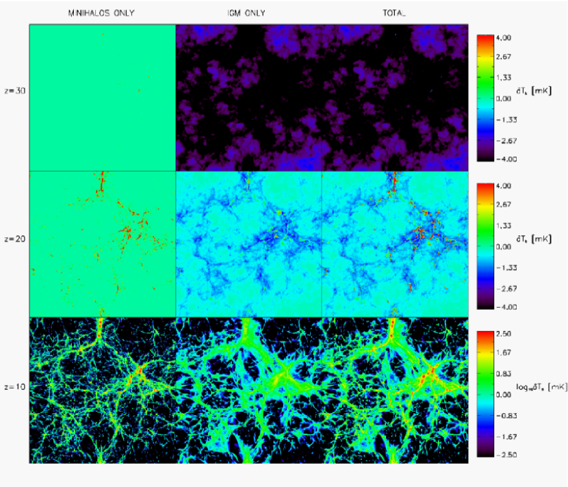
Figure 2.— Map of the differential brightness temperature, $\delta T_{b}$, (projected onto one surface of the box) for the redshifted 21-cm signal obtained from our highest resolution simulation, C4. Rows, top to bottom, show redshifts $z$=30, 20, and 10. Columns, left to right, represent contributions from minihalos, the IGM and the total signal. Note that the scale is linear in $\delta T_{b}$ for the upper two rows of images, but logarithmic for the bottom row.

Thermal Doppler broadening and Doppler shift by peculiar motions would drive $\phi$ to be broadened and shifted, causing overlap of line profiles. In such cases, the solution to equation (5), in general, is not given in a simple form as in equation (10). We show here, however, that the simple solution given by equation (13) also applies to the overlapped line profile case, as long as the optical depths, both infinitesimal and integrated, of gas in the simulation box are small. In such optically-thin limit, equation (5) can be approximated as

$$T_{b}(\nu)=T_{\rm CMB,0}(1-\tau_{\nu})+\int_{0}^{\tau_{\nu}}d\tau^{\prime}_{\nu^{\prime}}\frac{T_{\rm S}(z^{\prime})}{1+z^{\prime}}.$$ (16)

The differential brightness temperature from a simulation box at $z$ with a redshift-spread $\Delta z$ ($\ll z$) and angle-spread $\Delta\Omega$ is

$$\overline{\delta T}_{b}(\nu)\equiv\frac{\int d\nu d\Omega\,\delta T_{b}(\nu)}{\int d\nu d\Omega},$$ (17)

where the frequency and angle intervals of integration are set by the size of the box. As the angle integration is a simple sum of different line-of-sight contributions which do not interfere with each other, we can first perform the line-of-sight average,

$$\left.\overline{\delta T}_{b}(\nu)\right|_{\rm l.o.s.}=\frac{\int^{\nu+\delta\nu/2}_{\nu-\delta\nu/2}d\nu\,\delta T_{b}(\nu)}{\int^{\nu+\delta\nu/2}_{\nu-\delta\nu/2}d\nu},$$ (18)

and then integrate over angles. In equation (18), one can show that

$$\int^{\nu+\delta\nu/2}_{\nu-\delta\nu/2}d\nu=\frac{\nu_{0}}{(1+z)^{2}}\int^{z+\Delta z/2}_{z-\Delta z/2}dz^{\prime},$$ (19)

and

$$\int^{\nu+\delta\nu/2}_{\nu-\delta\nu/2}d\nu\int^{\tau_{\nu}}_{0}d\tau^{\prime}_{\nu^{\prime}}$$

$$=\frac{c\nu_{0}^{-2}}{H(z)(1+z)^{2}}\int^{z+\Delta z/2}_{z-\Delta z/2}dz^{\prime}\frac{3c^{2}A_{10}n_{\rm HI}(z^{\prime})T_{*}}{32\pi T_{\rm S}(z^{\prime})},$$ (20)

where we have used the fact that $\int_{-\infty}^{\infty}d\nu^{\prime}\phi(\nu^{\prime})=1$, and have also assumed that the thermal broadening and the Doppler shift by peculiar motions are negligible compared to the width of the box: $(\Delta\nu^{\prime})_{\rm thermal}\ll\Delta\nu^{\prime}_{\rm box}$, $(\Delta\nu^{\prime})_{\rm peculiar}\ll\Delta\nu^{\prime}_{\rm box}$. Using equations (16), (19), and (2.1.2), we then obtain

$$\left.\overline{\delta T}_{b}(\nu)\right|_{\rm l.o.s.}=\int^{\Delta z}dz^{\prime}\left(\frac{T_{\rm S(z^{\prime})}}{1+z^{\prime}}-T_{\rm CMB,0}\right)\tau(z^{\prime})\bigg{/}\int^{\Delta z}dz^{\prime},$$ (21)

which is simply an averaged superposition of contributions of gas given by equation (13), along the line-of-sight.

We have shown, in this section, that the 21-cm differential brightness temperature $\overline{\delta T}_{b}(\nu)$ can be calculated by a simple average of individual contributions from gas at different locations in a simulation box, as long as optical depths are small (eq. [21]). Care needs to be taken, however, when gas achieves considerable optical depth. In § 2.1.3, we describe how one can calculate the signal from optically-thick media, which are mostly located inside minihalos.

Figure 3.— Volume-weighted probability distribution functions (PDFs) of gas density ($1+\delta$) and differential brightness temperature ($\delta T_{b}$) for C4 versus $(1+\delta)$ and $\delta T_{b}$, respectively, for the total gas (solid), MH gas (dashed), and IGM gas (dotted). Also shown are the cumulative differential brightness temperatures, i.e. $\left<\delta T_{b}(<[1+\delta])\right>$ and $\left<\delta T_{b}(<\delta T_{b})\right>$. The top and bottom panels from left to right correspond to $z$=10, 20, and 30, respectively.

2.1.3 Perturbed universe: minihalos

Minihalos which start to emerge at $z\simeq 20$ have temperature and density high enough to produce a significant emission signal (ISFM). As the optical depth through each minihalo is not negligible, the full radiative transfer equation (eq. [5]) should be solved through individual minihalos. Once individual halo contribution $\Delta\nu_{\rm eff}\delta T_{b,\nu_{0}}$ is obtained for each given halo mass $M$, one can calculate $\overline{\delta T}_{b}$ from all the minihalos at redshift $z$ by integrating over the halo mass function $dn/dM$:

$$\overline{\delta T}_{b}=\frac{c(1+z)^{4}}{\nu_{0}H(z)}\int_{M_{{\rm min}}}^{M_{{\rm max}}}\Delta\nu_{{\rm eff}}\delta T_{b,\,\nu_{0}}A\frac{dn}{dM}dM,$$ (22)

where $\Delta\nu_{{\rm eff}}$, $\delta T_{b,\,\nu_{0}}$, and $A$ refer to the parameters of the individual virialized halo, $\Delta\nu_{{\rm eff}}=\Delta\nu^{\prime}(1+z)^{-1}=(\nu^{\prime}_{0}/c)\sqrt{2kT/m}(1+z)^{-1}$, $\delta T_{b,\,\nu_{0}}$ is the face-averaged differential brightness temperature at line center, and $A$ is the projected surface area of the halo. ISFM based their calculation on the nonsingular, truncated isothermal sphere (TIS) model for CDM halos by Shapiro, Iliev, & Raga (1999) and Iliev & Shapiro (2001), in which the halo density profile and virial temperature are fully specified by the halo mass and redshift, and the Press-Schechter (1974) mass function, which determines the number density of halos at a given redshift. The minimum minihalo mass $M_{{\rm min}}$ is set by the Jeans mass

$$M_{{\rm J}}=5.7\times 10^{3}\left(\frac{\Omega_{m}h^{2}}{0.15}\right)^{-1/2}\left(\frac{\Omega_{b}h^{2}}{0.02}\right)^{-3/5}\left(\frac{1+z}{10}\right)^{3/2}M_{\sun}.$$ (23)

For $M_{{\rm max}}$, ISFM used the mass for which the virial temperature is $10^{4}{\rm K}$:

$$M_{{\rm max}}=3.95\times 10^{7}\left(\frac{\Omega_{m}h^{2}}{0.15}\right)^{-1/2}\left(\frac{1+z}{10}\right)^{-3/2}M_{\sun}.$$ (24)

The neutral baryonic fraction of halos with mass above $M_{{\rm max}}$ is uncertain, because hydrogen will be partially ionized due to collisions and photoionization by internal sources. Thus, the mass range from $M_{{\rm min}}$ to $M_{{\rm max}}$ naturally defines the mass range of minihalos which are fully neutral. Figure 1 depicts the predicted signals from unperturbed gas as well as from minihalos. We show results for both the Press-Schechter and the Sheth-Tormen mass functions (Sheth & Tormen 2002).

2.2. Numerical Simulations

We have run series of cosmological N-body and gasdynamic simulations to derive the effect of gravitational collapse and the hydrodynamics on the predicted 21 cm signal from high redshift. Our computational box has a comoving size of $0.5\,h^{-1}\,{\rm Mpc}$, which is optimal for adequately resolving both the minihalos and the small-scale structure-formation shocks. We used the code described in Ryu et al. (1993), which uses the particle-mesh (PM) scheme for calculating the gravity evolution and an Eulerian total variation diminishing (TVD) scheme for hydrodynamics. We generated our initial conditions for the gas and dark matter distributions using the publicly available software COSMICS (Ma & Bertschinger 1995). The N-body/hydro code uses an $N^{3}$ grid and $(N/2)^{3}$ dark matter particles. In order to check the convergence of our results we ran simulations at different spatial resolutions, with grid sizes $128^{3}$, $256^{3}$, $512^{3}$, and $1024^{3}$, which we denote by C1, C2, C3, and C4, respectively. We report our results in § 3 based on our highest-resolution simulation C4 and discuss the convergence of the results in § 3.3.

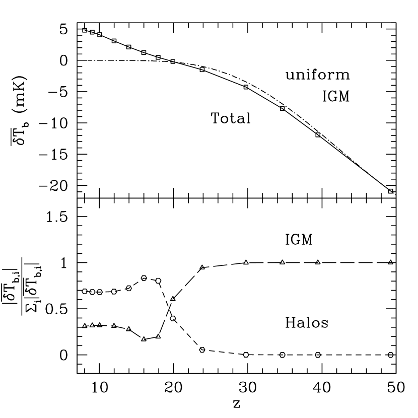
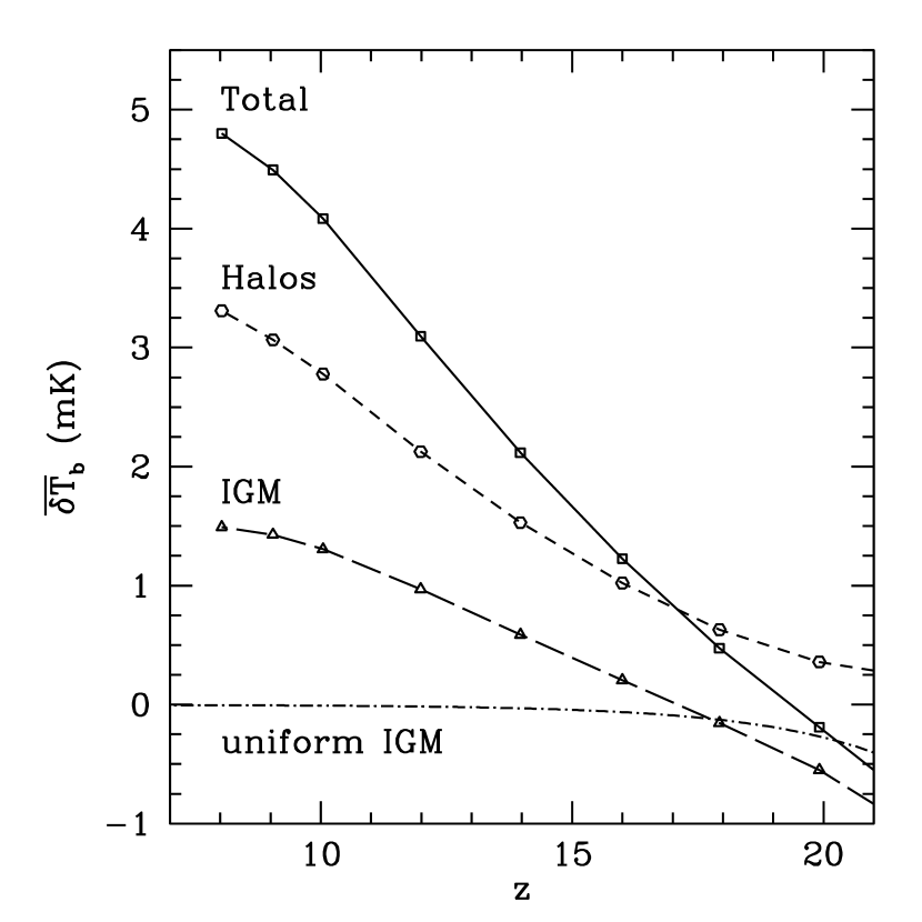
Figure 4.— Evolution of mean differential brightness temperature, $\overline{\delta T}_{b}$, of 21-cm background. (a)(left) Evolution of the total 21-cm signal vs. redshift. All data points are directly calculated from our highest resolution (C4) simulation box, with the assumption that optical depth is negligible throughout the box. (b)(right) $\overline{\delta T}_{b}$ vs. redshift below $z=20$. The contributions from minihalos (circles), the IGM (triangles), and the total (squares) are plotted, as labelled. For comparison, the result for the unperturbed IGM is also plotted (dashed-dot curves).

After the decoupling of CMB photons from the baryonic gas, the IGM gas cools adiabatically due to cosmic expansion (eq. [12]). Equation (12) agrees, for instance, with the solution to the equation (1) in Bharadwaj & Ali (2004) which describes how $T_{\rm gas}$ evolves exactly. This temperature, $T_{{\rm gas}}(z)$, was used in the simulation to set the minimum temperature of baryonic gas, to avoid negative temperatures. If a gas cell is cooled below $T_{{\rm gas}}(z)$, its temperature is set back to $T_{{\rm gas}}(z)$. Such a temperature “floor” may overestimate the gas temperature of underdense regions, but because of their low density and temperature, $y_{c}$ is small in these regions. This implies that the spin temperature $T_{\rm S}$ would be very close to $T_{\rm CMB}$, and their contribution to $\delta T_{b}$ would also be negligible, whether the kinetic temperature $T_{\rm K}$ is calculated accurately or not.

In addition to the total 21-cm signal from our simulations, $\overline{\delta T}_{b,\,{\rm IGM}}$, we are also interested in the relative contribution of the virialized minihalos and the IGM to the total signal, the sum of which gives the total 21-cm signal, $\overline{\delta T}_{b,\,{\rm tot}}=\overline{\delta T}_{b,\,{\rm halo}}+\overline{\delta T}_{b,\,{\rm IGM}}$. First, we calculate the total mean signal as a simple average over the simulation cells, $\overline{\delta T}_{b,\,{\rm tot}}\equiv{\sum_{i}\delta T_{b,\,i}}/N^{3}$. The minihalo contribution is given by $\overline{\delta T}_{b,\,{\rm halo}}\equiv{\sum_{i}f_{i}\delta T_{b,\,i}}/N^{3}$, where $f_{i}$ is the fraction of the DM mass in a cell $i$ which is part of a halo. The IGM contribution can then be obtained as

$$\overline{\delta T}_{b,\,{\rm IGM}}=\overline{\delta T}_{b,\,{\rm tot}}-\overline{\delta T}_{b,\,{\rm halo}}={\displaystyle\sum_{i}(1-f_{i})\delta T_{b,\,i}}/N^{3}.$$ (25)

In order to calculate the minihalo contribution to the total differential brightness temperature, $\overline{\delta T}_{b,\,{\rm halo}}$, one needs to first identify the halos in the simulation volume. We identified the halos using a friends-of-friends (FOF) algorithm (Davis et al. 1985) with a linking length parameter of $b=0.25$. The FOF algorithm applies to the dark matter N-body particles, rather than the gas in grid cells. Once this halo catalogue is processed for each time-slice of our N-body results, the baryonic component of each halo is identified for the grid cells of the hydrodynamics simulation which are contained within the volume of the halos in our FOF catalogue. We do this as follows. First, the density in each cell contributed by each DM particle is determined by the triangular-shaped cloud assignment scheme. For each cell in which mass is contributed by the DM particles of a given halo, the gaseous baryonic component in that cell is assumed to contribute a fraction $f_{i}$ of its mass given by the fraction of the total DM mass in that cell which is attributed to the halo DM particles. Accordingly, each cell $i$ contributes an amount $f_{i}\delta T_{{b},i}$ to the signal attributed to halo gas, while $(1-f_{i})\delta T_{{b},i}$ is assumed to be the signal from the IGM outside of the halo, where $\delta T_{{b},i}$ is calculated from the cell as a whole.

Figure 5.— Semi-analytical minihalo signal vs. IGM signal. The 21-cm flux from each halo in the simulation is found by modeling the internal structure and 21-cm line transfer through individual halos as described by ISFM (§ 2.2.1), to calculate the halo 21-cm signal from each halo more accurately. Same notation as in Figure 4. The semi-analytical 21-cm minihalo emission is higher than the raw simulated minihalo signal in Figure 4. The IGM signal remains the same. The raw minihalo and total signals plotted in Figure 4 (thin lines and open symbols) are also shown for comparison.

2.2.1 Semi-Analytical Calculation of the Halo Contribution

Our numerical simulations have sufficiently high resolution to find all halos in the computational box and the large-scale structure formation shocks, but not to resolve the internal structure of the minihalos themselves. However, as ISFM have shown, in order to obtain the correct 21-cm signal from minihalos one needs to do a full radiative transfer calculation through each individual minihalo density profile since, unlike the IGM gas, minihalos have a non-negligible optical depth at the 21-cm line. Hence, we can refine our estimate of the minihalo contribution to the total 21-cm signal by combining our numerical halo catalogers with the semi-analytic calculation of individual minihalo contribution as found by ISFM. In their approach, as described in § 2.1.3, the gas density of each minihalo is assumed to follow a TIS profile (Iliev & Shapiro 2001), radiative transfer calculations are performed to determine the $\delta T_{b}$ for different impact parameters, and, finally, the face-averaged $\delta T_{b}$ is calculated (see ISFM, for details). The halo mass function, $dn/dM$, is provided by the halo catalogue we construct from the simulation. Each individual halo contribution, $\Delta\nu_{{\rm eff}}\delta T_{b,\,\nu_{0}}A$, depends on its mass and redshift of formation (ISFM). Once we calculate $\Delta\nu_{{\rm eff}}\delta T_{b,\,\nu_{0}}A$, we then obtain the halo contribution using equation (22).

3. Results

3.1. Numerical 21-cm Brightness Temperature from Minihalos vs. IGM

In this section, we describe the results from our simulations. In Figure 2 we show (unfiltered) maps of the differential brightness temperature obtained directly from our numerical data for our highest-resolution simulation (C4), as described in § 2. We show the total signal, as well as the separate contributions from minihalos and IGM, derived as we described in § 2.2, at redshifts $z=30$, 20, and 10. At $z=30$, the earliest redshift shown (top row), most of the diffuse IGM gas is still in the quasi-linear regime and cold, thus largely in absorption against the CMB. At redshift $z=20$ (middle row), the diffuse gas is still largely in absorption, while the (relatively few) halos that have already collapsed are strongly in emission. The combination of the two contributions creates a complex, patchy emission/absorption map, and absorption and emission partially cancel each other in the total mean signal. Finally, at $z=10$ (bottom row), including its diffuse component, gas heated above $T_{\rm CMB}$ is widespread leading to a net emission against the CMB. The bulk of this 21-cm emission comes from the high-density knots and filaments. Although both the halo and IGM contributions come from roughly the same regions, the minihalo emission is significantly more clustered, while the IGM emission is quite diffuse.

In Figure 3, we have plotted the volume-weighted probability distribution functions (PDFs) for the gas density $(1+\delta)$ and the differential brightness temperature contributions $\delta T_{b}$ as functions of each other. The PDFs for gas density show that, while the highest overdensities ($\delta\mathrel{\hbox{\hbox to0.0pt{\hbox{\lower 4.0pt\hbox{$\sim$}}\hss}\hbox{$>$}}}30$) are typically found inside minihalos and the lower overdensities ($\delta\mathrel{\hbox{\hbox to0.0pt{\hbox{\lower 4.0pt\hbox{$\sim$}}\hss}\hbox{$<$}}}30$) and underdensities ($\delta\mathrel{\hbox{\hbox to0.0pt{\hbox{\lower 4.0pt\hbox{$\sim$}}\hss}\hbox{$<$}}}0$) are typically associated with the IGM, there is some overlap of the distributions for these two components. A small fraction of the volume contains lower density minihalo gas and higher density IGM gas. However, the cumulative distributions show that these volumes hardly affect the total mean brightness temperature contributed by each component. Similarly, the PDFs for the brightness temperature show that, while the volume which contributes the highest brightness temperatures is predominantly inside minihalos and that which contributes the lower brightness temperatures is predominantly located in the IGM, there is, once again, some overlap of the PDFs. A small part of the IGM volume exhibits high brightness temperature, while a small part of the minihalo volume shows low brightness temperature. Once again, however, the cumulative distributions show that these regions hardly affect the total mean brightness temperatures contributed by each component.

In Figure 4, we quantify the relative contributions of the minihalos and diffuse IGM to the total mean 21-cm signal averaged over the whole computational box and their evolution. The evolution roughly follows the naive analytical estimates, as was shown in Figure 1. The total signal is deep in absorption, with $\delta T_{b}<-10$ mK at $z>37$. The 21-cm signal is completely dominated by the IGM contribution at this stage. The absorption signal follows the analytical prediction for the unperturbed universe in § 2.1.1 well, since the density fluctuations are still small and the uniform-density assumption is reasonably accurate. The absorption continually decreases as significant nonlinear structures start forming and portions of the gas became heated due to this structure formation. The net signal goes into emission after redshift $z\sim 20$, reaching up to $\sim 5$ mK by $z\approx 8$. The emission signal at $z<18$ is due to both collapsed halos and the clumpy, hot IGM gas. In terms of their relative contributions, the minihalos dominate over the diffuse IGM at all times when the overall signal is in emission, below $z=18$. We find that the relative contributions to the total signal, $\left|\overline{\delta T}_{b,\,j}\right|/\left(\left|\overline{\delta T}_{b,\,{\rm halo}}\right|+\left|\overline{\delta T}_{b,\,{\rm IGM}}\right|\right)$ where $j$ means either “halo” or “IGM,” is nearly constant over two different redshift regimes: for $z>20$, $\left|\overline{\delta T}_{b,\,{\rm IGM}}\right|/\left(\left|\overline{\delta T}_{b,\,{\rm halo}}\right|+\left|\overline{\delta T}_{b,\,{\rm IGM}}\right|\right)\approx 1$, while for $z<16$, $\left|\overline{\delta T}_{b,\,{\rm halo}}\right|/\left(\left|\overline{\delta T}_{b,\,{\rm halo}}\right|+\left|\overline{\delta T}_{b,\,{\rm IGM}}\right|\right)\approx\,0.7$. In the transition region, $16\mathrel{\hbox{\hbox to0.0pt{\hbox{\lower 4.0pt\hbox{$\sim$}}\hss}\hbox{$<$}}}z\mathrel{\hbox{\hbox to0.0pt{\hbox{\lower 4.0pt\hbox{$\sim$}}\hss}\hbox{$<$}}}20$ the relative contributions exhibit more complex behavior, approximately canceling each other out, resulting in a total signal which is close to zero.

3.2. Refined Estimate of the Simulated Minihalo 21-cm Signal

As we discussed in § 2.2.1, we can improve our purely numerical estimate of the minihalo 21-cm signal by replacing each halo’s flux with the value obtained by detailed radiative transfer calculations. We obtain the total minihalo signal from equation (22), with the theoretical mass function $dn/dM$ replaced by the actual, numerical halo catalogue obtained from our simulations, and the individual minihalo contributions, $\Delta\nu_{{\rm eff}}\delta T_{b,\,\nu_{0}}A$, calculated by modeling each halo as a TIS.

Figure 6.— A comparison of analytical and numerical minihalo results. (a)(top) Differential brightness temperature of the 21-cm signal from minihalos for semi-analytical model (dotted: with Press-Schechter mass function; dashed: with Sheth-Tormen mass function), simulation C4 numerical result (squares) and semi-analytical calculation (§ 2.2.1) based upon simulation C4 mass function (triangles). (b)(bottom) Minihalo collapse fraction from simulation C4 (squares) and analytical mass functions (line types follow those of the top panel).

Figure 7.— Numerical resolution convergence results. Mean differential brightness temperature signals for simulations C1 (squares), C2 (triangles) and C3 (circles) in units of the corresponding signal obtained from our highest resolution simulation, C4. Shown are 21-cm signals from the total (top panel), halos only (middle panel) and IGM only (bottom panel).

We find that the resulting 21-cm signal from halos is stronger than the “raw” numerical signal obtained directly from the simulated halos and dominates the overall emission signal even more (Fig. 5). This is despite the fact that our consideration of the more centrally-concentrated analytical density profiles increases the optical depth of each halo. We attribute this non-intuitive behavior to the fact that the density profiles of the minihalos found in our simulations are not fully resolved. By modeling the halo density profiles in detail, the local density inside halos is boosted, which significantly increases the coupling constant $y_{c}$, which, in turn, increases the total emission signal, even though the optical depth through each halo also increases simultaneously. Note that we use the same population of halos for both estimates, and only the internal halo properties are modified.

In Figure 6, we show the total minihalo collapsed fraction obtained from the simulations compared to that from the theoretical PS and ST halo mass functions. We also show the minihalo contribution to the total differential brightness temperature signal. We see that the collapsed fraction in minihalos in our simulation roughly agrees with the analytical predictions, mostly lying between the PS and ST results. On the other hand, the minihalo contribution to the total 21-cm background obtained directly from the simulation is below the theoretical predictions based on either PS or ST mass functions. The agreement is restored, however, when we replace each minihalo contribution to the total flux by its analytically-modeled value. This, once again, underscores the importance of resolving the internal halo structure for correct predictions of their 21-cm emission.

3.3. Numerical Convergence

We now compare cases C1, C2, C3, and C4 to check the robustness of our results with respect to numerical convergence. In Figure 7, we show the differential brightness temperature signals for our three lower-resolution simulations, C1, C2 and C3, in terms of the signal obtained from our highest resolution simulation, C4. We show the total signal, as well as each separate contribution, from either the halos or the IGM gas. At $z>20$ most of the gas density fluctuations are still linear, and a change in the resolution barely affects the results. Thus a modest-resolution simulation, or even the analytical estimate for an unperturbed IGM, suffices to obtain reliable results. In contrast, at lower redshifts ($z<20$) the results depend strongly on the resolution. The low-resolution simulations C1 and C2 underestimate the resulting 21-cm signal significantly, by factors of up to a few. The results from these simulations improve somewhat at lower redshifts, below $z=10$, but results are still below the ones from C4 by $\sim 30-50\%$ and $\sim 20\%$ for simulations C1 and C2, respectively. This is true for either the minihalo, IGM or the total signal. The results from our medium-resolution simulation C3, on the other hand, are much closer to the ones from the high-resolution simulation C4, with the two generally agreeing to better than 10%. This indicates convergence of our results to within a few per cent for simulation C4. Such behavior could be naïvely expected, since at $z<20$ non-linear structures, both collapsed halos and mildly nonlinear, shocked IGM gas, form in abundance at the scales we are investigating, and thus high resolution is required to resolve these properly, as our simulations confirm.

The relative contributions of the minihalo and the IGM signals, on the other hand, show a more robust convergence. In all cases of different resolutions, we find that the minihalo signal dominates the IGM signal at $z<20,$ while the IGM signal dominates the minihalo signal at $z>20$. For the purely numerical result, the relative contribution of minihalos to the emission signal is about 70% at $z<~{}15$, peaks to 100% at $z\approx 18$, and drops to 50% at $z\approx 20$. The exact value of the transition redshift varies slightly with resolution. For $z<14$, minihalos contribute $\sim 70\%$ of the emission signal. For the case of semi-analytical calculation of the minihalo contribution based on the simulated halo catalogues, the relative contribution to the emission signal is slightly higher, $\sim 75\%$.

4. Conclusions

Figure 8.— Numerical resolution convergence results. Relative contributions of minihalos and diffuse IGM gas to the total 21-cm background. The top panel shows the results obtained directly from simulations (C1: triangle, long-dashed; C2: square, short-dashed; C3: pentagon, dotted; C4: circle, solid). The bottom panel shows the results which were semi-analytically refined (§ 2.2.1; point- and line-types follow those of the top panel).

We have run a set of cosmological N-body and hydrodynamic simulations of the evolution of dark matter and baryonic gas at high redshift ($6<z<100$). With the assumption that radiative feedback effects from the first light sources are negligible, we calculated the mean differential brightness temperature of the redshifted 21-cm background at each redshift. The mean global signal is in absorption against the CMB above $z\sim 20$ and in overall emission below $z\sim 18$. At $z>20$, the density fluctuations of the IGM gas are largely linear, and their absorption signal is well approximated by the one that results from assuming uniform gas at the mean adiabatically-cooled IGM temperature. At $z<20$, nonlinear structures become common, both minihalos and clumpy, hot, mildly nonlinear IGM, resulting in an overall emission at 21-cm with differential brightness temperature of order a few mK.

By identifying the halos in our simulations, we were able to separate and compare the relative contributions of the halos and the IGM gas to the total signal. We find that the emission from minihalos dominates over that from the IGM outside minihalos, for $z\mathrel{\hbox{\hbox to0.0pt{\hbox{\lower 4.0pt\hbox{$\sim$}}\hss}\hbox{$<$}}}20$. In particular, the emission from minihalos contributes about $70\,-\,75\,\%$ of the total emission signal at $z<~{}17$, peaking at 100% at $z\approx 18$, and balancing the absorption by the IGM gas at $z\approx 20$. In contrast, the absorption by cold IGM gas dominates the total signal for $z>20$.

These results appear to contradict the suggestion by Furlanetto & Loeb (2004), that the 21-cm emission signal would be dominated by the contribution of shocked gas in the diffuse IGM. They used the Press-Schechter formalism to estimate the fraction of the IGM outside of minihalos, which is shock-heated, by adopting a spherical infall model for the growth of density fluctuations and assuming that all gas inside the turn-around radius is shock-heated. This method is apparently not accurate enough to describe the filamentary nature of structure formation in the IGM.

On the other hand, our results are consistent with the analytical estimates of the mean 21-cm emission signal from minihalos by ISFM. This indicates that the statistical prediction of the collapsed and virialized regions identified as minihalos by the Press-Schechter formalism (or its refinement in terms of the ST formula), with virial temperatures $T<10^{4}{\rm K}$, with halos characterized individually by the TIS model, is a reasonably good approximation for the mean 21-cm signal for minihalos at all redshifts and a good estimator even for the total mean signal including both minihalos and the diffuse IGM at $z\mathrel{\hbox{\hbox to0.0pt{\hbox{\lower 4.0pt\hbox{$\sim$}}\hss}\hbox{$<$}}}20$. This encourages us to believe that the angular and spectral fluctuations in the 21-cm background predicted by ISFM based on that model will also be borne out by future simulations involving a much larger volume than was simulated here. The current simulation volume is too small to be used to calculate the fluctuations in the 21-cm background because current plans for radio surveys to measure this background involve beams which will sample much larger angular scales ($>$ arcminutes) than are subtended by our current box ($\Delta\theta_{\rm box}\sim 0.2^{\prime}(1+z)_{20}^{0.2}$, where $(1+z)_{z^{\prime}}=(1+z)/(1+z^{\prime})$) and bandwidths ($\sim$ MHz) which are too large to resolve the depth of our simulation box in redshift-space (i.e. $\Delta\nu_{\rm box}\sim 40{\rm kHz}(1+z)_{10}^{-1/2}\left[L/(0.5h^{-1}{\rm Mpc})\right]$ ). According to ISFM and Iliev et al. (2003), the fluctuations in the 21-cm background from minihalos are significantly enhanced by the fact that minihalos are biased relative to the total matter density fluctuations. A larger simulation volume than ours will also be necessary to sample this minihalo bias in a statistically meaningful way. This bias is likely to affect the minihalo contribution to the 21-cm background fluctuations substantially more than it does the diffuse IGM contribution, thereby boosting the relative importance of minihalos over the IGM even above the ratio of their contributions to the mean signal.

We have considered the limit in which only collisional pumping is available to decouple the spin temperature from that of the CMB, and sources of radiative pumping have not yet emerged to compete with this process. The possibility exists, however, that an X-ray background built up as sources formed inside some halos, which heated the IGM while only partially ionizing it (e.g. Oh & Haiman 2003). This heating might have boosted the kinetic temperature of the IGM and enhanced the effect of collisional pumping there (e.g. Chen & Miralda-Escudé 2004). Such X-ray heating would also have raised the minimum mass of minihalos which formed thereafter, filled with their fair share of neutral H atoms. When stellar sources began to form and build up the UV background at energies below the Lyman limit of hydrogen, Ly$\alpha$ pumping could then have radiatively coupled $T_{\rm S}$ to $T_{\rm K}$, as well. The same sources presumably emitted UV radiation above the H Lyman limit, too, which ionized both the IGM and the minihalos within the HII regions surrounding these sources (e.g. Shapiro, Iliev, & Raga 2004; Iliev, Shapiro, & Raga 2005; Iliev, Scannapieco, & Shapiro 2005). Such HII regions would have created holes in the 21-cm background, which then originated only in the remaining neutral regions. Minihalos could have lost the neutral hydrogen gas responsible for their 21-cm emission, not only by “outside-in” photoionization by an external source, but also by “inside-out” photoionization by internal Pop III star formation (e.g. Kitayama et al. 2004; Alvarez, Bromm, & Shapiro 2006). The $\rm H_{2}$ formation required for minihalos to form stars, however, is likely to have been suppressed easily by photodissociation in the Lyman-Warner bands by the background of UV radiation created by the very first minihalos which formed stars, when the ionizing radiation background was still much too low to cause reionization (Haiman, Abel, & Rees 2000). In that case, most minihalos would have remained intact until they were ionized from without. In the future, we plan to improve upon the current calculation by incorporating this more complicated physics. We also intend to run simulations with larger simulation boxes. This would allow us to predict the 21-cm fluctuation signal (e.g. ISFM) and determine whether the relative contribution of minihalos to the total signal, which we find to be about 70 – 75 % at $z\mathrel{\hbox{\hbox to0.0pt{\hbox{\lower 4.0pt\hbox{$\sim$}}\hss}\hbox{$<$}}}20$ for the mean signal, varies as the mean signal fluctuates.

References

- Ahn et al. (2006) Ahn, K., Shapiro, P. R., Alvarez, M. A., Iliev, I. T., Martel, H., & Ryu, D. 2006, New Astron. Rev., 50, 179
- Allison & Dalgarno (1969) Allison, A. C., & Dalgarno, A. 1969, ApJ, 158, 423
- Alvarez et al. (2006) Alvarez, M. A., Bromm, V., & Shapiro, P. R. 2006, ApJ, 639, 621
- Barkana & Loeb (2004) Barkana, R., & Loeb, A. 2004, ApJ, 609, 474
- Bharadwaj & Ali (2004) Bharadwaj, S., & Ali, S. S. 2004, MNRAS, 352, 142
- Carilli et al. (2002) Carilli, C. L., Gnedin, N. Y., & Owen, F. 2002, ApJ, 577, 22
- Chen & Miralda-Escudé (2004) Chen, X., & Miralda-Escudé, J. 2004, ApJ, 602, 1
- Ciardi & Madau (2003) Ciardi, B., & Madau, P. 2003, ApJ, 596, 1
- Davis et al. (1985) Davis, M., Efstathiou, G., Frenk, C. S., & White, S. D. M. 1985, ApJ, 292, 371
- Field (1959) Field, G. B. 1959, ApJ, 129, 536
- Furlanetto & Loeb (2002) Furlanetto, S. R., & Loeb, A. 2002, ApJ, 579, 1
- Furlanetto & Loeb (2004) —. 2004, ApJ, 611, 642
- Furlanetto et al. (2004) Furlanetto, S. R., Sokasian, A., & Hernquist, L. 2004, MNRAS, 347, 187
- Gnedin & Shaver (2004) Gnedin, N. Y., & Shaver, P. A. 2004, ApJ, 608, 611
- Haiman et al. (2000) Haiman, Z., Abel, T., & Rees, M. J. 2000, ApJ, 534, 11
- Iliev et al. (2003) Iliev, I. T., Scannapieco, E., Martel, H., & Shapiro, P. R. 2003, MNRAS, 341, 81
- Iliev et al. (2005) Iliev, I. T., Scannapieco, E., & Shapiro, P. R. 2005, ApJ, 624, 491
- Iliev & Shapiro (2001) Iliev, I. T., & Shapiro, P. R. 2001, MNRAS, 325, 468
- Iliev et al. (2002) Iliev, I. T., Shapiro, P. R., Ferrara, A., & Martel, H. 2002, ApJ, 572, L123 (ISFM)
- Iliev et al. (2005) Iliev, I. T., Shapiro, P. R., & Raga, A. C. 2005, MNRAS, 361, 405
- Kitayama et al. (2004) Kitayama, T., Yoshida, N., Susa, H., & Umemura, M. 2004, ApJ, 613, 631
- Kuhlen et al. (2006) Kuhlen, M., Madau, P., & Montgomery, R. 2006, ApJ, 637, L1
- Ma & Bertschinger (1995) Ma, C.-P., & Bertschinger, E. 1995, ApJ, 455, 7
- Madau et al. (1997) Madau, P., Meiksin, A., & Rees, M. J. 1997, ApJ, 475, 429
- Martel et al. (2003) Martel, H., Shapiro, P. R., Iliev, I. T., Scannapieco, E., & Ferrara, A. 2003, in AIP Conf. Proc. 666: The Emergence of Cosmic Structure, 85–88
- Oh & Haiman (2003) Oh, S. P., & Haiman, Z. 2003, MNRAS, 346, 456
- Press & Schechter (1974) Press, W. H., & Schechter, P. 1974, ApJ, 187, 425
- Purcell & Field (1956) Purcell, E. M., & Field, G. B. 1956, ApJ, 124, 542
- Ryu et al. (1993) Ryu, D., Ostriker, J. P., Kang, H., & Cen, R. 1993, ApJ, 414, 1
- Scott & Rees (1990) Scott, D., & Rees, M. J. 1990, MNRAS, 247, 510
- Shapiro et al. (1999) Shapiro, P. R., Iliev, I. T., & Raga, A. C. 1999, MNRAS, 307, 203
- Shapiro et al. (2004) —. 2004, MNRAS, 348, 753
- Shaver et al. (1999) Shaver, P. A., Windhorst, R. A., Madau, P., & de Bruyn, A. G. 1999, A&A, 345, 380
- Sheth & Tormen (2002) Sheth, R. K., & Tormen, G. 2002, MNRAS, 329, 61
- Subramanian & Padmanabhan (1993) Subramanian, K., & Padmanabhan, T. 1993, MNRAS, 265, 101
- Tozzi et al. (2000) Tozzi, P., Madau, P., Meiksin, A., & Rees, M. J. 2000, ApJ, 528, 597
- Wouthuysen (1952) Wouthuysen, S. A. 1952, AJ, 57, 31
- Zaldarriaga et al. (2004) Zaldarriaga, M., Furlanetto, S. R., & Hernquist, L. 2004, ApJ, 608, 622
- Zygelman (2005) Zygelman, B. 2005, ApJ, 622, 1356