Model selection as a science driver for dark energy surveys

Abstract

A key science goal of upcoming dark energy surveys is to seek time evolution of the dark energy. This problem is one of model selection, where the aim is to differentiate between cosmological models with different numbers of parameters. However, the power of these surveys is traditionally assessed by estimating their ability to constrain parameters, which is a different statistical problem. In this paper we use Bayesian model selection techniques, specifically forecasting of the Bayes factors, to compare the abilities of different proposed surveys in discovering dark energy evolution. We consider six experiments — supernova luminosity measurements by the Supernova Legacy Survey, SNAP, JEDI, and ALPACA, and baryon acoustic oscillation measurements by WFMOS and JEDI — and use Bayes factor plots to compare their statistical constraining power. The concept of Bayes factor forecasting has much broader applicability than dark energy surveys.

1 Introduction

Uncovering the nature of dark energy in the Universe is perhaps the greatest challenge facing cosmologists in coming years. In recent months many proposed experiments to probe dark energy have been defined, especially in response to a call for white papers by the Dark Energy Task Force set up jointly in the US by the NSF, NASA and DOE. These propose a variety of techniques to constrain dark energy parameters, including the luminosity distance–redshift relation of Type Ia supernovae (SNe-Ia), the angular-diameter distance–redshift and expansion rate–redshift relations measured by baryon acoustic oscillations, and use of weak gravitational lensing to probe the growth rate of structures.

Following on from heritage of CMB anisotropy studies, the standard tool used to illustrate the power of a given instrument or survey is a plot of the projected parameter errors around one or more fiducial models, estimated using a Fisher information matrix approach or likelihood analysis of Monte Carlo simulated data (Knox 1995; Jungman et al. 1996; Zaldarriaga, Spergel & Seljak 1997; Bond, Efstathiou & Tegmark 1997; Efstathiou & Bond 1999). Typically, a projection of the parameter uncertainties onto a two-parameter equation-of-state model for dark energy is deployed, showing how tightly parameters are expected to be constrained around, for instance, the cosmological constant model. The implication is intended to be that if the true values lie outside those error ellipses, then the survey will be able to exclude the cosmological constant model.

However, the principal goal of such surveys is usually identified as being the discovery of dark energy evolution. This is not a parameter estimation question, but rather one of model selection (Jeffreys 1961; MacKay 2003; Gregory 2005), where one seeks to compare cosmological models with different numbers of variable parameters. Within the framework of Bayesian inference, the statistical machinery to make such comparisons exists, and is based around statistics known as the Bayesian evidence and the Bayes factor. The Bayes factor has the literal interpretation of measuring the change in relative probabilities of two models in light of observational data, updating the prior relative model probabilities to the posterior relative model probabilities.

In this paper we use Bayesian model selection tools to assess the power of different proposed experiments. Our method is related to the Expected Posterior Odds (ExPO) forecasting recently developed by Trotta (2005). The main difference is that he takes the present observational constraints on the extended model, and seeks to estimate the fraction of that parameter space within which that model can be distinguished from a simpler embedded model. By contrast, we take a theoretically-motivated view of the parameter space of interest, and seek the locations within that parameter space corresponding to dark energy models which are distinguishable from a cosmological constant by a given experiment. We also differ computationally, in that as well as using approximate techniques, we use the nested sampling algorithm of Skilling (2004), as implemented by Mukherjee, Parkinson & Liddle (2006), to compute the evidences accurately numerically.

The paper is organized as follows. In Section 2 we introduce model selection in the Bayesian framework. Section 3 describes the dark energy surveys we make model selection forecasts for, and Section 4 presents the results. We conclude in Section 5. We consider some additional technical details and review the standard parameter forecast procedure in two Appendices.

2 Bayesian model selection

2.1 The model selection framework

The Bayesian model selection framework has now been described in a variety of places (Jaffe 1996; MacKay 2003; Marshall, Hobson & Slosar 2003; Saini, Weller & Bridle 2004; Gregory 2005; Trotta 2005; Mukherjee et al. 2006) and we will keep our account brief.

In this context, a model is a choice of parameters to be varied to fit the data, its predictions being reflected in the prior ranges for those parameters. A model selection statistic aims to set up a tension between model complexity and goodness of fit to the observed data, ultimately providing a ranked list of models based on their probabilities in light of data. Within Bayesian inference, the appropriate statistic is the Bayesian evidence $E$ (also known as the marginal likelihood), which is the probability of the data given the model in question. It is given by integrating the likelihood $P(D|\theta,M)$ over the set of parameters $\theta$ of model $M$, in light of data $D$, i.e.

$$E(M)\equiv P(D|M)=\int d\theta\,P(D|\theta,M)P(\theta|M)\,,$$ (1)

where the prior $P(\theta|M)$ is normalized to unity. The evidence is thus the average likelihood of the model over its prior parameter space. Rather than focusing simply on the best-fit parameters (which will always tend to favour the most complex model available), it additionally rewards models with good predictiveness.

By Bayes Theorem the evidence updates the prior model probability to the posterior model probability. The ratio of the evidences of two models, $M_{0}$ and $M_{1}$, is known as the Bayes factor (Kass & Raftery 1995):

$$B_{01}\equiv\frac{E(M_{0})}{E(M_{1})}\,.$$ (2)

Note that the prior model probabilities are to be chosen in the Bayesian approach, and different people may have different opinions as to those. Nevertheless, everyone will agree on whether the Bayes factor led to their original belief becoming more or less tenable relative to another model in light of the data. In describing results from Bayes factors, it is common to presume that the prior model probabilities are equal, and we shall follow that practice; anyone who thinks otherwise can readily recalculate the posterior relative model probability.

The Bayesian evidence provides a ranked list of the models in terms of their probabilities, obviating the need to specify an arbitrary significance level as in frequentist chi-squared tests. Nevertheless one still has to decide how big a difference will be regarded as significant. A useful guide as to what constitutes a significant difference between models is given by the Jeffreys’ scale (Jeffreys 1961); labelling as $M_{0}$ the model with the higher evidence, it rates $\ln B_{01}<1$ as ‘not worth more than a bare mention’, $1<\ln B_{01}<2.5$ as ‘substantial’, $2.5<\ln B_{01}<5$ ‘strong’ to ‘very strong’ and $5<\ln B_{01}$ as ‘decisive’. Note that $\ln B_{01}=5$ corresponds to odds of 1 in about 150, and $\ln B_{01}=2.5$ to odds of 1 in 13.

2.2 Forecasts and the Bayes factor plot

In order to forecast the power of an experiment for model selection, we ask the following question: Given a well-motivated simpler model embedded in a larger parameter space, how far away does the true model have to lie in order that the experiment is able to exclude the simpler model? There are many such cases present in cosmology, for example $\Lambda$CDM in the space of evolving dark energy models, the question of whether we live in a spatially-flat universe, or whether the initial power spectrum of perturbations is exactly scale invariant, or exactly a power law, etc. Here we will use the dark energy as a worked example. The Bayesian evidence of models with dark energy has been computed from current observational datasets by several authors (Saini et al. 2004; Bassett, Corasaniti & Kunz 2004; Mukherjee et al. 2006), all finding that the simple $\Lambda$CDM model is the preferred fit to present data. Our aim here is to forecast its outcome in light of future datasets, in order to assess the power of those surveys for model selection.

Our procedure is as follows. We first select an experimental configuration. We then consider a set of ‘fiducial models’ characterized by parameter values $\hat{\theta}$, which we shall consider in turn to be the true model. For each choice of fiducial model in our dark energy space we generate a set of simulated data $D$ with the properties expected of that experiment. We then compute the evidences of the two models we seek to distinguish, here the $\Lambda$CDM model and the general dark energy model. For definiteness, we choose to assess a set of dark energy experiments by their ability to distinguish a $\Lambda$CDM model from a two-parameter dark energy model with equation of state given by

$$w(z)=w_{0}+w_{a}(1-a),$$ (3)

where $w_{0}$ and $w_{a}$ are constants and $a$ is the scale factor. Although the latter is sometimes referred to as the Linder parametrization based on its use in Linder (2003), it appears to have been first introduced by Chevallier & Polarski (2001).

Here $\hat{\theta}$ refers to all the parameters of the model, but we are principally interested in the dependence of the Bayes factor on the extra parameters characterizing the extended model, here $w_{0}$ and $w_{a}$. Our main plots therefore show the difference in log evidence between the $\Lambda$CDM model and the two-parameter evolving dark energy model, plotted in the $w_{0}$–$w_{a}$ plane. This is the Bayes factor plot, which is presented in Section 4 for different dark energy surveys, with contours showing different levels at which the two models can be distinguished by data simulated for each experiment.

In general the Bayes factor is a function of all the fiducial parameters, not just the dark energy ones. For the dark energy application this dependence turns out to be unimportant, but for completeness we discuss some issues relating to this in Appendix A.

Use of the Bayes factor plots to quantify experimental capabilities is quite distinct, both philosophically and operationally, from the use of parameter error forecasts; for readers unfamiliar with the latter we provide a short review in Appendix B. We highlight the advantages of the Bayes factor approach as follows:

1. Most experiments, particularly dark energy experiments, are motivated principally by model selection questions, e.g. does the dark energy density evolve, and so should be quantified by their ability to answer such questions.

2. In Bayes factor plots, the data are simulated at each point of the dark energy parameter space that is to be confronted with the simpler $\Lambda$CDM model, whereas parameter error forecasts are plotted around only selected fiducial models (often just one). In particular, in the latter case the data are usually simulated for a model that people hope to exclude, rather than the true model which would allow that exclusion.

3. The Bayesian model selection procedure accords special status to the $\Lambda$CDM model as being a well-motivated lower-dimensional model, which in Bayesian terms is rewarded for its predictiveness in having a smaller prior volume. Parameter estimation analyses do not recognize a special status for such models, e.g. the same criterion would be used to exclude $w=-0.948$ as $w=-1$. Model selection criteria provide a more stringent condition for acceptance of new cosmological parameters than parameter estimation analyses. Model selection analyses can also accrue positive support for the simpler model, whereas parameter estimation methods can only conclude consistency of the simpler model.

4. In parameter error studies, it is necessary that the simple model is embedded as a special case of the second model. While the models we discuss here are indeed of that type, the Bayes factor could also be used to compare non-nested models (e.g. two different types of isocurvature perturbation).

5. Although it is not essential to do so, most parameter estimation forecasts assume a Gaussian likelihood in parameter space, while the Bayes factor plot uses the full likelihood.

Set against these advantages, the only disadvantages of the Bayes factor method are that it is computationally more demanding, and that its conceptual framework has yet to become as familiar as that of parameter estimation.

2.3 Bayes Factor Evaluation

We use the nested sampling algorithm (Skilling 2004; Mukherjee et al. 2006), which is fast enough to enable exact evaluations of the evidence for many fiducial parameter values. For comparison we also compute results with the Savage–Dickey method outlined in Trotta (2005), using a Fisher matrix approximation to the likelihood about the true model, given as equation (10) in Appendix B. We discuss how the results from the two methods compare in one case, and present our main results using the more accurate nested sampling method.

2.3.1 Nested Sampling Algorithm

The Bayes factor can be found by calculating the evidences of the two models independently, and then taking their ratio. This method requires integration over the extra cosmological parameters, which does not feature in the Savage–Dickey method. Here we use our implementation of the nested sampling algorithm (as described in Mukherjee et al. 2006) to perform the integration. To quickly summarize, the algorithm (Skilling 2004) recasts the problem as a one-dimensional integral in terms of the remaining ‘prior mass’ $X$, where $dX=P(\theta|M)d\theta$. The integral becomes

$$E=\int_{0}^{1}L(X)dX\,,$$ (4)

where $L(X)$ is the likelihood $P(D|\theta,M)$. The algorithm samples the prior a large number of times, assigning an equal prior mass to each sample. The samples are then ordered by likelihood, and the integration follows as the sum of the sequence,

$$E=\sum_{j=1}^{m}E_{j}\,,\quad E_{j}=\frac{L_{j}}{2}(X_{j-1}-X_{j+1})\,,$$ (5)

where the lowest likelihood sample goes into the sum, and is discarded to be replaced by a new sample selected under the condition that it lies above the likelihood of the discarded sample. In this way the algorithm works its way in to the highest likelihood peak.

We compute the evidences using 300 live points, averaging over six repetitions of the calculation. This requires approximately $10^{4}$ likelihood evaluations per evidence computation.

2.3.2 Savage–Dickey Formula

Bayes factors for two nested models can be computed using the Savage–Dickey density ratio (Dickey 1971; Verdinelli & Wasserman 1995; see Trotta 2005 for an application to cosmological model selection). Assuming a Gaussian approximation to the likelihood, the Savage–Dickey formula of an extended model $M_{1}$ with two free model parameters ($\hat{\theta}_{1}$,$\hat{\theta}_{2}$) and flat priors ($\Delta\theta_{1},\Delta\theta_{2}$), versus a simpler model $M_{0}$ with $\hat{\theta}_{1}=\hat{\theta}^{*}_{1}$ and $\hat{\theta}_{2}=\hat{\theta}^{*}_{2}$, is

$$B_{01}(\hat{\theta}_{1},\hat{\theta}_{2})=\frac{\Delta\theta_{1}\Delta\theta_{2}}{2\pi\sqrt{\det{F^{-1}}}}e^{-\frac{1}{2}\sum_{\mu\nu}(\hat{\theta}_{\mu}-\hat{\theta}^{*}_{\mu})F_{\mu\nu}(\hat{\theta}_{\nu}-\hat{\theta}^{*}_{\nu})}\,,$$ (6)

where $F_{\mu\nu}$ is the marginalized $2\times 2$ Fisher matrix evaluated at $\hat{\theta}_{\mu}$. Our conventions are defined in Appendix B, and we have used the hat sign for the extended model parameters to emphasize that the Bayes factors directly compare the fiducial models of the parameter estimation analysis to the simpler nested model.

In our specific case, $M_{1}$ consists of all dark energy models parametrized by different values of $w_{0}$ and $w_{a}$, while $M_{0}$ is the cosmological constant model which is nested in $M_{1}$ with $w_{0}=-1$ and $w_{a}=0$. We use equation (6) to compute the Bayes factor as function of $w_{0}$ and $w_{a}$, to determine the range of dark energy models that a given experiment is able to distinguish from $\Lambda$CDM.

From equation (6) we can see that the Bayes factor depends on two multiplicative terms, namely an exponential factor and an overall amplitude. The former accounts for the distance in the parameter space of the model $M_{1}$ from $M_{0}$ in units of the forecasted parameter uncertainty. The latter accounts for the fraction of the accessible prior volume of the extended model $M_{1}$ in light of the data, and hence this factor penalizes the model $M_{1}$ for having a large parameter space compared to model $M_{0}$. As shown in Trotta (2005), this factor can be interpreted as an estimate of the informative content of the data,

$$I=\log_{10}\frac{\Delta\theta_{1}\Delta\theta_{2}}{\sqrt{\det{F^{-1}}}}\,,$$ (7)

being the order of magnitude by which the prior volume of model $M_{1}$ will be reduced by the arrival of the forecasted data.

3 Dark energy surveys

3.1 The surveys

We have simulated observational data for two types of future dark energy experiments: luminosity distance probes made through the measurement of Type Ia supernovae, and angular-diameter distance measurements from baryonic acoustic oscillations (BAO). Some of the experiments considered have weak lensing parts too (SNAP, JEDI, ALPACA), but we do not derive dark energy constraints from simulated weak lensing measurements here. Note that all these experiments are presently undergoing optimization of their survey structure which may improve their science return.

For the SNe-Ia, we compared four different surveys. The CFHT SuperNovae Legacy Survey (SNLS) is already underway but we consider the full five-year survey, while the SuperNovae Acceleration Probe (SNAP) and the Joint Efficient Dark Energy Investigation (JEDI) satellite missions, plus the Advanced Liquid-mirror Probe for Astrophysics, Cosmology and Asteroids (ALPACA) ground-based survey, are all proposed experiments. For all experiments we assumed the same spread in magnitude $\delta_{m}=0.18$ of the supernovae, representing the combined effect of measurement error and intrinsic dispersion in the light-curve corrected luminosity [the intrinsic dispersion alone was recently estimated as 0.12 mag by SNLS (Astier et al. 2006)]. We used the number distribution of SNe-Ia with redshift for the different surveys as outlined in the literature; the total numbers used are 700, 2 000, 13 000 and 86 000 for SNLS (Pritchet et al. 2004; Astier et al. 2006), SNAP (Aldering et al. 2004), JEDI (Crotts et al. 2005) and ALPACA (Corasaniti et al. 2005) respectively. We also assumed all surveys would have support from an extra 300 nearby SNe-Ia observed by ground-based telescopes in the redshift range $0.03<z<0.08$, which also had a slightly smaller spread in magnitude ($\delta_{m}=0.15$). We assumed no systematic errors in any of the magnitudes, only statistical errors (except for one comparison case shown later).

For the baryonic acoustic oscillations we compared two different surveys, the ground-based Wide-Field Fibre-fed Multi-Object Spectrograph (WFMOS) and the satellite mission JEDI (JEDI will perform both a SN-Ia survey and a BAO survey). The BAO surveys measure both angular-diameter distance $D_{{\rm A}}(z)$ and the Hubble parameter $H(z)$ in a series of redshift bins. We calculated the expected errors of the measurements in each bin using the Fisher matrix approach of Seo & Eisenstein (2003), marginalizing over the physical matter density $\Omega_{{\rm m}}h^{2}$.

In order to obtain accurate results from experiments of these types, it is necessary that strong degeneracies with the matter density are removed by bringing in constraints from other sources. We make the assumption that by the time these surveys are operative, data compilations including Planck satellite observations will have provided a measurement of $\Omega_{{\rm m}}$ to an accuracy of $\pm 0.01$ (see for example Pogosian et al. 2005). We include such a measurement by adding an extra term to the likelihood centred around the fiducial density parameter value. In the absence of such external information, dark energy surveys would give a much poorer return. We will briefly explore the effect of varying this assumption in Section 4.5. Similarly in the BAO case we assume a 1% measurement uncertainty on $\Omega_{{\rm m}}h^{2}$ (see for example Tegmark et al. 2000).

Figure 1: The Bayes factor plot for the SNAP mission supernova survey. The left panel shows the calculation using nested samping, and the right plot using the Savage–Dickey formula with the Fisher information matrix. The contour levels are $\ln B_{01}$ equal to $0$, $-2.5$ and $-5$.

3.2 Priors

The model priors are the parameter ranges over which the evidence integral is carried out. Ordinarily in model selection these are supposed to be the wide priors seen as appropriate when the model was first considered, and not those motivated by current data. If one allows the model priors to ‘follow the data’ into a small region of parameter space, then model selection calculations will always be inconclusive in the long term, as this requires each new experiment to exclude a model again on its own, rather than the cumulative effect of all observations. The precise results for the Bayes factor will have some dependence on the choice of priors (see below), though the effect of the choices on model comparison or on survey comparison is diminished as the same priors are used for the common model parameters and the same priors are used for each survey being compared.

Our choices are as follows. We only consider flat Universes, so that $\Omega_{\Lambda}=1-\Omega_{{\rm m}}$. For the model priors, we impose the prior ranges $-2<w_{0}<-0.333$ and $-1.333<w_{a}<1.333$ on the interesting parameters, and $0<\Omega_{{\rm m}}<1$ and $0.5<h<0.9$ on the other parameters (the Hubble parameter is needed only for the baryon oscillation probes). The fiducial values for $\Omega_{{\rm m}}$ and $h$ are taken to be 0.27 and 0.7 respectively.

Note that for the phenomenological two-parameter evolving dark energy model, the model priors on $w_{0}$ and $w_{a}$ that we have chosen to work with are somewhat arbitrary. However if the prior space were reduced for instance by a factor of 2, that would increase the $\ln E$ of the evolving dark energy model by at most $\ln 2\simeq 0.69$, and this would not significantly affect our contours or conclusions which are based on differences in $\ln E$ of 2.5 and 5. We make a brief investigation of some prior dependences in Section 4.5.

One should note that our conclusions also depend to some extent on our chosen dark energy parametrization being able to describe the true model. One could consider more general cases, such as the four-parameter models of Corasaniti & Copeland (2003) and Linder & Huterer (2005). For the purpose of assessing the power of an experimental proposal, it seems reasonable to presume that experiments capable of distinguishing two-parameter models are likely also to be better under other parametrizations. If the effect of dark energy were in fact a non-smooth variation in the equation of state and a non-smooth variation of the expansion history with redshift, then our results are too optimistic; the validity of reparametrizing the observables, which are the expansion history in different redshift bins as measured by the surveys, into ($w_{0}$,$w_{a}$) would need to be tested when the data arrive. Aspects of parametrization have been explored in Wang & Tegmark (2004) and Bassett et al. (2004).

4 Results

4.1 Comparison of calculational techniques

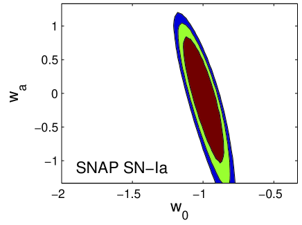
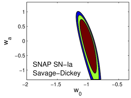
We begin by comparing our two methods of computing the Bayes factor, focussing on the SNAP mission supernova survey. The Bayes factor plots are shown in Figure 1. In the left panel we plot isocontours of Bayes factors in the $\hat{w}_{0}$–$\hat{w}_{a}$ plane inferred from the nested sampling method. The plot shows the generic structure expected of Bayes factor plots. In the central region, the simulated data are for models very close to $\Lambda$CDM, so that model gives a good fit and is further rewarded for its predictiveness, giving a positive Bayes factor which would support $\Lambda$CDM over the dark energy model. At the zero contour (the innermost one plotted) the models fare equally well, and then at greater distances the dark energy model becomes favoured. If the true parameters lie outside those contours, SNAP will be able to exclude $\Lambda$CDM at the probability corresponding to the contour level.

We see a strong degeneracy between the two parameters, meaning that supernova data are not good at constraining models in this particular parameter direction. This same degeneracy shows up in the usual Fisher matrix error projection method. Its precise direction depends on the redshift distribution of the supernovae.

Figure 2: This plot shows a parameter error forecast for the SNAP SN-Ia experiment, taking $\Lambda$CDM as the true model. The contour levels indicate 68% and 95%. While this figure uses the full likelihood, in this case a Gaussian approximation using the Fisher matrix gives essentially identical results.

In the right panel we plot the projected Bayes factor contours derived from the Savage–Dickey formula for the same experimental characteristics and priors assumed in the previous case. We see that this method gives generally good agreement with the nested sampling computation, indicating that our calculations are robust. Some slight differences are apparent, but this is expected as our version of the Savage–Dickey method employs a Gaussian approximation for the likelihood which may become poor at large distances from $\Lambda$CDM, with the Fisher matrix method underestimating the covariance matrix. For parameter estimation this is not a major concern, since deviations from the Gaussian approximation occur in the tail of the likelihood distribution, and quoted errors usually refer to the $68\%$ confidence intervals. However model selection calculations rely on good modelling well into the tails of the distribution.

Having verified that our methods give similar results, henceforth we will show results from the nested sampling method, since although it is computationally more intensive it does not assume a Gaussian likelihood.

Figure 3: Bayes’ factor forecasts for some future dark energy surveys. Contours are shown for $\log(B_{01})>0$, $-2.5$ and $-5$. An independent measurement of $\Omega_{{\rm m}}$ to $\pm 0.01$ is assumed. These plots show statistical uncertainties only, and several of these experiments are likely to be dominated by systematics.

4.2 Comparison with parameter error forecasting

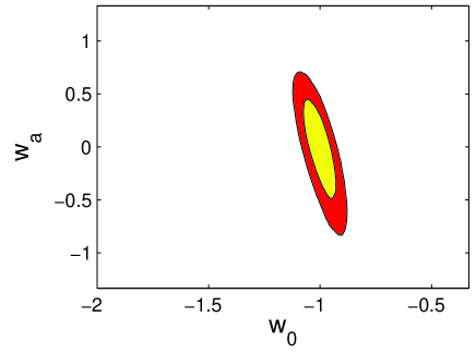
In this paper we are strongly advocating use of Bayes factor plots to quantify experimental capabilities, for the reasons enumerated in Section 2.2. It is useful to see explicitly what differences this gives as compared to the traditional parameter forecast approach, and so Figure 2 shows a plot of likelihood contours, obtained from a Markov chain Monte Carlo analysis of data simulated for the SNAP supernova survey, using precisely the same assumptions as Figure 1, and assuming that $\Lambda$CDM is the true model.

We see they share the same general shape, and that the same principal parameter degeneracy is picked out. Obviously the two plots are conceptually very different and so caution is needed in comparing. We see that the Bayes factor contours are significantly wider, indicating that model selection sets a more stringent condition for dark energy evolution to be supported by the data. Indeed, the 95% Fisher parameter contour lies within the $\ln B_{01}=0$ contour where model selection gives the models equal probability, hence by using the Fisher matrix plot we could rule out $\Lambda$CDM with data that actually favours it. It is fairly generic for that to be the case, indicating that 95% parameter estimation ‘results’ tend not to be robust under more sophisticated statistical analyses. This is a manifestation of Lindley’s ‘paradox’ as discussed by Trotta (2005) — that parameter values rejected under a frequentist test can nevertheless be favoured by Bayesian model selection.

4.3 Comparison of dark energy surveys

We now turn to a comparison of the six dark energy surveys described above. We stress once more that this comparison considers the statistical uncertainties alone, and several of these experiments are likely to be limited by systematics. The criteria that enable the systematics to be most effectively minimized are likely to be different from those giving experiments raw statistical power. Further we are working under the limitation of the particular $w_{0}$–$w_{a}$ parametrization; dark energy in reality could be different.

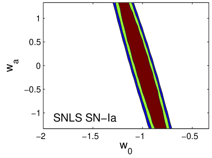
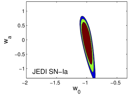
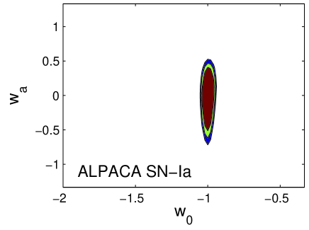
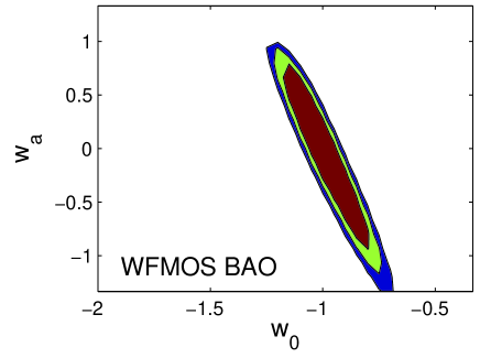
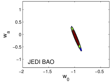
Figure 3 shows the six surveys, the upper four being supernova surveys and the lower two being the baryon acoustic oscillation surveys. The innermost contoured region is where the evidence of the $\Lambda$CDM model is greater than that of the evolving dark energy model ($\ln B_{01}>0$). The outer contours show $\ln B_{01}=-2.5$ and $-5$ so that the data provides strong evidence in favour of the evolving dark energy model. As with parameter estimation contours, the smaller the contours the more powerful the experiment is.

As expected, we see a range of constraining powers depending on the scale of the experiments. We also see that they broadly share the same principal degeneracy direction, with slight rotations visible from the different probing of redshift bins. The massive size of the expected ALPACA dataset gives it the smallest contour area amongst SN-Ia experiments, with its more limited redshift range making its degeneracy more vertical.

The baryon oscillation probes share almost the same principal degeneracy as the SNe-Ia; although they use the angular-diameter distance rather than the luminosity distance these two are related by the reciprocity relation and hence follow the same degeneracy shape if the uncertainties in each redshift bin follow the same shape. A probe which partly included the growth of structure, such as weak lensing, would be expected to have a somewhat different degeneracy; this has been shown using Fisher parameter contours for the SNAP lensing survey though the rotation is still smaller than one would like.

Note that the logarithms of the Bayes factors are additive, so if more than one of these surveys happen, or if there are two independent parts to a survey, then their Bayes factor plots can be added together to give a net Bayes factor plot.

In addition to plotting Bayes factor contours, one can further compress the information on how powerful an experiment is by computing the area within a particular contour level, to give a single ‘figure-of-merit’. Table LABEL:tab:areas summarizes these areas, expressed in coordinate units, for the six experiments, showing the area where $\ln B_{01}$ exceeds $-2.5$. Note that this corresponds to the parameter area in which an experiment cannot strongly exclude $\Lambda$CDM, and hence small numbers are better. For a more extensive discussion of figures-of-merit for optimization of dark energy surveys, in a parameter estimation rather than model selection framework, see Bassett (2005) and Bassett, Parkinson & Nichol (2005).

Table 1: Two experimental figures-of-merit: the areas in the $\hat{w}_{0}$–$\hat{w}_{a}$ plane where $\ln B_{01}$ exceeds $-2.5$, and the value of $\ln B_{01}$ at $\hat{w}_{0}=-1$ and $\hat{w}_{a}=0$. The former measures the region of parameter space where the experiment would not be able to exclude the $\Lambda$CDM model, while the latter measures the strength with which the experiment would support $\Lambda$CDM were it the true model. The $\ln B_{01}$ are additive between surveys and for independent probes of dark energy within the same survey.

Experiment	Area	$\ln B_{01}(-1,0)$
SNLS	0.51	3.7
SNAP	0.35	4.5
JEDI SN	0.19	5.0
ALPACA	0.08	6.1
WFMOS	0.26	4.8
JEDI BAO	0.04	6.0

4.4 Support for $\Lambda$CDM

We now consider the possibility of the experiments ruling out the dark energy model in favour of $\Lambda$CDM, rather than the opposite which we have focussed on thus far. Unlike parameter estimation methods, Bayesian model selection can offer positive support in favour of the simpler model. Because the simpler model is nested within the dark energy model, it can never fit the data better, but it can benefit from the volume effect of its smaller parameter space. All one needs to do is read off the Bayes factor for the case where the fiducial model is $\Lambda$CDM. Table LABEL:tab:areas shows $\ln B_{01}$ at $\hat{w}_{0}=-1$ and $\hat{w}_{a}=0$, i.e. when $\Lambda$CDM is the true model.

We find that this value is above 2.5 for all surveys, and above 5 for several of them. Thus many of the surveys are capable of accumulating strong evidence supporting $\Lambda$CDM over evolving dark energy. This can be seen as another figure of merit quantifying the power of experiments. Note again that the $\ln B_{01}$ are additive between surveys and for independent probes of dark energy within the same survey.

Note that the absolute value of this figure of merit is more sensitive to the prior ranges chosen for the dark energy parameters, which set the volume factor. However the relative comparison of surveys is again not affected by this.

Figure 4: Bayes’ factor forecasts for SNAP assuming different external knowledge of $\Omega_{\rm m}$. Contours are again shown for $\log(B_{01})>0$, $-2.5$ and $-5$. A Gaussian external constraint on $\Omega_{\rm m}$ is assumed, of width 0.03 (top panel) reflecting approximately the current level of uncertainty on it, and 0.003 (lower panel) reflecting an optimistic outcome.

4.5 Variation of assumptions

We end by examining the effect of varying some of the assumptions that went into the calculations, focussing on the SNAP supernova survey for definiteness. We do this in three ways, one by changing the presumed knowledge on $\Omega_{{\rm m}}$ that complements the dark energy survey, one by looking at an alternative prior in the dark energy model space, and finally by altering the assumed dispersion of supernova luminosities and allowing for a simple model of systematics.

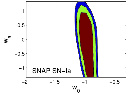
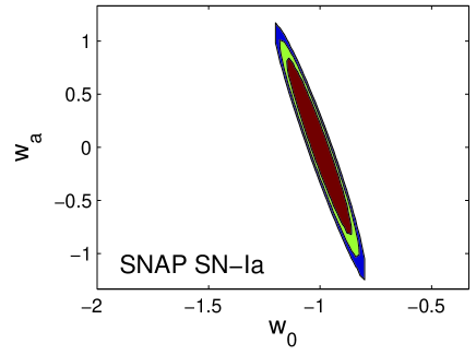
As mentioned before, the return on dark energy surveys is quite sensitive to the availability of external constraints to remove parameter degeneracies, particularly $\Omega_{{\rm m}}$ in the case of the supernovae. Figure 4 shows this effect for the SNAP supernova survey, with different constraints on $\Omega_{{\rm m}}$ to be compared with our standard assumption leading to the left panel of Figure 1. One sees a significant worsening of the Bayes factor contours in the case of weaker knowledge on $\Omega_{{\rm m}}$.

Altering the constraint on $\Omega_{{\rm m}}$ can have a different effect on different experiments. For instance, if it were more stringent, then the difference between SNLS and SNAP or JEDI would be greater — the requirement for a more sensitive experiment would be greater. Similarly the relative comparison is dependent on the nature of dark energy itself; if a parametrization more complex than $w_{0}$–$w_{a}$ proved necessary, it would be more important to make precise high-redshift observations (e.g. SNAP or JEDI versus ALPACA).

Figure 5: SNAP Bayes’ factor contours for the quintessence prior on $w_{0}$ and $w_{a}$. The lower left-hand region is cut off by the prior. The dashed contour shows the location of the $\ln B_{01}=-5$ contour for our full prior, as given in Figure 1.

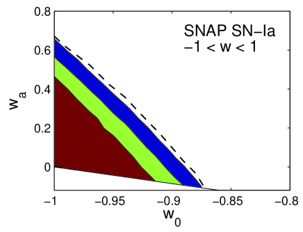
Figure 5 modifies our assumptions in a different way, this time altering the prior on the dark energy parameters. It assumes a prior appropriate to quintessence models, namely that $w\geq-1$ at all redshifts. The evidence integral for the dark energy model is then carried out over a narrower region in the dark energy parameters, giving a boost to the evidence of the dark energy model relative to $\Lambda$CDM. However the effect is small; the dashed line shows where the outer contour lay with our full dark energy prior and it has shrunk in only marginally.

Caldwell & Linder (2005) classified quintessence models into freezing and thawing models and delineated areas of the $w_{0}$–$w_{a}$ space where those models typically lie. According to Figure 5, freezing models can only be decisively distinguished from $\Lambda$CDM by the SNAP supernova survey if $\hat{w}_{0}\ga-0.9$, and thawing models if $\hat{w}_{0}\ga-0.87$.

We have also investigated how changing the prior ranges on the dark energy parameters alters the areas given in Table LABEL:tab:areas. In this case we narrowed the priors on $w_{0}$ and $w_{a}$ by a factor of two in each direction. In cases where the posterior still lies within the priors, this shifts the evidence by $\ln 4\simeq 1.4$ in favour of the dark energy model. Unsurprisingly, we find this reduces the areas within which $\Lambda$CDM cannot be excluded, typically by 10 to 20 per cent. Importantly, however, this change preserves the rankings of the experiments.

Figure 6: The main contours match the left panel of Figure 1, showing the SNAP supernova survey. Additionally, the dashed contour shows how the outer contour shifts under a simple modelling of systematics, and the dot-dashed contour shows how the outer contour would move if the magnitude error were smaller.

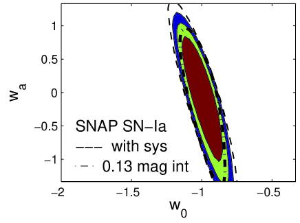
Finally, in Figure 6 we examine how the outer contour would shift if a smaller magnitude dispersion were achieved (we take $\delta_{m}=0.13$), and separately under a standard (but crude) modelling of possible systematics (see for example Kim et al. 2004). The systematics have been modelled as an increased redshift dependent uncertainty in magnitude of $(z/z_{\rm max})\delta m_{\rm sys}$ per redshift bin with $\delta m_{\rm sys}=0.02$ mag, and added in quadrature to the (intrinsic) statistical uncertainty. For SNAP, this type of systematic has quite a small effect. There can be other types of systematics in the data, but we do not try to model them here as the ability of different experiments to detect and (internally) resolve systematics would be different and a proper study of systematics and the required marginalization over them can only be done once the data arrive.

5 Conclusions

In this paper we have introduced the Bayes factor plot as a tool for assessing the power of upcoming experiments. It offers a full implementation of Bayesian model selection as a forecasting tool. As compared to the traditional parameter error forecasting technique, it offers a number of advantages enumerated in Section 2.2. Amongst those, perhaps the most important are that observational data is simulated at each point in the plane, rather than at a small number of fiducial models, and that the Bayes factor plot properly captures the experimental motivation as being one of model selection rather than parameter estimation.

As a specific example, we have used the Bayes factor plots to examine a number of proposed dark energy surveys, concentrating on their ability to distinguish between the $\Lambda$CDM model and a two-parameter dark energy model. Figure 3 indicates the region of parameter space outside which the true model has to lie, in order for the experiment to have sufficient statistical power to exclude $\Lambda$CDM using model selection statistics.

An important caveat is that our plots do not show the effects of systematics, which are likely to be the dominant uncertainty for many of the experiments. This drawback is shared by parameter error forecasts, and it is more or less the nature of systematic uncertainties that they cannot be usefully modelled in advance of actual observational data being obtained. In judging the true merit of an experimental proposal, it is therefore essential to judge how well structured it is for optimal removal of systematics, as well as looking at its raw statistical power.

While we have focussed on dark energy as a specific application, the concept of the Bayes factor plot has much broader applicability, and is suitable for deployment in a wide range of cosmological contexts.

Appendix A Marginalizing over simulated data

In the main body of the paper, we have plotted the Bayes factor as a function of the fiducial values of the dark energy parameters, assuming particular values for the other parameters in the fiducial model. In general, however, the Bayes factor is a function of all the fiducial model parameters, not just the ones of principal interest, though a practical problem is that we cannot easily plot the evidence ratio $B_{01}$ as a function of more than two variables $\hat{\theta}$.

One solution is marginalization over the parameters that we are not interested in, as one does in parameter estimation, assuming those parameters to lie within the range motivated by present data. As the fiducial parameters $\hat{\theta}$ belong to the definition of the data, we need to marginalize the evidences, $P(D|M)$, rather than the Bayes factors. Formally, the marginalization must take place in data space, so when we wish to integrate out a ‘nuisance’ parameter $\hat{\theta}_{\mu}$ which the data is a function of, we should take into account a transformation factor $\sqrt{\sum_{i}(\partial D_{i}/\partial\theta_{\mu})^{2}}$, evaluated at each $\hat{\theta}$ along the integral. However, provided the evidence varies only weakly over the relevant range of the fiducial models, or if our model depends (nearly) linearly on its parameters, then this function is a constant which cancels when computing the Bayes factor. In this case we can just average the evidences. This will also conserve the relation $B_{01}=1/B_{10}$.

In practice, the main determining factor in whether particular extra parameters are justified by the data is the true values of those parameters themselves, rather than values of the other parameters. Often, then, one can choose fixed values of the uninteresting parameters, presenting results on a slice through the fiducial parameter space. Indeed, this turns out to be the case for the dark energy surveys in this paper.

Appendix B Parameter error forecasting

In this paper we are advocating the use of Bayes factors to quantify the power of upcoming experiments, in place of parameter error forecasts. For comparison, we provide a brief overview of parameter error forecasting here, and discuss some of its features and limitations.

The idea is to simulate a sample of experimental data and then infer the parameter uncertainties using standard likelihood analysis. More specifically, assuming a model $M$ specified by a set of parameters $\theta=\{\theta_{\mu}\}$, a sample of data $D$ with the expected experimental errors is generated for a particular fiducial model with parameter values $\hat{\theta}$. Then a likelihood $P(D|\theta,M)$ is computed and the confidence intervals on the $\theta$ parameters are inferred by computing a posterior parameter probability distribution via Bayes’ rule,

$$P(\theta|D,M)=\frac{P(D|\theta,M)P(\theta|M)}{P(D|M)}.$$ (8)

As a result the parameter uncertainties depend both on the experimental characteristics and the choice of the fiducial model.

A simplified way of carrying out such an analysis is to use the Fisher matrix approximation. By construction the fiducial model parameter values $\hat{\theta}$ maximize the likelihood. Hence expanding $\ln{P(D|\theta,M)}$ to quadratic order in $\delta{\theta}\equiv\theta-\hat{\theta}$ one obtains (Bond 1995; Tegmark, Taylor & Heavens 1997)

$$P(D|\theta,M)\sim\exp{\left(-\frac{1}{2}\sum_{\mu\nu}F_{\mu\nu}\delta{\theta_{\mu}}\delta{\theta_{\nu}}\right)},$$ (9)

which is a Gaussian approximation to the likelihood with zero mean and with variance given by the inverse of the Fisher matrix $F_{\mu\nu}$, where

$$F_{\mu\nu}=\sum_{ij}C_{ij}^{-1}\frac{\partial D_{i}}{\partial\theta_{\mu}}\frac{\partial D_{j}}{\partial\theta_{\nu}}\,.$$ (10)

The sum is over all measurements and the partial derivatives are evaluated at the fiducial model parameter values $\hat{\theta}_{\mu}$. The matrix $C_{ij}$ is the data covariance matrix; for independent measurements (e.g. different supernovae) it simplifies to $\sigma^{2}(D_{i})\delta_{ij}$. The parameter errors are then given by the square root of the diagonal components of the covariance matrix, $\sigma(\theta_{\mu})=\sqrt{(F^{-1})_{\mu\mu}}$. It is evident from equation (10) that more accurate data, characterized by smaller uncertainty $\sigma(D)$, provide larger Fisher matrix components, hence smaller parameter errors. It can also be noticed that for a given experiment the parameters which are better constrained are those for which the partial derivatives are larger.

Since these derivatives are computed at the fiducial model, it is natural to expect that the size of the projected errors varies for different fiducial parameter values. These contours are usually plotted with the aim of drawing a conclusion based on the true model having different parameter values from those of the fiducial model. But the dependence on the choice of fiducial model means that there is no guarantee that the conclusions based on contours around e.g. the $\Lambda$CDM model can be used to rule that model out.

Figure 7: The marginalized $68\%$ and $95\%$ confidence contours in $\Omega_{{\rm m}}$–$w$ plane. The fiducial models are a $\Lambda$CDM with $w=-1$ and $\Omega_{{\rm m}}=0.3$ (solid line), a dark energy model with $w=-0.85$ and $\Omega_{{\rm m}}=0.35$ (dash-dot line), and a phantom model with $w=1.16$ and $\Omega_{{\rm m}}=0.26$ (dash line).

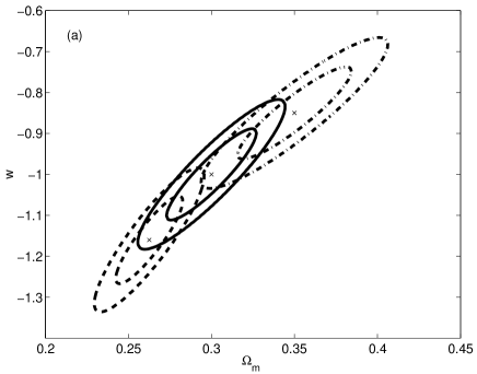
As an explicit example we compute the Fisher matrix errors of dark energy parameters from SN-Ia luminosity–distance measurements. We assume experimental characteristics from the proposed SNAP mission as discussed in Kim et al. (2004). We consider two different dark energy models, one parametrized by a constant equation of state parameter $w$, and a second by the two-parameter equation of state family of equation (3). We assume an independent measurement of $\Omega_{{\rm m}}$ with uncertainty $\pm 0.03$ to reduce parameter degeneracies, and compute the marginalized confidence contours around different fiducial models in $\Omega_{{\rm m}}$–$w$ and $w_{0}$–$w_{a}$ planes respectively.

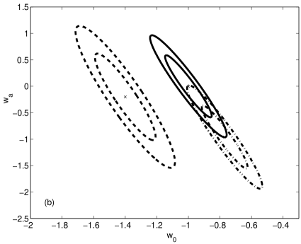
In Figure 7 we plot the $68\%$ and $95\%$ ellipses around three models: a $\Lambda$CDM model with $w=-1$ and $\Omega_{{\rm m}}=0.3$, a dark energy model with $w=-0.88$ and $\Omega_{{\rm m}}=0.35$, and a phantom model with $w=-1.16$ and $\Omega_{{\rm m}}=0.26$. The alignment of the strongest degeneracy line differs amongst the models. This is because the degeneracy in the $w-\Omega_{{\rm m}}$ plane is not a straight line, but rather a curve (see for instance Weller & Albrecht 2001). Notice also that the ellipses around the fiducial models have different sizes. As Fig. 7 shows, if the true model lies on say the 95% confidence limit of the $\Lambda$CDM data, one cannot necessarily presume that the $\Lambda$CDM model would lie on the 95% confidence limit of data simulated for the true model. It is possible to compute a contour indicating the locus of the fiducial models for which $\Lambda$CDM lies at their 95% confidence limit, and indeed such a locus is shown in Figure 1 of Kratochvil et al. (2004), but constructing it is a rather cumbersome procedure.

This drawback turns out to be less severe for dark energy models parametrized by equation (3). In Figure 8 we plot the $68\%$ and $95\%$ ellipses in the $w_{0}$–$w_{a}$ plane with $\Omega_{{\rm m}}=0.3$ around a $\Lambda$CDM model, a phantom model with $w_{0}=-0.8$ and $w_{a}=-1$ lying along the degeneracy line of the $\Lambda$CDM, and a constant phantom model with $w_{0}=-1.4$ and $w_{a}=-0.2$. The dependence on the fiducial model is still present, since the ellipses become larger as the fiducial model shifts orthogonal to the principal degeneracy direction towards more negative equation of state values. Fiducial models along the same degeneracy line whose $95\%$ contours include the $\Lambda$CDM model are within the $95\%$ ellipse of the $\Lambda$CDM as well.

Figure 8: Marginalized $68\%$ and $95\%$ contours in $w_{0}$–$w_{a}$ plane. The fiducial models are $\Lambda$CDM (solid line), a dark energy model with $w_{0}=-0.8$ and $w_{a}=-1$ (dash-dot line), and a phantom model with $w_{0}=-1.4$ and $w_{a}=-0.2$ (dash line). For all three models $\Omega_{{\rm m}}=0.3$.

References

- Aldering et al. (2004) Aldering G. et al. (SNAP collaboration), 2004, astro-ph/0405232
- Astier et al. (2006) Astier P. et al. (SNLS collaboration), 2006, A&A, 447, 31
- Bassett (2005) Bassett B. A., 2005, Phys. Rev. D, 71, 083517
- Bassett et al. (2004) Bassett B. A., Corasaniti P. S., Kunz M., 2004, ApJ, 617, L1
- Bassett et al. (2005) Bassett B. A., Parkinson D., Nichol R. C., 2005, ApJL, 626, L1
- Bond (1995) Bond J. R., 1995, Phys. Rev. Lett., 74, 4369
- Bond, Efstathiou & Tegmark (1997) Bond J. R., Efstathiou G., Tegmark M., 1997, MNRAS, 291, L33
- Caldwell and Linder (2005) Caldwell R. R., Linder E. V., 2005, Phys. Rev. Lett, 95, 141301
- Chevallier & Polarski (2001) Chevallier M., Polarski D., 2001, Int. J. Mod. Phys., D10, 213
- Corasaniti & Copeland (2003) Corasaniti P. S., Copeland E. J., 2003, Phys. Rev. D, 67, 063521
- Corasaniti et al. (2005) Corasaniti P. S., LoVerde M., Crotts A., Blake C., 2005, astro-ph/0511632
- Crotts et al. (2005) Crotts A. et al. (JEDI collaboration), 2005, astro-ph/0507043
- Dickey (1971) Dickey J. M., 1971, Ann. Math. Stat., 42, 204
- Efstathiou & Bond (1999) Efstathiou G., Bond J. R., 1999, MNRAS, 304, 75
- Gregory (2005) Gregory P., 2005, Bayesian Logical Data Analysis for the Physical Sciences, Cambridge University Press
- Jaffe (1996) Jaffe A., 1996, ApJ, 471, 24
- Jeffreys (1961) Jeffreys H., 1961, Theory of Probability, 3rd edition, Oxford University Press
- Jungman et al. (96) Jungman J., Kamionkowski M., Kosowsky A., Spergel D. N., 1996, Phys. Rev. D, 54, 1332
- Kass & Raftery (1995) Kass R. E., Raftery A. E., 1995, J. Amer. Stat. Assoc., 90, 773
- Kim et al. (2004) Kim A. G., Linder E. V., Miquel R., Mostek N., 2004, MNRAS, 347, 909
- Knox (1995) Knox L., 1995, Phys. Rev. D, 52, 4307
- Kratochvil et al. (2004) Kratochvil J., Linde A., Linder E. V., Shmakova M., 2004, JCAP, 0407, 1
- Linder (03) Linder E. V., 2003, Phys. Rev. Lett., 90, 091301
- LinHut (05) Linder E.V., Huterer D., 2005, Phys. Rev. D, 72, 043509
- MacKay (2003) MacKay D. J. C., 2003, Information theory, inference and learning algorithms, Cambridge University Press
- Marshall, Hobson & Slosar (2003) Marshall P. J., Hobson M. P., Slosar A., 2003, MNRAS, 346, 489
- Mukherjee et al. (2006) Mukherjee P., Parkinson D., Liddle A. R., 2006, ApJL, 638, L51
- Pogosian et al. (2005) Pogosian L., Corasaniti P. S., Stephan-Otto C., Crittenden R., Nichol R., 2005, Phys. Rev. D, 72, 103519
- Pritchet et al. (2004) Pritchet C. J. (SNLS Collaboration), 2004, astro-ph/0406242
- Saini, Weller & Bridle (2004) Saini T. D., Weller J., Bridle, S. L., 2004, MNRAS, 348, 603
- Seo & Eisenstein (2003) Seo H.-J., Eisenstein D. J., 2003, ApJ, 598, 720
- Skilling (2004) Skilling J., 2004, in Bayesian Inference and Maximum Entropy Methods in Science and Engineering, ed. R. Fischer et al., Amer. Inst. Phys., conf. proc., 735, 395 (available at http://www.inference.phy.cam.ac.uk/bayesys/).
- Tegmark et al. (2000) Tegmark M., Eisenstein D. J., Hu W., de Oliveira-Costa A., 2000, ApJ, 530, 133
- Tegmark et al. (1997) Tegmark M., Taylor A., Heavens A., 1997, MNRAS, 480, 22
- Trotta (2005) Trotta R., 2005, astro-ph/0504022.
- Verdinelli & Wasserman (1995) Verdinelli I, Wasserman L., 1995, J. Amer. Stat. Assoc., 90, 614
- Wang & Tegmark (2004) Wang Y., Tegmark M., 2004, Phys. Rev. Lett., 92, 241302
- Weller & Albrecht (2001) Weller J., Albrecht A., 2001, Phys. Rev. Lett., 86, 1939
- Zal (97) Zaldarriaga M., Spergel D. N., Seljak U., 1997, ApJ, 488, 1