The Mass Assembly History of Field Galaxies: Detection of an Evolving Mass Limit for Star Forming Galaxies

Abstract

We characterize the mass-dependent evolution in a large sample of more than 8,000 galaxies using spectroscopic redshifts drawn from the DEEP2 Galaxy Redshift Survey in the range $0.4<z<1.4$ and stellar masses calculated from $K$-band photometry obtained at Palomar Observatory. This sample spans more than 1.5 square degrees in four independent fields. Using restframe $(U-B)$ color and [OII] equivalent widths, we distinguish star-forming from passive populations in order to explore the nature of “downsizing”—a pattern in which the sites of active star formation shift from high mass galaxies at early times to lower mass systems at later epochs. Over the redshift range probed, we identify a mass limit, $M_{Q}$, above which star formation appears to be quenched. The physical mechanisms responsible for downsizing can thus be empirically quantified by charting the evolution in this threshold mass. We find that $M_{Q}$ decreases with time by a factor of $\approx$3 across the redshift range sampled according to $M_{Q}\propto(1+z)^{3.5}$. We demonstrate that this behavior is quite robust to the use of various indicators of star formation activity, including morphological type. To further constrain possible quenching mechanisms, we investigate how this downsizing signal depends on local galaxy environment using the projected 3^rd-nearest-neighbor statistic $D_{p,3}$ which is particularly well-suited for large spectroscopic samples. For the majority of galaxies in regions near the median density, there is no significant correlation between downsizing and environment. However, a trend is observed in the comparison between more extreme environments that are more than 3 times overdense or underdense relative to the median. Here, we find that downsizing is accelerated in overdense regions which host higher numbers of massive, early-type galaxies and fewer late-types as compared to the underdense regions. Our results significantly constrain recent suggestions for the origin of downsizing and indicate that the process for quenching star formation must, primarily, be internally driven. By quantifying both the time and density dependence of downsizing, our survey provides a valuable benchmark for galaxy models incorporating baryon physics.

1. Introduction

The redshift interval from $z\approx 1$ to $z=0$ accounts for roughly half of the age of the universe and provides a valuable baseline over which to study the final stages of galaxy assembly. From many surveys spanning this redshift range, it is now well-established that the global star formation rate (SFR) declines by an order of magnitude (e.g., Broadhurst et al., 1992; Lilly et al., 1996; Cowie et al., 1999; Flores et al., 1999; Wilson et al., 2002). An interesting characteristic of this evolution in SFR is the fact that sites of active star formation shift from including high mass galaxies at $z\gtrsim 1$ to only lower mass galaxies subsequently. This pattern of star formation, referred to by Cowie et al. (1996) as “downsizing,” seems contrary to the precepts of hierarchical structure formation and so understanding the physical processes that drive it is an important problem in galaxy formation.

The observational evidence for the downsizing of star formation activity is now quite extensive. The primary evidence comes from field surveys encompassing all classes of galaxies to $z\approx 1$ and beyond (Brinchmann & Ellis, 2000; Bell et al., 2005b; Bauer et al., 2005; Juneau et al., 2005; Faber et al., 2005; Borch et al., 2006). However, the trends are also seen in specific populations such as field spheroidals, both in their stellar mass functions (Fontana et al., 2004; Bundy et al., 2005) and in more precise fundamental plane studies (Treu et al., 2005; van der Wel et al., 2005) which track the evolving mass-to-light ratio as a function of dynamical mass. The latter studies find massive spheroidals completed the bulk of their star formation to within a few percent prior to $z\simeq$1, whereas lower mass ellipticals continue to grow by as much as 50% in terms of stellar mass after $z\sim 1$. Finally, detailed analyses of the spectra of nearby galaxies suggest similar trends (Heavens et al., 2004; Jimenez et al., 2005).

Downsizing is important to understand as it signifies the role that feedback plays in the mass-dependent evolution of galaxies. As a consequence, its physical origin has received much attention theoretically. Recent analytic work by Dekel & Birnboim (2004), for instance, suggests that the distinction between star-forming and passive systems can be understood via several characteristic mass thresholds governed by the physics of clustering, shock heating and various feedback processes. Some of these processes have been implemented in numerical and semi-analytic models, including mass-dependent star formation rates (Menci et al., 2005), regulation through feedback by supernovae (e.g., Cole et al., 2000; Benson et al., 2003; Nagashima & Yoshii, 2004) and active galactic nuclei (AGN) (e.g., Silk & Rees, 1998; Granato et al., 2004; Dekel & Birnboim, 2004; Hopkins et al., 2005; Croton et al., 2005; De Lucia et al., 2005; Scannapieco et al., 2005; Bower et al., 2005; Cattaneo et al., 2006). However, most models have, until now, primarily addressed the mass distinction between star-forming and quiescent galaxies as defined at the present epoch (e.g., Kauffmann et al., 2003b). Quantitative observational measures of the evolving mass dependence via higher redshift data have not been available.

This paper is concerned with undertaking a systematic study of how the mass-dependent evolution of galaxies progresses over a wide range of epochs. The goal is to quantify the patterns by which evolution proceeds as a basis for further modeling. Does downsizing result largely from the assembly history of massive early-type galaxies or is there a decline in the fraction of massive star-forming systems? In the quenching of star formation, what are the primary processes responsible and how are they related to the hierarchical framework of structure assembly as envisioned in the CDM paradigm? Does downsizing ultimately result from internal physical processes localized within galaxies such as star formation and AGN feedback, or is it caused by external effects related to the immediate environment, such as ram pressure stripping and encounters with nearby galaxies in groups and clusters?

In this paper, we combine the large spectroscopic sample contained in the DEEP2 Galaxy Redshift Survey (Davis et al., 2003) with stellar masses based on extensive near-infrared imaging conducted at Palomar Observatory to characterize the assembly history and evolution of galaxies since $z\approx 1.2$. Our primary goal is to quantify the downsizing signal in physical terms and test its environmental dependence so that it is possible to constrain the mechanisms responsible. A plan of the paper is as follows. Section $\S$2 presents the observations and characterizes the sample while $\S$3 describes our methods for measuring stellar masses, star formation activity and environmental density. We discuss how we estimate errors in the derived mass functions in $\S$4 and present our results in $\S$5. We discuss our interpretations of the results in $\S$6 and conclude in $\S$7. Where necessary, we assume a Chabrier IMF (Chabrier, 2003) and a standard cosmological model with $\Omega_{\rm M}=0.3$, $\Omega_{\Lambda}=0.7$, $H_{0}=100h$ km s^-1 Mpc^-1 and $h=0.7$.

2. Observations and Sample Description

Constraining the processes that govern downsizing requires a precise measure of the evolving stellar mass function of galaxies as a function of their physical state and environmental density. Achieving this ambitious goal requires multi-wavelength observations capable of revealing quantities such as the ongoing star formation rate in a large enough cosmic volume to reliably probe a range of environments. Among these requirements, two observational components are absolutely essential: a large spectroscopic survey and near-IR photometry.

Spectroscopic redshifts not only precisely locate galaxies in space and time, but enable the reliable determination of restframe quantities such as color and luminosity. This in turn allows for accurate comparisons to stellar population templates which provide stellar mass-to-light ratios ($M_{*}/L$) and the opportunity to convert from luminosity to stellar mass. As demonstrated in Bundy et al. (2005), relying on photometric redshifts (photo-$z$) decreases the typical precision of stellar mass estimates by more than a factor of three, with occasional catastrophic failures that lead to errors as large as an order of magnitude.

Spectroscopic redshifts are also crucial for determining accurate environmental densities (Cooper et al., 2005). Even with the most optimistic photometric redshift uncertainties of $\sigma_{z}=0.02$—COMBO-17 specifies $\sigma_{z}\approx 0.03$ (Wolf et al., 2003)—a comparison between photo-$z$ density measurements and the real-space density in simulated data sets gives a Spearman ranked correlation coefficient of only $\rho=0.4$ (where $\rho=1$ signifies perfect correlation, see Cooper et al., 2005). This uncertainty has the effect of smearing out the density signal in all but the lowest density environments in photo-$z$ samples. For the spectroscopic DEEP2 sample used in this paper, $\sigma_{z}=0.0001$ and $\rho=0.8$.

Spectroscopic observations also provide line diagnostics that can discriminate the star formation activity occurring in galaxies. Given the various timescales involved, it is useful to identify ongoing or recent star formation activity by considering various independent methods including restframe $(U-B)$ color, the equivalent width of [OII] $\lambda$3727, and galaxy morphology. Comparisons between the different indicators highlight specific differences between early- and late-type populations defined in different ways.

In addition to spectroscopy, the second essential ingredient in this paper is near-IR photometry. As suggested by Kauffmann & Charlot (1998) and first exploited by Brinchmann & Ellis (2000), near-infrared and especially $K$-band photometry traces the bulk of the established stellar populations and enables reliable stellar mass estimates for $z\lesssim 1.5$. With the addition of SED fitting from multi-band optical photometry, the uncertainty in such estimates can be reduced to factors of 2–3 based on $K$-band observations out to $z\approx 1.5$ (Brinchmann & Ellis, 2000). The importance of $K$-band observations is highlighted for galaxies with $z>0.75$, where the typical stellar mass uncertainty using the same technique applied to photometry with the z-band as the reddest filter would be worse by a factor of 3–4 (Bundy et al., in preparation). Uncertainties from optical mass estimates become even less secure as the redshift increases and increasingly bluer portions of the restframe SED are shifted into the reddest filter bands. Thus, the combined lack of $K$-band photometry and spectroscopic redshifts leads to stellar mass errors greater than factors of 5–10 with catastrophic failures off by nearly two orders of magnitude.

Because of these factors, the combination of the DEEP2 Galaxy Redshift Survey with panoramic IR imaging from Palomar Observatory represents the ideal (and perhaps only) data set for tracing the evolution of accurately measured stellar masses and various indicators of star formation activity across different environments to $z\approx 1.4$. We provide details on the specific components of this data set below.

2.1. DEEP2 Spectroscopy and Photometry

The DEEP2 Galaxy Redshift Survey (Davis et al., 2003) utilizes the DEIMOS spectrograph (Faber et al., 2003) on the Keck-II telescope and aims to measure $\sim$40,000 spectroscopic redshifts with $z\lesssim 1.5$ for galaxies with $R_{AB}\leq 24.1$. The survey samples four widely-separated regions, covering a total area of 3.5 square degrees. Targeting of the spectroscopic sample was based on $BRI$ photometry obtained at the Canada–France–Hawaii Telescope (CFHT) with the 12K$\times$8K mosaic camera (Cuillandre et al., 2001). Catalogs selected in the $R$-band were constructed using the imcat photometric package (Kaiser et al., 1995) and reach a limiting magnitude of $R_{AB}\sim 25.5$ (Coil et al., 2004). The photometric calibration was computed with respect to Sloan Digital Sky Survey (SDSS) observations which overlap a portion of the CFHT sample. The observed colors, used to estimate the inferred restframe $(U-B)$ colors in this paper, were measured using apertures defined by the object size in the $R$-band image. Further details on the CFHT photometry can be found in Coil et al. (2004).

Sources were targeted for DEIMOS spectroscopy based on several criteria. As determined by magnitude, color, and size, objects in the photometric catalog were assigned a probability, $P_{gal}$, for being a galaxy. Redshift targets were required to have $P_{gal}>20\%$ with magnitudes in the range, $18.5\leq R_{AB}\leq 24.1$ (see Willmer et al., 2005). In DEEP2 Fields 2–4, targets were also color-selected in $(B-R)$ vs. $(R-I)$ color space to lie predominantly at redshifts greater than 0.7. Details on the color cuts will be presented in Faber et al. (in preparation). These selection criteria successfully recover 97% of the $R_{AB}\leq 24.1$ population at $z>0.75$ with only $\sim$10% contamination from lower redshift galaxies (Davis et al., 2005). The redshift survey in these three fields is now complete, providing a total of 21592 successful redshifts over 3 square degrees. The last field, the Extended Groth Strip (EGS) covers 0.5 square degrees and is currently 75% complete with a total of 9501 galaxies in the range $0<z<1.5$. The selection of targets in EGS is magnitude-limited, providing a valuable sample for verifying the success of the color selection used in Fields 2–4. The sampling rate of galaxies satisfying the target criteria is $\sim$60% and DEEP2 galaxies from all 4 fields are included in this paper.

DEEP2 redshifts were determined by comparing various templates to observed spectra as well as fitting specific spectral features. This process is interactive and will be described in Newman et al. (in preparation). Spectroscopic redshifts are used in this paper only when two or more features have been identified in a given spectrum (giving “zquality” values $\geq 3$, Faber et al., 2005). The fraction of objects for which this process fails to give a reliable redshift is roughly 30% and is dominated by faint blue galaxies, the majority of which are beyond $z\sim 1.4$ where the [OII] $\lambda$3727 feature is redshifted beyond the DEEP2 spectral wavelength range (Willmer et al., 2005). More details on the redshift success rate are provided in Willmer et al. (2005), and Coil et al. (2004) further discuss the survey strategy and spectroscopic observations.

2.2. Palomar Near-IR Imaging

Motivated largely by this study, we have conducted an extensive panoramic imaging survey of all four DEEP2 fields with the Wide Field Infrared Camera (WIRC, Wilson et al., 2003) on the 5m Hale Telescope at Palomar Observatory. We describe the salient points of this survey here and will provide further observational details in a later article (Bundy et al., in preparation).

The Palomar survey commenced in fall 2002 and was completed after 65 nights of observing in October 2005. Using contiguously spaced pointings (each with a camera field-of-view of 8$\farcm$6$\times$8$\farcm$6) tiled in a 3$\times$5 pattern, we mapped the central third of Fields 2–4 to a median 80% completeness depth greater than $K_{AB}=21.5$, with 5 pointings deeper than $K_{AB}=22.5$. The imaging in Fields 2–4 accounts for 0.9 square degrees or 55% of the Palomar K_s-band survey.

The remainder of the data was taken in the EGS where the K_s-band data covers 0.7 square degrees, but to various depths. The EGS was considered the highest priority field in view of the many ancillary observations—including HST, Spitzer, and X-ray imaging—obtained there. As the orientation of the WIRC camera is fixed on the sky and the EGS traces a $\sim$45 degree strip 16′ wide, to fully cover the spectroscopic field in the E–W direction requires rows of three WIRC pointings. The N–S direction requires about 12 different positions, so, in total, 35 WIRC pointings were used to map the EGS in the K_s-band. The deepest observations were obtained along the center of the strip where there is complete overlap between WIRC and the spectroscopically-surveyed area. In these regions, the typical depth is greater than $K_{AB}=22.5$. The rest of the southern half of the EGS reaches $K_{AB}=22.3$, while that for the northern half is complete to $K_{AB}=21.7$. Additional Palomar $J$-band observations were obtained for most of the central strip of the EGS and for Fields 3 and 4. These provide $J$-band photometry for roughly half of the K_s-band sample and are useful in improving photometric redshifts.

Individual K_s-band exposures at a given pointing were taken with an integration time of 2 minutes using coadditions of either 4 $\times$ 30 seconds in average temperature conditions, 3 frames $\times$ 40 seconds in cooler conditions, or 6 frames $\times$ 20 seconds in warm conditions. The exposures were dithered at 27 positions in a non-repeating, pseudo-random $\approx$7″pattern and combined into 54-minute mosaics using a double-pass reduction pipeline developed specifically for WIRC. At a given pointing, individual mosaics were often obtained on different nights and so may vary in terms of seeing, sky background levels and transparency. Most K_s-band pointings consist of more than two independently-combined mosaics with the deepest pointings comprising as many as 6 independent mosaics. Mosaic coaddition was performed using an algorithm that optimizes the depth of the final image by applying weights based on the seeing, background, and transparency of the subframes. The final seeing FWHM in the K_s-band images ranges from 0$\farcs$8 to 1$\farcs$2, and is typically 1$\farcs$0. Photometric calibration was carried out by referencing standard stars during photometric conditions and astrometric registration was performed with respect to DEEP2 astrometry (see Coil et al., 2004) using bright stars from the CFHT $R$-selected catalog. More details on the survey strategy and image processing are presented in Bundy et al. (in preparation).

After masking out the low signal-to-noise perimeter of the final K_s-band images, we used SExtractor (Bertin & Arnouts, 1996) to detect and measure the K_s-band sources. As an estimate of the total K_s-band magnitudes, which are used to derive the luminosity and stellar mass of individual galaxies (see $\S$3.1), we use the MAG_AUTO output from SExtractor. We do not adjust this Kron-like magnitude to account for missing light in extended sources, which introduces two slight biases in our total magnitudes. First, the average difference between the MAG_AUTO values of a given galaxy and its corresponding magnitude measured in a 4″ diameter aperture is $\approx$0.03 mag fainter at the highest redshifts compared to the lowest redshifts in the sample. This effect leads to a systematic underestimate of 0.01 dex in stellar masses at high-$z$ compared to low-$z$. In addition, MAG_AUTO systematically underestimates the total magnitude of blue galaxies (defined by restframe $U-B$ color, see 3.2) in the lowest redshift interval as compared to red galaxies. The magnitude of this effect, which likely results from the more extended nature of typical blue galaxies, is also $\approx$0.03 mag but is not significant in the middle or high redshift intervals. Considering these systematic effects contribute less than 0.01 dex to the final stellar mass estimates, we do not explicitly correct for them.

In addition to total magnitudes, we also use SExtractor to measure aperture photometry in diameters of 2″, 3″, 4″, and 5″. To determine the corresponding magnitudes of K_s-band sources in the CFHT $BRI$ and Palomar $J$-band images, we applied the IDL photometry procedure, APER, to these data, placing apertures with the same set of diameters at sky positions determined by the K_s-band detections (all magnitudes were corrected to airmass = 1). This method was adopted with the aim of producing a $K$-selected catalog—about 25% of the K_s-band sources do not have optical counterparts in the CFHT imcat catalog. Magnitudes measured with APER are consistent with SExtractor aperture magnitudes, and experimentation with color-color diagrams and photometric redshifts demonstrated that the 2″ diameter colors exhibited the least scatter. We therefore use the 2″ aperture colors for fitting template spectral energy distributions (SEDs) to constrain stellar mass estimates, as well as to estimate photo-$z$’s for sources beyond the DEEP2 spectroscopic limit.

Photometric errors and the K_s-band detection limit of each image were estimated by randomly inserting fake sources of known magnitude into each K_s-band image and recovering them with the same detection parameters used for real objects. The inserted objects were given Gaussian profiles with a FWHM of 1$\farcs$3 to approximate the shape of slightly extended, distant galaxies. We define the detection limit as the magnitude at which more than 80% of the simulated sources are detected by SExtractor. Robust photometric errors based on simulations involving thousands of fake sources were also determined for the $BRI$ and $J$-band data. These errors are used to determine the uncertainty of the stellar masses and in the determination of photometric redshifts, where required.

2.3. The Primary Sample

Given the various ingredients necessary for the data set, it is helpful to construct separate samples based on the differing completeness limits for the $R$-limited spectroscopic sample and the $K$-limited Palomar catalog.

We will define the primary sample as that comprising galaxies with DEEP2 spectroscopic redshifts that are also detected in the Palomar K_s-band imaging. Redshift counterparts were found by cross-referencing the K_s-band catalog with the DEEP2 redshift catalog. A conservative tolerance of 1$\farcs$1 in the difference between the K_s-band and DEEP2 positions was used to select matches, although the offset for most sources was less than 0$\farcs$5. The relatively low surface density of both catalogs assures that the number of spurious associations is less than 1–2 percent. The fraction of DEEP2 redshifts detected in the K_s-band varies from $\approx$65% for K_s-band depths near $K_{AB}=21.7$ to $\approx$90% for $K_{AB}=22.7$. After removing the redshift survey boundaries to allow for unbiased density estimates (see $\S$3.3), Fields 2, 3, and 4 host 953, 1168, and 1704 sample galaxies respectively, all with secure spectroscopic redshifts in the range $0.75<z<1.4$. The fourth field, the EGS, contains 4770 galaxies with redshifts in the range $0.2<z<1.4$.

In the analysis that follows, we divide this sample into three broad redshift intervals. The first, $0.4<z<0.7$, contains 943 galaxies, drawn entirely from the EGS while the second ($0.75<z<1.0$, 2210 galaxies) and third ($1.0<z<1.4$, 1430 galaxies) draw from all four fields (see Table 1). Although the entire spectroscopic sample was selected to have $R_{AB}\leq 24.1$, the limiting K_s-band magnitude was chosen separately for each redshift interval. Because the Palomar K_s-band survey covers different areas to different depths, the area and volume of a given subsample depend on the K_s-band limit that is applied. This is advantageous and allows us to choose limits for each redshift bin that maintain adequate statistics and stellar mass completeness while producing subsamples that probe similar cosmological volumes—an important consideration for making environmental comparisons in a consistent fashion. In the three redshift bins, we select galaxies with secured K_s-band detections brighter than 21.8, 22.0, and 22.2 (AB), respectively. In the standard cosmology we have adopted with $h=0.7$, the areas sampled with these limits result in comoving volumes of 0.5, 1.4, and 2.3 in units of $10^{6}$ Mpc³.

Table 1Sample statistics

	Primary Spec-$z$, $R_{AB}\leq 24.1$		Photo-$z$ Supplemented, $R_{AB}\leq 25.1$
Sample	Number		Number	$f_{{\rm spec\mbox{-}}z}$	$f_{{\rm ANN}z}$	$f_{\rm BPZ}$
EGS Field
Full sample	2669		8540	36%	51%	13%
$0.4<z<0.7$	943		3026	36%	62%	2%
$0.75<z<1.0$	1003		2801	42%	46%	12%
$1.0<z<1.4$	723		2713	29%	43%	28%
DEEP2 Fields 2–4
Full sample	1914		10156	21%	68%	11%
$0.4<z<0.7$	—		4264	2%	97%	1%
$0.75<z<1.0$	1207		2865	42%	48%	10%
$1.0<z<1.4$	707		3027	27%	47%	26%

Note. — The listed values reflect cropping the DEEP2 survey borders to allow for accurate environmental density measurements (see $\S$3.3) and, for the three redshift intervals, K_s-band magnitude cuts of 21.8, 22.0, and 22.2 (AB).

2.4. The Photo-$z$ Supplemented Sample

As mentioned previously, photometric redshifts are insufficient for accurate density measurements (Cooper et al., 2005), do not offer [OII]-based SFR estimates, and significantly decrease the precision of stellar mass (Bundy et al., 2005) and restframe color estimates. However, photometric redshifts do offer the opportunity to augment the primary sample and extend it to fainter magnitudes, providing a way to test for the effects of incompleteness in the primary spectroscopic sample because of the various magnitude limits and selection procedures. With this goal in mind, we constructed a comparison sample using the optical+near-IR photometry described above to estimate both photometric redshifts and stellar masses. We discuss the importance of this comparison in interpreting our results in section $\S$4.2.

Photometric redshifts were derived in two ways. First, because the DEEP2 multi-slit masks do not target every available galaxy, there is a substantial number of objects that satisfy the photometric criterion of $R_{AB}\leq 24.1$ without spectroscopic redshifts. These are ideal for neural network photo-$z$ estimates because of the availability of a large spectroscopic training set. For these galaxies, we use ANN$z$ (Collister & Lahav, 2004) to measure photo-$z$’s, training the network with the EGS spectroscopic sample so that the ANN$z$ results cover the full range, $0.2<z<1.4$, without being subject to biases from any color selection. Based on comparisons to the spectroscopic samples in Fields 2–4, the ANN$z$ results are in excellent agreement with $\Delta z/(1+z)\approx 0.07$.

While the $R_{AB}\leq 24.1$ ANN$z$ photo-$z$ results present a complete sample, they do not contain fainter galaxies because no spectroscopic sample is available to train them. We therefore define a second sample of galaxies with $24.1<R_{AB}\leq 25.1$ and 3$\sigma$ detections in the $BIK$ bands. For these we use the BPZ photo-$z$ package (Benítez, 2000) and 2$\farcs$0 diameter aperture photometry, including $J$-band where available. We first optimize BPZ by comparing to spectroscopic samples. These tests reveal a systematic offset in the BPZ results that likely arises from the assumed HDF-North prior (Benítez, 2000). We fit a linear relation to this offset and remove it from all subsequent BPZ estimates. This improves the spectroscopic comparison to $\Delta z/(1+z)\approx 0.17$. For sources with $R_{AB}\leq 24.1$, we find good agreement between the ANN$z$ and BPZ results, although the BPZ estimates exhibit a larger degree of scatter.

Using the ANN$z$ and BPZ results, we construct photo-$z$ supplemented samples in each redshift bin with an $R$-band limit of $R_{AB}\leq 25.1$. The first bin, with $0.4<z<0.7$, contains 7290 galaxies; 16% have spectroscopic redshifts (available in the EGS only), 83% have ANN$z$ photo-$z$’s, and only 1% have BPZ photo-$z$’s. The second bin, with $0.75<z<1.0$, contains 5666 galaxies; 42% have spectroscopic redshifts, 48% have ANN$z$ photo-$z$’s, and 10% have BPZ photo-$z$’s. The third bin, with $0.75<z<1.0$, contains 5740 galaxies; 28% have spectroscopic redshifts, 45% have ANN$z$ photo-$z$’s, and 27% have BPZ photo-$z$’s. The sample statistics are summarized in Table 1.

3. Determining Physical Properties

The goal of this paper is to derive key physical quantities that can be used to describe the stellar mass, evolutionary state, and environmental density of galaxies, and to use these measures to understand the physical processes that drive the broad patterns observed. In this section we discuss our methods for reliably determining these key variables by making use of the unique combination of spectroscopy and near-IR imaging offered by the DEEP2/Palomar survey described above. The uncertainties discussed below refer to the primary sample. Our full error analysis is described in $\S$4.1.

3.1. Stellar Masses Estimates

$K$-band luminosities alone provide stellar mass estimates that are uncertain by factors of 5–7 (Brinchmann, 1999). However, for samples of known spectroscopic redshift, using optical-infrared color information can constrain the stellar population and $M_{*}/L$ ratio so as to reduce this uncertainty to $\simeq$0.2 dex. In this paper, we employ such a technique using the method described in Bundy et al. (2005) and discussed further in Bundy et al. (in preparation). We use a code that is Bayesian in nature and based on the precepts described in Kauffmann et al. (2003a) and Brinchmann & Ellis (2000).

Briefly, the code uses $BRIK$ colors (measured using 2$\farcs$0 diameter aperture photometry matched to the $K$-band detections) and spectroscopic redshifts to compare the observed SED of a sample galaxy to a grid of 13440 synthetic SEDs (from Bruzual & Charlot, 2003) spanning a range of star formation histories (parametrized as an exponential), ages (restricted to be less than the age of the universe at the observed redshift), metallicities, and dust content. The choice of models and population synthesis code employed can introduce systematic uncertainties. For example, Maraston et al. (2006) show that popular recipes such as those in Bruzual & Charlot (2003) do not accurately chart the evolution of Thermally-Pulsing Asymptotic Giant Branch stars. For young template models (with ages less than 2 Gyr), the Maraston models predict stellar masses that can be lower by as much as $\sim$60%. We note this potential source of error, but do not explicitly correct for it in estimating stellar masses here.

Once the grid of models has been defined, the K_s-band $M_{*}/L_{K}$, minimum $\chi^{2}$, and the probability that each model accurately describes a given galaxy is calculated at each grid point. The corresponding stellar mass is then determined by scaling $M_{*}/L_{K}$ ratios to the K_s-band luminosity based on the total K_s-band magnitude and redshift of the observed galaxy. The probabilities are then summed (marginalized) across the grid and binned by model stellar mass, yielding a stellar mass probability distribution for each sample galaxy. We use the median of the distribution as the best estimate.

The stellar mass measured in this way is robust to degeneracies in the model, such as those between age and metallicity. Although these degeneracies can produce bimodal probability distributions, even in these cases, the typical width of the distribution gives uncertainties from the model fitting alone of 0.1–0.2 dex. For about 2–3% of the SED fits, the minimum $\chi^{2}$ values are significantly greater than 1.0. For these more poorly-constrained objects, we add an additional 0.2 dex in quadrature to the final mass uncertainty. Although in principle, the best fitting model also provides estimates of the age, metallicity, star formation history, and dust content of a sample galaxy, these quantities are much more affected by degeneracies and are poorly constrained compared to the stellar mass.

We also note that real galaxies are likely to have more complex star formation histories than the simple stellar populations assumed here. However, we do not attempt to fit the observed SEDs with more complicated models, including those with multiple components and bursts, because our photometric observations do not provide sufficient constraints. More complex models are particularly relevant to galaxies with recent bursts of star formation which can hide underlying stellar mass. Several authors have investigated this effect. Studying the most extreme possibilities, Shapley et al. (2005), for example, find that the stellar mass of blue galaxies with recent starbursts could be underestimated by a factor of 5. More typical values are probably much less, and Tran et al. (2004) estimate the fraction of post starbursts identified as E+A galaxies in the range $0.3<z<1$ to be a few percent (although see Yan et al., 2005), so the effect of starbursts in our sample is likely to be small.

Photometric errors enter the stellar mass analysis by determining how well the template SEDs can be constrained by the data. Larger photometric uncertainties “smear out” the portion of the model grid that fits an observed galaxy with high probability. This is reflected in a wider stellar mass probability distribution. Additional uncertainties in the K_s-band luminosity (from errors in the observed total K_s-band magnitude) lead to final stellar mass estimates that are typically good to 0.2–0.3 dex. The largest systematic source of error comes from the assumed IMF, in this case that proposed by Chabrier (2003). The stellar masses we derive using this IMF can be converted to Salpeter by adding $\sim$0.25 dex, although we note this offset represents an average with a scatter across the models in our grid of $\sim$0.06 dex.

3.2. Indicators of Star Formation Activity

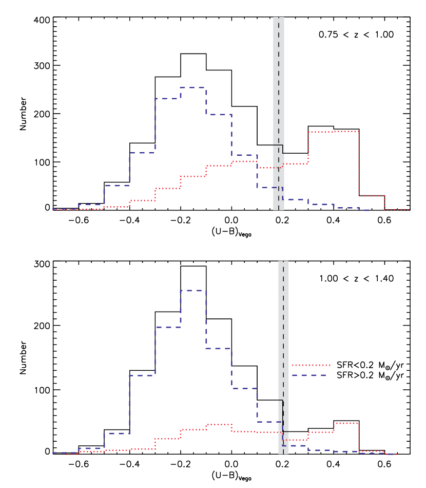
Figure 1.— The restframe $(U-B)$ color distribution in the middle and high redshift bins. Overplotted are the distributions of galaxies whose star formation rate as derived from the [OII] equivalent width is greater than 0.2 M_⊙/yr (blue dashed line) and less than 0.2 M_⊙/yr (red dotted line). The $(U-B)$ bimodality discriminant and its 1$\sigma$ range is indicated by the vertical dashed line and grey shading.

In this paper, we adopt two independent approaches for identifying those galaxies that are undergoing, or have recently experienced, active star formation. The first is the restframe $(U-B)$ color, estimated with the same methods as in Willmer et al. (2005) and based on the imcat photometry measured for the CFHT $BRI$ data. The $k$-corrections, which translate observed $BRI$ colors into restframe $(U-B)$ values, are determined by comparison to a set of 43 nearby galaxy SEDs from Kinney et al. (1996). Second-order polynomials were used to estimate $(U-B)$ and $k$-corrections as a function of observed color. Appendix A in Willmer et al. (2005) provides more details on this technique.

The $(U-B)$ color distribution exhibits a clear bimodality that is used to divide our sample into “Blue” (late-type) and “Red” (early-type) subsamples using the same luminosity-dependent color cut employed by van Dokkum et al. (2000):

$$U-B=-0.032(M_{B}+21.52)+0.454-0.25$$ (1)

This formula, defined in the Vega magnitude system, divides the sample well at all redshifts (see Figure 1), and so we do not apply a correction for potential rest-frame evolution with redshift (Willmer et al., 2005). We note that the proportion of red galaxies at high-$z$ in Figure 1 is in part suppressed by the $R$-band selection limit of $R_{AB}=24.1$ (selection effects are discussed in detail in $\S$4.2).

For galaxies with $z>0.75$, the [OII] 3727 Å emission line falls within the spectroscopic range probed by the DEEP2 Survey and this can be used to provide a second, independent estimate of the SFR. For these galaxies, we measure the intensity of the [OII] emission line by fitting a double gaussian—with the wavelength ratio constrained to that of the [OII] doublet—using a non-linear least squares minimization. We measure a robust estimate of the continuum by taking the biweight of the spectra in two wavelength windows each 80 Å long and separated from the emission line by 20 Å. We consider only spectra where the equivalent width of the feature is detected with greater than 3$\sigma$ confidence.

Because the DEEP2 spectra are not flux calibrated, we use the following formula from Guzman et al. (1997) to estimate the [OII] SFR:

$${\rm SFR(M_{\odot}~{}yr^{-1})}\approx 10^{-11.6-0.4(M_{B}-M_{B\odot})}{\rm EW_{[OII]}}$$ (2)

This relation utilizes the restframe $M_{B}$ estimated in the same way as the $(U-B)$ colors (see Willmer et al., 2005) and provides an approximate value for the SFR without correcting for metallicity effects, which can introduce random and systematic errors of at least 0.3–0.5 dex in the SFR derived from ${\rm L_{[OII]}}$ (Kewley et al., 2004). In addition, Equation 2 was optimized for a sample of compact emission line galaxies (see Guzman et al., 1997) which likely differs in the amount of extinction and typical [OII]/H$\alpha$ ratio compared to the sample here, yielding SFR estimates that could be systematically off by a factor of $\sim$3. Moreover, recent work by Papovich et al. (2005) demonstrates that SFR’s based on re-radiated IR radiation can be orders of magnitude larger than optical/UV estimates, and studies of the AGN population in DEEP2 indicate that [OII] emission is often associated with AGN, further biasing [OII]-based SFR estimates (Yan et al., 2005). Future efforts, especially those utilizing the multi-wavelength data set in the EGS, will be useful in refining the SFR estimates. In the present paper, we accept the limitations of Equation 2 for determining absolute SFR’s, noting that our primary requirement is not a precision estimate of the SFR for each galaxy but only the broad division of the field population into active and quiescent subsets.

In support of this last point, Figure 1 compares the $(U-B)$ and [OII] star formation indicators directly in the two higher redshift bins where both diagnostics are available. The solid histogram traces the full $(U-B)$ distribution with the vertical dashed line (and shading) indicating the median and 1$\sigma$ range of the color bimodality discriminant (the range results from the dependence on $M_{B}$ in Equation 1). Using the independent diagnostic of the [OII] equivalent width, we can similarly divide the population into high (blue dashed histogram) and low (red dotted histogram) star-forming populations using a cut of ${\rm SFR_{[OII]}}=0.2$ M_⊙ yr^-1, which is the median SFR of galaxies with $0.75<z<1.0$. Figure 1 clearly shows the effectiveness of the $(U-B)$ color cut in distinguishing the populations in both cases. The fraction of red galaxies in the high ${\rm SFR_{[OII]}}$ population is less than 8% in the middle redshift bin and less than 17% in the high-$z$ bin. The fact that a non-zero fraction of blue galaxies is made up of the low ${\rm SFR_{[OII]}}$ population is likely indicative of the 1–2 Gyr timescale required for galaxies to join the red sequence and suggests that even minor episodes of star formation can lead to blue restframe colors (Gebhardt et al., 2003). In addition, the median value of the measured [OII] SFR increases in the high-$z$ bin. This means that galaxies satisfying the ${\rm SFR_{[OII]}}=0.2$ M_⊙ yr^-1 cut at high redshift are more vigorously forming stars, and therefore bluer.

Further details on the evolving SFR will be presented in Noeske et al. (in preparation). We also note that the $(U-B)$ and [OII] star formation indicators are consistent with the star formation histories recovered by the SED template fitting procedure used to refine stellar mass estimates and described in $\S$3.1. This agreement is expected because the restframe color and SED fitting are both determined by the observed colors. Such consistency demonstrates that the measured physical properties that we use to divide the galaxy population are also reflected in the best-fit SED templates that determine stellar mass (see $\S$3.1).

3.3. Environmental Density

Figure 2.— The distribution in the relative overdensity in log units as measured across the sample by the 3^rd-nearest-neighbor statistic as implemented by Cooper et al. (2005). The vertical dotted lines at $\pm$0.5 dex divide the distribution into low, middle, and high density regimes (see text for details).

Charting galaxy evolution over a range of environments represents a key step forward that can only be achieved through large spectroscopic redshift surveys such as in the DEEP2 survey. Cooper et al. (2005) rigorously investigate the question of how to provide precise environmental density estimates in the context of redshift surveys at $z\sim 1$. That work clearly shows, via comparisons to simulated samples, that large samples with photo-$z$’s are very poorly suited to providing accurate density measures in all but the most underdense environments.

Specifically, Cooper et al. (2005) find that for environmental studies at high-$z$, the projected $n^{th}$-nearest-neighbor distance, $D_{p,n}$, offers the highest accuracy over the greatest range of environments. This measure is the field counterpart to projected density estimates first applied to studies of cluster environments (e.g., Dressler, 1980). The statistic is defined within a velocity window ($\Delta v=\pm 1000$ km s^-1) used to exclude contaminating foreground and background galaxies. It is therefore particularly robust to redshift space distortions in high density environments without suffering in accuracy in underdense environments. In addition, the effect of survey boundaries on $D_{p,n}$ is easily understood and mitigated by excluding a small strip around survey edges.

In this paper, we utilize the projected $3^{rd}$-nearest-neighbor distance, $D_{p,3}$, excluding galaxies closer than 1 $h^{-1}$ Mpc ($\sim$3′) from a survey boundary. The choice of $n=3$ does not significantly affect $D_{p,n}$ which has a weak dependence on $n$ in both high and low density environments for $n\leq 5$ (Cooper et al., 2005). The effects of survey target selection must be carefully considered because they can introduce biases as a function of redshift. Cooper et al. (2005) find that the sampling rate and selection function in the DEEP2 survey equally probes all environments at $z\sim 1$ in a uniform fashion. Although the DEEP2 survey secures redshifts for roughly 50% of galaxies at $z\sim 1$, its sparse selection algorithm does not introduce a significant environment-dependent bias. However, the absolute value of $D_{p,3}$ will increasingly underestimate the true density with increasing redshift as the sampling rate declines. To handle this effect, we first convert $D_{p,3}$ into a projected surface density, $\Sigma_{3}$, using $\Sigma_{3}=3/(\pi D_{p,3}^{2})$. We then calculate the relative overdensity at the location of each galaxy by dividing the observed value of $\Sigma_{3}$ by the median surface density calculated in bins of $\Delta z=0.04$. The relative overdensity is thus insensitive to the DEEP2 sampling rate, providing a reliable statistic that can be compared across the full redshift range of the sample (Cooper et al., 2005). We note that a small bias in this statistic may be introduced by the fact that DEEP2 preferentially selects blue galaxies as the redshift increases. Tests indicate this effect is smaller than the typical density uncertainty (a factor of $\sim$3) and is not likely to be important given the coarse density bins we use to divide the sample. Further details are provided in Cooper et al. (2006).

The distribution of the relative overdensity for our primary sample is plotted in Figure 2. In the analysis that follows, we consider two ways of dividing the sample by environmental density. In the first, we separate galaxies according to whether they lie in regions above or below the median density (corresponding to a measured overdensity of zero in Figure 2). This is the simplest criterion but does mean the bulk of the signal is coming from regions which are not too dissimilar in their environs. In the second approach, we divide the density sample into three bins as indicated by the vertical dotted lines in Figure 2. The thresholds of 0.5 dex, or 0.77$\sigma$, above and below the median density were chosen to select the extreme ends of the density distribution where the field sample begins to probe group and void-like environments that are 3–100 times more or less dense than average. The conclusions presented in $\S$5 are not sensitive to the precise location of these three thresholds.

4. Constructing the Galaxy Stellar Mass Function

The DEEP2/Palomar survey presents a unique data set for constraining the galaxy stellar mass function at $z\sim 1$. Previous efforts have so far relied on smaller and more limited samples, often without spectroscopic redshifts. Only via the combination of size, spectroscopic completeness, and depth, does the current sample enable us to study the evolving relationships between stellar mass, star formation activity, and local environment in a statistically robust way. Our primary tool in this effort is charting the galaxy stellar mass function of various populations.

Deriving the stellar mass function in a magnitude limited survey requires corrections for the fact that faint galaxies are not detected throughout the entire survey volume. The $V_{max}$ formalism (Schmidt, 1968) is the simplest technique for handling this problem but does not account for density inhomogeneities that can bias the shape of the derived mass function. While other techniques address this problem (for a review, see Willmer, 1997), they face different challenges such as determining the total normalization. For sufficiently large samples over significant cosmological volumes, density inhomogeneities cancel out and the $V_{max}$ method produces reliable results. Considering this and the fact that we wish to use our data set to explicitly test for the effects of density inhomogeneities, we adopt the $V_{max}$ approach, which offers a simple way to account for both the $R$ and K_s-band limits of our sample. For each galaxy $i$ in the redshift interval $j$, the value of $V^{i}_{max}$ is given by the minimum redshift at which the galaxy would leave the sample, becoming too faint for either the $R$ or K_s-band limit. Formally, we define

$$V^{i}_{max}=d\Omega_{j}\int_{z_{low}}^{z_{high}}\frac{dV}{dz}dz$$ (3)

where $d\Omega_{j}$ is the solid angle subtended by the sample defined by the limiting K_s-band magnitude, $K^{j}_{lim}$, for the redshift interval $j$, and $dV/dz$ is the comoving volume element. The redshift limits of the integral are:

$$z_{high}={\rm min}(z^{j}_{max},z^{j}_{K_{lim}},z_{R_{lim}})$$ (4)

$$z_{low}=z^{j}_{min}$$ (5)

where the redshift interval, $j$, is defined by $[z^{j}_{min},z^{j}_{max}]$, $z^{j}_{K_{lim}}$ refers to the redshift at which the galaxy would still be detected below the K_s-band limit for that particular redshift interval, and $z_{R_{lim}}$ is the redshift at which the galaxy would no longer satisfy the $R$-band limit of $R_{AB}\leq 24.1$. We use the SED template fits found by the stellar mass estimator to calculate $z^{j}_{K_{lim}}$ and $z_{R_{lim}}$, thereby accounting for the $k$-corrections necessary to compute accurate $V_{max}$ values (no evolutionary correction is applied).

In constructing the $V_{max}$ mass functions, we also weight the spectroscopic sample to account for incompleteness resulting from the DEEP2 color selection and redshift success rate. We closely follow the method described in Willmer et al. (2005), but add an extra dimension to the reference data cube which stores the number of objects with a given K_s-band magnitude. Thus, for each galaxy $i$ we count the number of objects from the photometric catalog sharing the same bin in the $(B-R)$/$(R-I)$/$R_{AB}$/K_s-band parameter space as well as the fraction of these with attempted and successful redshifts. As mentioned in $\S$2.1, $\approx$30% of attempted DEEP2 redshifts are unsuccessful, mostly because of faint, blue galaxies beyond the redshift limit accessible to DEEP2 spectroscopy (Willmer et al., 2005). Failed redshifts for red galaxies are more likely to be within the accessible redshift range but simply lacking in strong, identifiable features. We therefore use the “optimal” weighting model (Willmer et al., 2005), which accounts for the redshift success rate by assuming that failed redshifts of red galaxies (defined by the $(U-B)$ color bimodality) follow the same distribution as successful ones, while blue galaxies with failed redshifts lie beyond the redshift limit ($z\approx 1.5$) of the sample. The final weights are then based on the probability that a successful redshift would be obtained for a given galaxy. They also account for the selection function applied to the EGS sample to balance the fraction of redshifts above and below $z\approx 0.7$. With the weight, $\chi_{i}$, calculated in this way, we determine the differential galaxy stellar mass function:

$$\Phi(M_{*})dM_{*}=\sum_{i}\frac{\chi_{i}}{V^{i}_{max}}dM_{*}$$ (6)

4.1. Uncertainties and Cosmic Variance

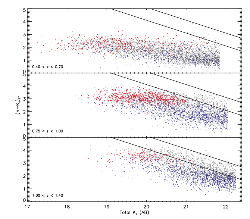
Figure 3.— Apparent color-magnitude diagrams used to illustrate sample completeness. The plots show the distribution of $(R-K_{s})$ vs $K_{s}$ for the primary spectroscopic redshift sample with $R_{AB}\leq 24.1$ (solid, color circles) compared to the $R_{AB}\leq 25.1$ sample, which has been supplemented with photometric redshifts (small black dots). The spectroscopic sample is colored according to location in the bimodal restframe $(U-B)$ distribution as described in the text. The $R_{AB}=24.1$ and $R_{AB}=25.1$ magnitude limits are indicated by the solid diagonal lines.

Figure 4.— Completeness of the mass distribution in the primary spectroscopic sample taking into account the $R$-band and K_s-band magnitude cuts. The left-hand panels show the completeness resulting from the $R_{AB}\leq 24.1$ limit as derived from comparisons within the photo-$z$ supplemented sample. Vertical dotted lines indicate the mass of the faintest galaxy that could be detected at the high-$z$ end of each redshift interval, while vertical dashed lines correspond to galaxies at the low-$z$ end. The right-hand panels, also drawn from the $R_{AB}\leq 25.1$ sample, show the effect of the K_s-band limit on the mass completeness. Vertical dotted and dashed lines indicate model galaxy limits, as in the left panels. The more conservative dotted lines are adopted as the mass limits of the paper.

To estimate the uncertainty in our mass distribution we must account for several sources of random error and model their combined effect through Monte Carlo simulations. Different error budgets are calculated for the primary spectroscopic and photo-$z$ supplemented samples via 1000 realizations of our data set in which we randomized the expected errors. In both samples we model uncertainties in $V_{max}$ arising from photometric errors, and simulate the error on the stellar mass estimates, which, as described in $\S$3.1, is typically 0.2 dex and is encoded in the stellar mass probability distribution of each galaxy.

For the primary spectroscopic sample, errors on the rest-frame $(U-B)$ colors are estimated by noting the photometric errors for a given galaxy. We do not model the uncertainty in the [OII] SFR because unaccounted systematic errors are likely to be greater than the random uncertainty of measurements of the [OII] equivalent width. We stress again that these diagnostics are only used to separate the bimodal distribution into active and quiescent components.

For the photo-$z$ supplemented sample, we model redshift uncertainties using $\Delta z/(1+z)=0.07$ for the $R_{AB}\leq 24.1$ ANN$z$ subsample and $\Delta z/(1+z)=0.18$ for the $R_{AB}\leq 25.1$ BPZ subsample. The BPZ uncertainty is slightly higher than measured in the comparison to the spectroscopic sample because we expect a poorer precision of BPZ on objects with $R_{AB}>24.1$. These redshift uncertainties affect the distribution of objects in our redshift bins as well as the Monte Carlo realizations of stellar mass estimates in the photo-$z$ sample. The final uncertainty at each data point in the stellar mass functions from both the spectroscopic and photo-$z$ supplemented samples is estimated conservatively as the sum, in quadrature, of the 1$\sigma$ Monte Carlo errors and the Poisson errors.

We now turn to cosmic variance. Because our sample is drawn from four independent fields, it is possible to estimate the effects of cosmic variance by comparing the results from different fields in each of our three redshift bins: $0.4<z<0.7$, $0.75<z<1.0$, and $1.0<z<1.4$. For the spectroscopic sample with $z>0.75$, we can compare the EGS to the sum of Fields 2, 3, and 4, yielding two subsamples with roughly equal numbers of galaxies. We compare the total and color-dependent stellar mass functions of these two subsamples and divide the median of the differences measured at all data points by $\sqrt{2}$ to estimate the cosmic variance. Unfortunately, galaxies with $z<0.75$ come only from the EGS. The cosmic variance estimate here is derived by performing the same calculation on three subsets of the EGS sample and dividing it by $\sqrt{3}$. Of course, cosmic variance on the scale of the EGS itself is not included in this estimate. For the three redshift intervals, this method provides average 1$\sigma$ systematic cosmic variance uncertainties of 29%, 12%, and 26%.

In addition to these rough estimates, we have checked that the observed density distribution is not affected by cosmic variance. Based on the density-dependent mass functions from different fields, there is no evidence of a single structure or overdensity in one of the fields that would bias our results. We also note that the type-dependent mass functions are, to first order, affected by cosmic variance in the same way as the total mass functions. Thus, while absolute comparisons between different redshift intervals must account for cosmic variance errors, comparisons using the relative or fractional abundance of a given population are less susceptible to this uncertainty. For example, comparisons between different fields of the abundance of blue galaxies at $z\sim 0.5$ with masses near $M_{*}=10^{10.8}$M_⊙ (see $\S$5) suggest that the absolute measurement is uncertain at the $\sim$40% level, while the relative measurement made with respect to the total abundance of galaxies is uncertain only at the $\sim$15% level. For red galaxies in this same bin, the standard deviation for the relative fraction is 10%, but increases to 25% for the measurement of their absolute abundance.

4.2. Completeness and Selection Effects

We now turn to the important question of the redshift-dependent completeness of the stellar mass functions in our sample. Incompleteness resulting from the DEEP2 selection technique is corrected for by applying weights to galaxies within the spectroscopic sample, as described in $\S$4. The $R$ and K_s-band limits of this sample also introduce incompleteness effects, however, that cannot be corrected through weighting. Instead, we adopt two approaches to determine how the incompleteness from our magnitude limits affects the derived mass functions.

First, we consider the likelihood of observing model galaxies of known mass and color based on the $R$ and K_s-band magnitude limits of the primary spectroscopic sample. We follow previous work (e.g., Fontana et al., 2003) and track the stellar mass of a template galaxy with a reasonable maximum $M_{*}/L$ ratio determined by models with solar metallicity, no dust, and a burst of star formation beginning at $z_{form}=5$ that lasts for 0.5 Gyr and is then truncated. We set the luminosity according to the $R$ and K_s-band limiting magnitudes. The maximum stellar masses of these model galaxies provide estimates of our completeness limits. We consider two realizations. In the first, the model is placed at the low-$z$ edge of each redshift interval where the intrinsically faintest galaxies would be detected (such galaxies have high $V_{max}$ weights). In the second, more conservative limit, the model is placed at the high-$z$ edge of the interval, representing the faintest systems that could be detected across the entire redshift bin. The results indicate that the K_s-band limit ensures completeness above $3\times 10^{10}$M_⊙ at all redshifts, while the $R$-band limit primarily affects our high-$z$ sample below $10^{11}$M_⊙. We discuss these limits in detail below.

Our second approach is to measure the effects of incompleteness directly by comparing our primary spectroscopic sample with $R_{AB}\leq 24.1$ to the fainter sample with $R_{AB}\leq 25.1$, supplemented by photometric redshifts. This approach is particularly useful for investigating the way in which the $R$-band limit introduces a bias against red galaxies, especially at $z\gtrsim 1$. This bias could mimic the effect of downsizing by suppressing the fraction of red galaxies at $z\gtrsim 1$. The behavior of model galaxies (described above) as well as the comparison to a fainter sample both yield consistent estimates for the sample completeness which we will show does not compromise our results.

Figure 3 compares the distribution in 2$\farcs$0 diameter $(R-K_{s})$ vs total $K_{s}$ color-magnitude space of the primary spectroscopic sample with $R_{AB}\leq 24.1$ (solid color circles) to that for the fainter $R_{AB}\leq 25.1$ sample (small black dots) supplemented with photometric redshifts. As expected, in the low redshift bin, the majority of the $R_{AB}\leq 25.1$ sample is contained within the spectroscopic limit of $R_{AB}=24.1$ (although the photo-$z$ sample includes many more galaxies with $R_{AB}\leq 24.1$ that were not selected for spectroscopy). At high redshift, however, the primary sample is clearly incomplete, with a substantial number of galaxies having $R_{AB}>24.1$. While the full range of $(R-K_{s})$ colors is included in the primary sample, a color bias is introduced because the reddest galaxies are no longer detected at $K_{AB}\gtrsim 20$.

To demonstrate how this color bias affects the mass completeness of the sample, the left-hand panels in Figure 4 chart the stellar mass completeness of the photo-$z$ supplemented sample limited to $R_{AB}\leq 24.1$ as compared to the full sample with $R_{AB}\leq 25.1$. With increasing redshift, the fraction of galaxies satisfying $R_{AB}\leq 24.1$ decreases. This results in a loss of detected galaxies below a given mass which corresponds closely to the conservative limits based on model galaxies placed at the high-$z$ edge of each redshift interval, as described above and indicated by the dotted vertical lines in Figure 4. However, because of the $V_{max}$ weighting, our analysis is actually more complete than the figure suggests. A more appropriate completeness limit is indicated by the vertical dashed line, which corresponds to model galaxies at the low-$z$ edge of each redshift interval where the faintest galaxies are still detected.

Figure 4 indicates that for galaxies with $z<1$, the $R$-band limit has only a small effect on the spectroscopic sample. Galaxies with $R_{AB}\leq 24.1$ constitute the vast majority of the total distribution in the first two redshift bins, with a minimum completeness of $\approx$80% in the middle redshift bin. The $R$-band limit has a greater effect in the high-$z$ bin, where the $R_{AB}\leq 24.1$ distribution accounts for just over $\approx$60% of the $R_{AB}\leq 25.1$ sample over most of the mass range. We note that the $R$-band limit affects mostly red galaxies which we will show dominate at higher masses. For this reason, the completeness function resulting the $R$-band limit rises again at lower masses. In section $\S$5, we correct for the $R$-band incompleteness and show that it does not affect our conclusions.

The right-hand panels of Figure 4 illustrate the effect of the K_s-band limit on the mass completeness of the spectroscopic sample. Using our deepest Palomar observations, we construct stellar mass distributions from the photo-$z$ supplemented sample with $R_{AB}\leq 25.1$. Again, for each redshift interval, we compare the mass distribution of a subsample with a K_s-band limit equal to 0.5 magnitudes fainter than the limit imposed on the spectroscopic sample at that redshift, $K^{j}_{lim}$. As in the left-hand panels of Figure 4, the resulting completeness function yields an estimate of the K_s-band mass completeness limit that is consistent with the high-$z$ and low-$z$ model galaxy masses described above. For the analysis to follow, we conservatively adopt the high-$z$ model limits indicated by the dotted lines, although we acknowledge that heavily obscured galaxies may still be missed above these limits. For each redshift bin, these limits correspond to 10.1, 10.2, and 10.4 in units of $\log$ M_⊙. We note that for the middle and high redshift bins in which the $R$-band limit affects the sample, the K_s-band completeness limit occurs at lower masses, justifying our method for studying the $R$ and K_s-band limits separately.

5. Results

5.1. The Total Stellar Mass Function

The total galaxy stellar mass functions in three redshift intervals are plotted in Figure 5. Results for both the spectroscopic, $R_{AB}\leq 24.1$ sample (solid circles, dark shading) and $R_{AB}\leq 25.1$, photo-$z$ supplemented sample (open diamonds, light shading) are presented. The width of the shaded curves corresponds to the final 1$\sigma$ errors using the Monte Carlo techniques discussed earlier. For the $R_{AB}\leq 24.1$ sample, the lowest redshift interval draws only from the EGS, leading to a larger cosmic variance uncertainty as indicated by the isolated error bar in the upper right portion of the plot. The $R_{AB}\leq 24.1$ mass functions in the two higher redshift bins, as well as the $R_{AB}\leq 25.1$ sample in all bins, utilize data from all four DEEP2 survey fields. The close agreement between the spectroscopic and photo-$z$ supplemented total mass functions indicates that the weighting applied to compensate for the DEEP2 spectroscopic selection function in the $R_{AB}\leq 24.1$ sample is successful at recovering a complete, magnitude-limited sample. The vertical dotted lines represent estimates of the mass completeness originating from the K_s-band magnitude limit (see $\S$4.2). The solid curve plotted for all three redshift intervals is the Schechter fit to the $R_{AB}\leq 25.1$ mass function at $z\sim 0.55$, and can be used to gauge evolution within our sample.

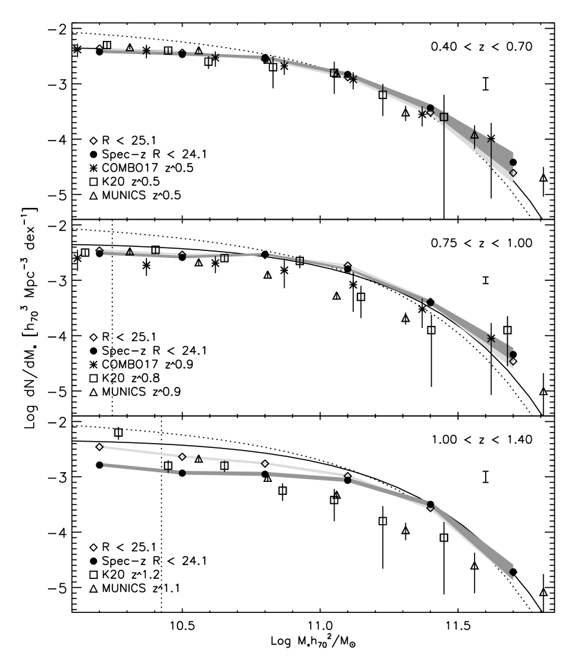
Figure 5.— Total stellar mass functions in three redshift bins. Shading indicates the width of 1$\sigma$ error bars. The mass function for all galaxies in the primary spectroscopic sample is designated by solid circles with dark shading. That for the deeper, $R_{AB}\leq 25.1$ sample, supplemented by photo-$z$’s, is indicated by open diamonds and light gray shading. Results from the COMBO17 (Borch et al., 2006), K20 (Fontana et al., 2004), and MUNICS (Drory et al., 2004) surveys are also plotted. The dotted curve is the Schechter fit to the local mass function from Cole et al. (2001). The solid curve is a Schechter fit to the $R_{AB}\leq 25.1$ results in the first redshift bin. Vertical dotted lines show estimates for the mass completeness limit resulting from the K_s-band magnitude limits—in the highest redshift interval incompleteness resulting from the $R$-band limit becomes important, as demonstrated by the difference between the spectroscopic and photo-$z$ supplemented mass functions. The isolated error bar in the upper right-hand portion of each plot indicates the estimated average uncertainty due to cosmic variance.

As discussed in $\S$4.2, the mass functions of the primary sample presented in Figure 5 are affected by incompleteness because of the $R_{AB}=24.1$ spectroscopic limit. The degree of incompleteness is apparent in the comparison between the total mass functions of the spectroscopic and $R_{AB}\leq 25.1$ samples. As expected from Figure 4, the first two redshift bins are hardly affected by $R$-band incompleteness. However, the $R_{AB}=24.1$ limit is clearly important in the high redshift bin where the comoving number density in the photo-$z$ sample is larger by a factor of $\approx$2 (0.3 dex) for $M_{*}<10^{10.8}$M_⊙.

Figure 5 also plots results from several previous studies, all of which have been normalized to $h=0.7$ and adjusted for comparison to the Chabrier IMF used here. The dotted curve is the Schechter fit to the local stellar mass function as determined by Cole et al. (2001). Results from the K20 (Fontana et al., 2004), MUNICS (Drory et al., 2004), and COMBO17 (Borch et al., 2006) surveys are also plotted. The K20 survey (Cimatti et al., 2002) has good spectroscopic coverage (92%) but is shallower than the data presented here and covers only 52 square arcminutes or 0.01 square degrees. The MUNICS survey (Drory et al., 2001) covers roughly one square degree, but only reaches $K\sim 19.5$ (Vega) and is composed of 90% photometric redshifts. The COMBO17 results utilize carefully calibrated photo-$z$’s (Wolf et al., 2004) and represent an area of 0.8 square degrees, but infrared photometry was not available. Instead, Borch et al. (2006) scale their stellar mass estimates to the magnitude measured in a narrow filter (21 nm wide) at 816Å. This restricts the redshift range where masses can be estimated to $z<1$.

The stellar mass functions from previous work as well as the new results presented here are in good agreement in the first redshift bin in Figure 5. It is interesting to note that all of the results plotted find a higher abundance of massive galaxies ($M_{*}\gtrsim 5\times 10^{11}$M_⊙) and a lower abundance of less massive galaxies ($M_{*}\lesssim 6\times 10^{10}$M_⊙) compared to the local mass functions of Cole et al. (2001), although a slight excess above the Schechter fit is also seen at the highest masses in local samples (e.g., Cole et al., 2001). We do not plot the local mass function from Bell et al. (2003) because it is in good agreement with Cole et al. (2001). Borch et al. (2006) argue that the higher number of massive galaxies in their study may be caused by photo-$z$ errors, but we find similar results in our spectroscopic sample. This discrepancy may reflect systematic differences in the way stellar masses are estimated, and highlights potential difficulties in comparing high-$z$ work to local studies.

Our mass function at $z\sim 0.9$ shows little evolution compared to the lower redshift interval. In fact, for $M_{*}\gtrsim 10^{11}$M_⊙, we find slightly higher number densities at $z\sim 0.9$, but this is likely due to cosmic variance. Our results are consistent with the COMBO17 mass functions but are higher than the K20 and MUNICS mass functions, a difference that seems to increase in the highest redshift bin. Here we find only a slight decrease in the numbers of galaxies with $M_{*}\gtrsim 3\times 10^{11}$M_⊙, an effect that is consistent with no evolution, given the uncertainties from cosmic variance. The photo-$z$ supplemented mass function at $z\sim 1.2$ reveals a more significant decline, however, with respect to our low-$z$ bin in the number density of lower mass galaxies (with $M_{*}\lesssim 3\times 10^{11}$M_⊙). This hints at the notion that the mass assembly history of all galaxies may proceeds in a top-down fashion, lending support to recent claims of so-called “mass assembly downsizing” (e.g., Cimatti et al., 2006). While intriguing, we postpone a detailed analysis of this effect to a future paper, choosing instead to focus on downsizing in the context of star formation activity.

Table 2Schechter Fit Parameters

	$\phi^{*}$	$\log h_{70}M^{*}$	$\alpha$
Redshift	($h_{70}^{3}$ Mpc-3 dex-1)	(M⊙)
Primary Spec-$z$, $R_{AB}\leq 24.1$
$0.4<z<0.7$	$0.0027\pm 0.0004$	$10.94\pm 0.08$	$-0.81\pm 0.2$
$0.75<z<1.0$	$0.0031\pm 0.0010$	$10.87\pm 0.10$	$-0.59\pm 0.4$
$1.0<z<1.4$	$0.0012\pm 0.0008$	$10.97\pm 0.25$	$-0.51\pm 0.5$
Photo-$z$ Supplemented, $R_{AB}\leq 25.1$
$0.4<z<0.7$	$0.0025\pm 0.0007$	$10.93\pm 0.11$	$-0.95\pm 0.1$
$0.75<z<1.0$	$0.0031\pm 0.0014$	$10.87\pm 0.10$	$-0.51\pm 0.4$
$1.0<z<1.4$	$0.0015\pm 0.0004$	$11.01\pm 0.07$	$-0.93\pm 0.1$

Note. — Quoted uncertainties were estimated based on field-to-field comparisons.

In Table 2, we list the parameters of Schechter fits to the $R_{AB}\leq 24.1$ and photo-$z$ supplemented, $R_{AB}\leq 25.1$ mass functions plotted in Figure 5. By integrating the photo-$z$ Schechter fits we obtain estimates for the global stellar mass density in units of $\log$ M_⊙ $h_{70}$ Mpc^-3 of $\log\rho_{*}=8.31\pm 0.07$ at $z\sim 0.55$, $\log\rho_{*}=8.30\pm 0.1$ at $z\sim 0.9$, and $\log\rho_{*}=8.15\pm 0.1$ at $z\sim 1.2$, where the uncertainties come from cosmic variance estimates based on field-to-field comparisons. These results are in good agreement with previous measurements of $\rho_{*}$ (Dickinson et al., 2003; Rudnick et al., 2003; Drory et al., 2005).

5.2. The Mass Functions of Blue and Red Galaxies

We now partition the total mass functions presented in Figure 5 into active and quiescent populations according to the bimodality observed in the restframe $(U-B)$ color. The results are illustrated in Figure 6, which for reference also plots the total mass functions from Figure 5. As before, the vertical dotted lines indicate the onset of incompleteness resulting from the K_s-band limit, and the solid curve is a Schechter fit to the photo-$z$ supplemented total mass function in the first redshift interval.

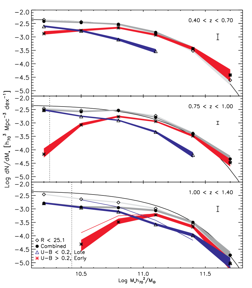
Figure 6.— Mass functions in three redshift bins partitioned by rest-frame $(U-B)$ color as described in the text. Shading indicates the width of 1$\sigma$ error bars. The mass function for all galaxies in the primary spectroscopic sample is designated by solid circles. That for the deeper, $R_{AB}\leq 25.1$ sample, supplemented by photo-z’s, is indicated by open diamonds. Vertical dotted lines show estimates for mass incompleteness resulting from the K_s-band magnitude limit. In the high-redshift bin (bottom panel), thin red and blue lines trace the expected increase in the red and blue populations if the spectroscopic limit of $R_{AB}=24.1$ were extended by one magnitude. The isolated error bar in the upper right-hand portion of each plot indicates the estimated systematic uncertainty due to cosmic variance. The solid curve in each panel shows the Schechter fit to the photo-$z$ supplemented mass function in the first redshift interval.

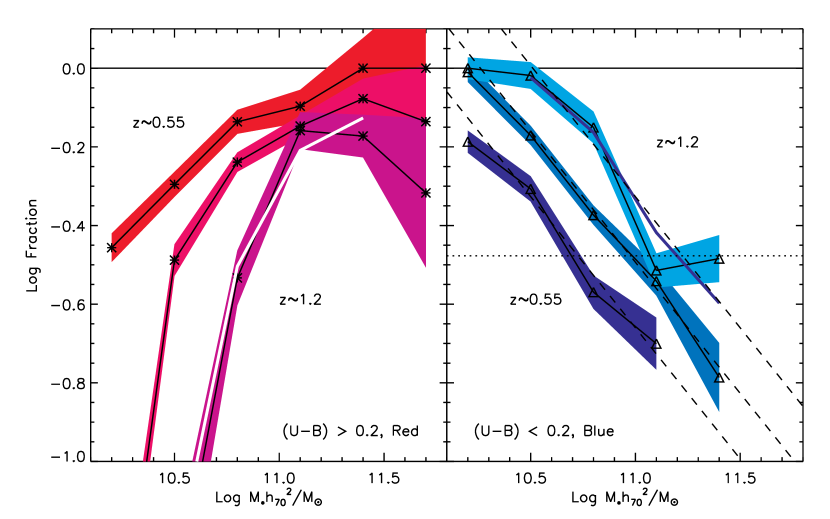
Figure 7.— Log fractional contribution of the red and blue populations to the total stellar mass function at various redshifts. The relative contribution of red galaxies (left plot) increases with cosmic time, while that for blue galaxies decreases (right plot). The expected high-$z$ fraction of red and blue types after correcting for $R$-band completeness (as in Figure 6) is shown by a thin white line for the red population and a thin blue line for the blue population. The corrected fractions from the $R_{AB}\leq 25.1$ sample are entirely consistent with those observed in the primary $R_{AB}\leq 24.1$ spectroscopic sample. Dashed lines in the right-hand panel show approximate fits to the declining fraction of blue galaxies. $M_{Q}$ is defined by where these lines cross the dotted horizontal line, which marks a fractional abundance of 1/3 the total value. (see $\S$5.4).

As discussed above, the $R\leq 24.1$ limit introduces incompleteness in the high redshift bin. To mitigate this effect we derive a color-dependent completeness correction for the high-$z$ bin based on the photo-$z$ supplemented $R\leq 25.1$ sample. Inferring the restframe $(U-B)$ color for this sample is difficult because of photometric redshift uncertainties. Instead, we adopt the simpler approach of applying a color cut in observed $(R-K)$, which, as shown in Figure 3, maps well onto the restframe $(U-B)$ color for the high-$z$ spectroscopic sample. We tune the $(R-K)$ cut so that the resulting color-dependent mass functions of the $R_{AB}\leq 25.1$ sample match the spectroscopic ($R_{AB}\leq 24.1$) mass functions above $M_{*}=10^{11.3}$M_⊙ where the spectroscopic sample is complete. This yields a value of $(R-K_{s})_{2^{\prime\prime}}=3.37$, consistent with the $(U-B)$ bimodality apparent in the color-magnitude diagram shown in Figure 1.

Using this observed $(R-K)$ color cut for the high-$z$ bin only, we show the color-dependent mass functions for the $R_{AB}\leq 25.1$ sample in Figure 6 as thin white and blue lines. While these curves suffer from their own uncertainties, such as photo-$z$ errors and a less precise measure of color, they are useful for illustrating the nature of the $R$-band incompleteness in the spectroscopic sample. It is important to note that while the deeper sample yields higher mass functions for both the red and blue populations below $M_{*}\approx 10^{11.1}$M_⊙, the relative contribution of each one to the total mass function is similar to what is observed in the spectroscopic sample. This is shown more clearly in Figure 7. It should also be noted that the $R_{AB}\leq 25.1$ sample itself is not complete, although the decreasing density of points near the $R_{AB}=25.1$ limit in Figure 4 suggests it is largely complete over the range of stellar masses probed.

Figure 6 reveals several striking patterns. A clear trend is observed in which the abundance of massive blue galaxies declines substantially with cosmic time, with the remaining bulk of the actively star-forming population shifting to lower mass galaxies. As the abundance of the blue population declines, red galaxies, which dominate the highest masses at all redshifts, become increasingly prevalent at lower masses. The two populations seem therefore to exchange members so that the total number density of galaxies at a given stellar mass remains fixed. We also note the clear downward evolution of the cross-over or transitional mass, $M_{tr}$, where the mass functions of the two color populations intersect. Above $M_{tr}$, the mass function is composed of primarily red galaxies and below it blue galaxies dominate. We return to this behavior in $\S$5.4.

Figure 7 shows these results in a different way. Here, the log fractional contribution from the red and blue populations are plotted in the same panel so that the redshift evolution is clearer. The completeness-corrected color-dependent mass functions (with $R\leq 25.1$) are shown as the solid white and blue lines. Their overlap with the shaded curves from the high-$z$ spectroscopic sample is remarkable and indicates that unlike absolute quantities, relative comparisons between mass functions drawn from the spectroscopic sample are not strongly biased by the $R$-band mass completeness limit. As noted previously, plotting the relative fraction also removes the first order systematic uncertainty from cosmic variance, making comparisons across the redshift range more reliable.

The downsizing evolution in Figure 6 is now more clearly apparent in Figure 7. The relative abundance of red galaxies with $M_{*}\approx 6\times 10^{10}$M_⊙ increases by a factor of $\approx$3 from $z\sim 1.2$ to $z\sim 0.55$. At the same time, the abundance of blue, late-type galaxies, which are thought to have experienced recent star formation, declines significantly.

5.3. Downsizing in Populations Defined by SFR and Morphology

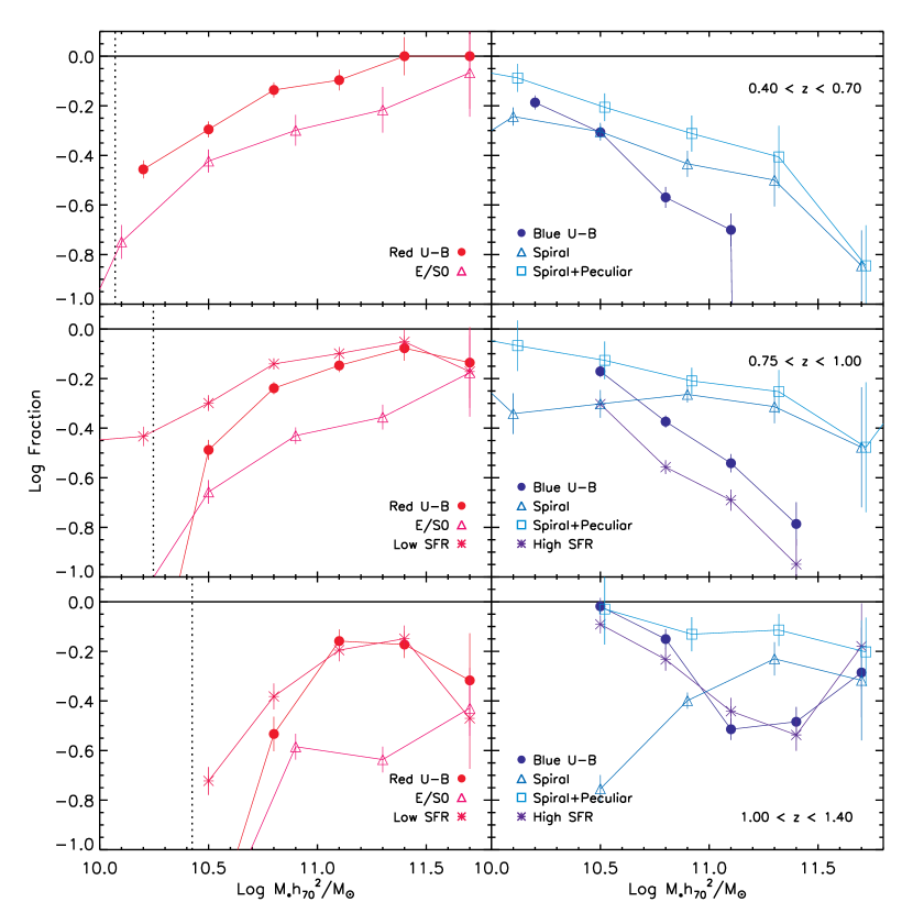
Figure 8.— Fractional contribution in log units to the total mass function from quiescent (left-hand plots) and active populations (right-hand plots) defined by rest-frame $(U-B)$ color, [OII] star formation rate, and morphology (see text for details). Star formation rates based on [OII] are only available for galaxies with $z>0.75$. The morphological mass functions are those of Bundy et al. (2005). The K_s-band completeness limits are indicated as in Figure 6.

The patterns in Figure 6 and 7 are also apparent when the galaxy population is partitioned by other indicators of star formation. This is demonstrated in Figure 8 which shows the fractional contribution (in log units) of active and quiescent populations to the total mass function. The “blue” and “red” samples defined by restframe $(U-B)$ color and shown in Figure 6 are reproduced here and indicated by solid circles.

For the two redshift intervals with $z>0.75$, we have plotted contributions from samples with high and low [OII]-derived SFRs. We divide this sample at 0.2 M_⊙ yr^-1, which is the median SFR of the star-forming population at $0.75<z<1.0$. This imposes a more stringent criterion than the restframe $(U-B)$ cut, which counts galaxies with only moderate or even recent star formation as “late-type.” Not surprisingly, the middle redshift bin contains fewer high-SFR galaxies compared to blue $(U-B)$ systems and more low-SFR galaxies than red systems, although the mass-dependence observed with either criteria is qualitatively similar.

In the high-$z$ bin, the populations defined by color and [OII] track each other more closely. Not only does this confirm that the mass-dependent evolution seen in Figure 6 is reproduced when the sample is divided by the [OII] SFR, but it also indicates that the average star formation rate is higher in this redshift bin. More of the “blue” population is now above the SFR cut as compared to the middle redshift bin. This evolution in the observed SFR will be discussed in detail in Noeske et al. (in preparation).

It is helpful also to understand how these trends relate to earlier work motivated by understanding the role of morphology in downsizing. Figure 8 also plots the contribution from morphologically-defined populations, drawing from the sample of Bundy et al. (2005) which has been adjusted to the $h=0.7$ cosmology used here (we note that the recent addition of HST/ACS imaging in the EGS provides an opportunity to extend this morphological comparison in the future). In Bundy et al. (2005), morphologies were determined visually using HST/ACS imaging data from the GOODS fields (Giavalisco et al., 2004) and were divided into three broad classes: E/S0, spirals, and peculiars. The fractional contribution from the spiral and spiral+peculiar samples are plotted in Figure 8 for comparison to the late-type populations described above. The E/S0 fraction is compared to the early-types. It should be noted that the smaller sample size of the Bundy et al. (2005) data leads to greater uncertainties and larger effects from cosmic variance.

With these caveats, there is quite good agreement in the mass-dependent evolutionary trends between the morphological and color/SFR selected samples. In detail, the fraction of ellipticals is systematically lower than the red/low-SFR populations while the fraction of spirals+peculiars is systematically higher than the blue/high-SFR galaxies. This suggests that the process that quenches star formation and transforms late-types into early-types operates on a longer timescale for morphology than it does for color or SFR. We return to this point in $\S$6. We also note that spiral galaxies do not always exhibit star formation and can be reddened by dust while some ellipticals have experienced recent star formation (e.g., Treu et al., 2005) that could lead to bluer colors.

5.4. Quantifying Downsizing: the Quenching Mass Threshold, $M_{Q}$

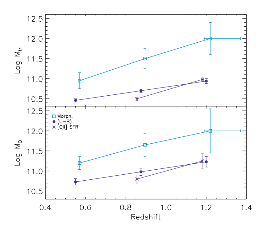
Figure 9.— Redshift evolution of the characteristic transitional mass, $M_{tr}$ (top plot), as well as the quenching mass, $M_{Q}$ (bottom plot). The plotted redshift values indicate the approximate average redshift in each bin. In both plots, the observed behavior is shown for the population partitioned according to morphology (light, open squares), restframe $(U-B)$ color (solid circles), and [OII] SFR (asterisks).

Several authors have identified a characteristic transition mass, $M_{tr}$, which divides the galaxy stellar mass function into a high-mass regime in which early-type, quiescent galaxies are dominant and a low-mass regime in which late-type, active galaxies are dominant (e.g., Kauffmann et al., 2003b; Baldry et al., 2004; Bundy et al., 2005). Using our various criteria, the downward evolution of this transitional mass with time is clearly demonstrated in the upper panel of Figure 9. For the color based mass functions, good agreement is found in comparison to the COMBO17 results discussed in (Borch et al., 2006). The morphological sample is taken from Bundy et al. (2005), where we have grouped spirals and peculiars into one star-forming population and compared its evolution to E/S0s. In the high-$z$ bin, $M_{tr}$ for the morphological sample occurs beyond the probed stellar mass range and so we have extrapolated to higher masses to estimate its value (this uncertainty is reflected in the horizontal error bar at this data point).

The color-defined $M_{tr}$ shows a redshift dependence of $M_{tr}\propto(1+z)^{4}$, similar to that for the morphological sample. Stronger evolution is seen for the the [OII]-defined samples as expected if evolution is more rapid for the most active sources. As discussed in $\S$5.3, the mass scale of morphological evolution is approximately 3 times larger ($\approx$0.5 dex) than that defined by color or [OII]. We also note from Figure 6 that $M_{tr}$ does not change appreciably when the $R$-band mass incompleteness is corrected in the high-$z$ bin.

While the evolution in $M_{tr}$ is illustrative of downsizing, since its definition in terms of physical processes is completely arbitrary (equality in the relative mass contributions of two populations), its significance is not clear. We prefer to seek a quantity that clearly describes the physical evolution taking place. Accordingly, we introduce and define a quenching mass limit, $M_{Q}$, as that mass above which star formation is suppressed in galaxies. This threshold is a direct byproduct of the mechanism that drives downsizing. We define $M_{Q}$ by noting the mass at which a line fit to the declining fraction of star-forming galaxies (Figure 7) drops below 1/3. We apply this simple definition to the other measures of star-forming populations and plot the resulting values of $M_{Q}$ in the bottom panel of Figure 9 and list them in Table 3. The relative behavior of differently classified populations is similar to the top panel, but the physical mass scale associated with $M_{Q}$ is a factor of 2–3 higher than that of $M_{tr}$. We find an approximate redshift dependence of $M_{Q}\propto(z+1)^{4.5}$, similar to the dependence of $M_{tr}$.

$M_{Q}$ is a useful quantity because it reveals the masses at which quenching operates effectively as a function of redshift. What is more, blue and star-forming galaxies at the quenching mass also tend to be among the reddest and least star-forming as compared to the full late-type population as a whole at each redshift, suggesting such galaxies are in the process of becoming early-types. As we discuss below, the quantitative evolution of $M_{Q}$ strongly constrains what mechanism or mechanisms quench star formation and also provides a convenient metric for testing galaxy formation models.

Table 3The Quenching Mass Threshold, $M_{Q}$

Redshift	Blue $(U-B)$	High SFR	Spirals+Peculiars
$0.4<z<0.7$	$10.73\pm 0.08$	—	$11.20\pm 0.16$
$0.75<z<1.0$	$10.98\pm 0.09$	$10.80\pm 0.10$	$11.65\pm 0.29$
$1.0<z<1.4$	$11.23\pm 0.13$	$11.25\pm 0.18$	$12.00\pm 0.55$

Note. — $M_{Q}$ is given in units of $\log(Mh_{70}^{2}/M_{\odot})$. Morphology data comes from Bundy et al. (2005).

5.5. The Environmental Dependence of Downsizing

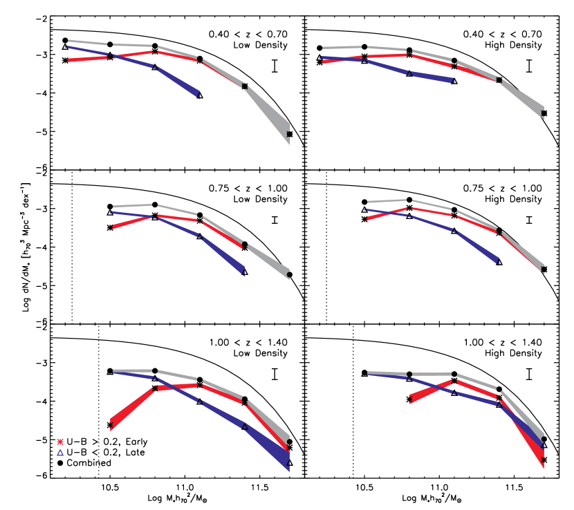
Figure 10.— Stellar mass functions in the three redshift bins at above- and below-average density partitioned by rest-frame $(U-B)$ color. The vertical dotted lines show the K_s-band magnitude completeness limits. The estimated cosmic variance is designated by the isolated error bar. Significant incompleteness from the $R$-band limit is expected in the high redshift bin, but it is not possible to apply corrections as in Figure 6 because the local density can only be measured in the spectroscopic sample. The solid line shows the Schechter fit to the photo-$z$ supplemented total mass function in our lowest redshift bin.

We have so far considered the mass-dependent evolution of late- and early-type populations integrated over the full range of environments probed by the DEEP2 Redshift Survey. We now divide the sample by environmental density to investigate how this evolution depends on the local environment.

In Figure 10, we plot galaxy stellar mass functions for the samples shown in Figure 6, split into low-density environments on the left-hand side and high-density environments on the right-hand side. The density discriminant is simply the median density (indicated by an overdensity of zero in Figure 2), so all galaxies are included. The evolution of the total mass functions in the two density regimes follows similar patterns as for the combined sample in Figure 6. Furthermore, the relative contribution of active and quiescent galaxies, as quantified by $M_{tr}$ and $M_{Q}$, exhibit the same kind of downsizing signal seen in Figure 6. Crucially, there is little difference (less than 25%) in the value of $M_{tr}$ between the below- and above-average density samples.

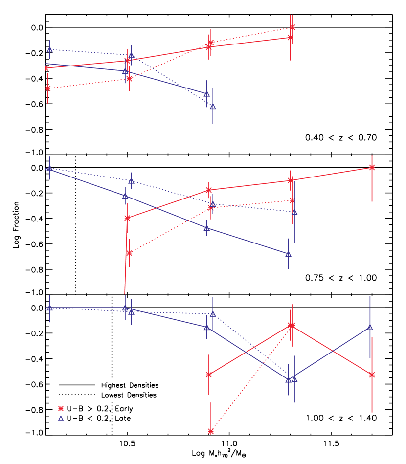
Figure 11.— Fractional contribution in log units to the total mass function. In each of three redshift bins solid lines connect points representing the extreme high-end of the density distribution, while dotted lines indicate the extreme low-end. The K_s-band completeness limits are indicated as vertical dotted lines.

The absence of a strong environmental trend in the downsizing pattern of massive galaxies is a surprising result that warrants further scrutiny. Although no strong dependence was seen in the Fundamental Plane analysis of Treu et al. (2005), their density estimates were much coarser and based on photometric redshifts. Local work utilizing the SDSS by Kauffmann et al. (2004) demonstrated differences in galaxy properties as a function of environment, but covered a much larger dynamic range in density than is accessible with our sample. We emphasize that the results of this work focus primarily on field galaxies, and, with the typical volumes probed ($\sim$10⁶ Mpc³), only rich groups are included at the highest densities. DEEP2 is too small to probe cluster scales.

It is important to note that individual density measurements, even in our spectroscopic analysis, can exhibit uncertainties of a factor of 3, so there is some overlap expected between the above- and below-average density regimes in Figure 6. However, because the total mass functions exhibit different abundances—with a factor of $\sim$2 more high-mass galaxies in the above-average density regime—the above- and below-average density subsamples successfully probe different populations. The higher abundance of massive galaxies at increasing densities agrees well with trends in local studies (e.g., Balogh et al., 2001, 2004; Baldry et al., 2004; Kauffmann et al., 2004).

Still, the comparison above is inevitably dominated by galaxies near the median density (Figure 2), and so we adopt a second, more stringent approach that divides the distribution into three, more extreme density bins. In this way, we can sample the full dynamic range of our survey. As described in $\S$3.3, we define a second set of density thresholds at $\pm$0.5 dex from the median density and construct mass functions for the extreme high- and low-density regimes. We plot the results in Figure 11, which again shows the fractional contribution of the red and blue populations to the total mass function. This time, the samples are also divided by density, with the high density points connected by solid lines and the low density points connected by dotted lines.

Figure 11 illustrates a more substantial environmental effect in the mass-dependent evolution of the sample that in each redshift interval is suggestive of local environmental trends (e.g., Kauffmann et al., 2004). Our observations allow us to investigate how these trends evolve with time. We find that the rise of the quiescent population and the evolution of $M_{tr}$ appears to be accelerated in regions of high environmental density. This effect does not depend on the particular choice of the density threshold, although the differences between the two environments grow as more of the sample near the median density is excluded from the analysis. The difference in $M_{tr}$ between these two environments is roughly a factor of 2–3. We caution that interpreting the results in the high-$z$ bin is difficult because the effects of completeness and weighting are most important here. However, the fact that the $M_{tr}$ values in the two density regimes are more similar in the high-$z$ bin (an offset of $\sim$0.1 dex) might suggest that the structural development or physical processes that lead to the density dependence at lower redshifts are not fully in place before $z\sim 1$.

The environmental dependence observed in Figure 11 does not occur because of the high-density regime alone, as one might expect given the potential presence of dense structures in the sample. The environmental effect is less strong but still apparent in comparisons between the high and middle density regimes as well as between the middle and low density regimes.

In summary, our various measures of downsizing, $M_{tr}$ and $M_{Q}$, depend strongly on redshift (they evolve by factors of $\sim$3–5 across the full redshift range), but less so on environmental density for most field galaxies (less than 25%). In support of previous inferences on the role of environment based on local studies (e.g., Balogh et al., 2004; Kauffmann et al., 2004; Blanton et al., 2004), this direct measurement of density-dependent evolution is particularly striking and serves to emphasize that galaxy mass, not environmental location, is the primary parameter governing the suppression of star formation and hence producing the signature of downsizing.

6. Discussion

6.1. The Rise of Massive Quiescent Galaxies

Figures 6 and 7 demonstrate a clear feature of the downsizing signal observed since $z\sim 1$, namely the increase in the number density of massive quiescent galaxies. Although our results are consistent with previous studies which found a rise in the red galaxy abundance of a factor of $\approx$2–6, depending on mass (Bell et al., 2004), the present work represents a significant step forward not only in its statistical significance and precision by virtue of access to the large spectroscopic and infrared data set, but also in clearly defining the mass-dependent trends.

In discussing our results we begin by considering the processes that might explain the present-day population of early-type galaxies. In order to reconcile the significant ages of their stellar populations implied by precise Fundamental Plane studies (e.g., Treu et al., 2005; van der Wel et al., 2005) with hierarchical models of structure formation, Bell et al. (2005a), Faber et al. (2005), van Dokkum (2005) and others have introduced the interesting possibility of “dry mergers”—assembly preferentially progressing via mergers of quiescent sub-units.

While dry mergers clearly occur (Tran et al., 2005; van Dokkum, 2005), our results suggest that they cannot be a substantial ingredient in the assembly history of massive quiescent galaxies. As shown in Figure 6, the observed increase in the number of quiescent systems is almost perfectly mirrored by a decline in star-forming galaxies such that the total mass function exhibits little evolution over $0.4<z<1.4$ compared to that of the red and blue populations. A simple transformation of one into the other is sufficient to high precision. For example, simply interchanging the numbers of red and blue galaxies in the high-$z$ bin in the mass range $10^{11.2}<\log{M_{*}/M_{\odot}}<10^{11.8}$, leads to a prediction for the number density in the middle-$z$ bin that is accurate to within $\sim$25%, well within the cosmic variance uncertainty. In addition, galaxies defined as blue or late-type with masses near $M_{Q}$ tend to be among the reddest and least star-forming, suggesting they are likely candidates for becoming early-type systems.

It is conceivable that the dry merger rate is mass-dependent and conspires to move galaxies along the mass function in a way that leaves its shape preserved. This would imply the presence of massive galaxies at low redshift that are not seen in our sample. For example, using the approximate dry merger rate estimate from Bell et al. (2005a) of 1.3 mergers every 6.3 Gyr, $\sim$25% of red galaxies would have to experience a major dry merger (in reality, this rate, calculated over $0<z<0.7$, might be expected to be higher at $z\sim 1$) between the high-$z$ and middle-$z$ bins. If we apply this rate of assembly to the red population in our high-$z$ bin at $\log(M_{*}/M_{\odot})=11.4$, we find that the total mass function in the middle-$z$ bin at $\log(M_{*}/M_{\odot})=11.7$ should be higher by approximately 60% compared to what is observed. While this one data point represents only a $\approx$2$\sigma$ result, similar arguments apply across the mass function and between the middle-$z$ and low-$z$ bins. More detailed modeling of the effect of merger rates on the mass function will be presented in a further paper (Bundy et al., in preparation).

Most difficult for the dry merger hypothesis as a key feature of galaxy formation is the weak environmental dependence we observe in the downsizing signal. Given a mechanism has to be found to preferentially bring quiescent sub-units together, one would expect a strong density dependence in the dry merger rate. By contrast, in our large sample it is clear that the majority of quiescent galaxies were assembled in a manner more sensitive to mass than environment.

Finally, our results show that downsizing is not only a feature of the star formation histories of massive quiescent galaxies (e.g., Treu et al., 2005; van der Wel et al., 2005), but is also apparent in the way their abundance increases. This observation is of particular interest for galaxy formation models based on the hierarchical $\Lambda$CDM framework. By incorporating AGN feedback effects into the semi-analytic models from the Munich group, De Lucia et al. (2005) predict star formation histories for massive ellipticals that follow the downsizing trend in which more massive galaxies host older stellar populations. However, as shown in Figure 5 from De Lucia et al. (2005), these models still predict a hierarchical mass assembly history for ellipticals. The problem in comparing the predictions of De Lucia et al. (2005) to our results (Figure 7, for example) is that the simulated ellipticals in De Lucia et al. (2005) are defined by their appearance at $z=0$, not the redshift at which we observe them. While the observations presented here suggest a top-down pattern in the growing abundance of early-types, it is not yet clear how significant a problem this may be for current semi-analytic models.

6.2. The Origin of Downsizing

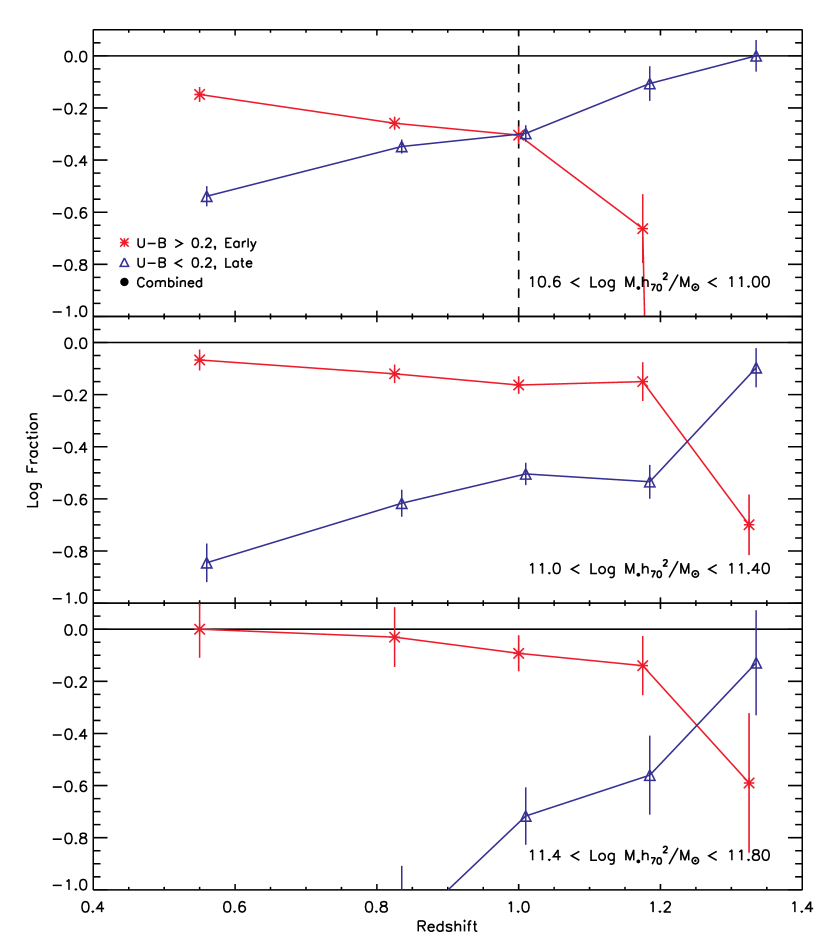
Figure 12.— Fractional contribution in log units to the total mass function, divided into stellar mass bins and plotted as a function of redshift. The plotted redshift values indicate the approximate average redshift in each bin. The vertical dashed line in the top panel indicates the onset of incompleteness from the $R$-band limit which occurs above the redshift indicated. The K_s-band completeness limit does not affect the results plotted in this figure.

The results of this paper reveal important clues as to the nature of downsizing and, via a clear measurement of the trends, will assist in constraining and ruling out several of the popular explanations. A detailed comparison with such models is beyond the scope of the current paper but we discuss some of the key issues here.

First we wish to dismiss a possible suggestion that our discovery of the quenching mass threshold is somehow an artifact of our selection process. For example, it might be argued that our result could arise from a uniform decrease in the incidence of star formation at all masses combined with a survey selection effect in which rare, massive objects are seen only at higher redshifts because of the larger volumes probed. Our results exclude this possibility. First, our sampled volumes are relatively similar (only a factor of $\sim$4 difference between low-$z$ and high-$z$), and we demonstrate that the fraction of star-forming galaxies depends not only on redshift but mass as well. Figure 12 illustrates this point. Here we divide the sample into smaller redshift intervals and follow the evolution of the red and blue populations in the three largest stellar mass bins, charting the fractional contribution of the two populations to the combined mass function. The highest mass bin contains the largest fraction of quiescent galaxies at almost every redshift, and the transformation of the active population into passively-evolving systems occurs first in the high mass bin and later at lower masses. The rate of change in the incidence of star formation is clearly mass-dependent.

Turning now to physical explanations, we have shown in $\S$5.4 that the quenching mass threshold, parametrized by $M_{Q}$, provides a very useful description of how the fraction of star-forming galaxies evolves. The question then is what mechanism is responsible for this quenching? Can it adequately reproduce the quantitative trends observed, for example the environmental dependence? Merging may provide a starting point for answering this question and explaining the transformation of late-types into early-types. Merging between disk systems has long been thought to be an important mechanism by which ellipticals form (e.g., Toomre, 1977; Barnes & Hernquist, 1991; Springel et al., 2005b) and the similar behavior of the morphological and color-defined values of $M_{Q}$ in Figure 9 suggests that the same process governing the growth of ellipticals may also broadly explain the rise of quiescent galaxies in general. However, as argued above, significant merging is likely to affect the shape of the total mass function which does not appear to evolve strongly in our sample. Merging may be occurring at masses below our completeness limit, but the observed evolution in the relative mix of early- and late-type galaxies suggests a process that quenches star formation first with morphological transformation following later. This would lead to higher values for $M_{Q}$ in the morphological samples, as observed.

Merger-triggered quenching has further difficulties. Fundamentally, the hierarchical merging of dark matter halos is expected to proceed from low mass to high mass, not the other way around. One solution to this difficulty would be to appeal to the fact that merging and assembly rates are accelerated in regions of high density (e.g., De Lucia et al., 2004) which also host the most massive systems. Over a range of environments, downsizing could arise naturally from the fact that massive galaxies live in these accelerated environments. However, we find no significant density dependence in the bulk of our sample (Figure 10), with downsizing appearing in all environments. This suggests that density-dependent merger rates are not the answer and that an internal feedback process on galactic scales is largely responsible for driving the downsizing pattern.

Many groups have recently suggested that internal AGN feedback may be the missing ingredient. Triggered perhaps by merging, energy deposited by the AGN effectively quenches further star formation, eventually transforming late-type galaxies into early-types (e.g., Silk & Rees, 1998). There are at least two current implementations of this process. In the explosive model, energy from an intense “quasar phase” (usually triggered by merging) heats and expels gas in the halo that would otherwise be available for star formation (Granato et al., 2004; Springel et al., 2005a; Scannapieco et al., 2005). While inspired by hydrodynamic simulations, it is not clear how the downsizing mass scale could arise from this model or what prevents future cooling of the expelled gas. In the “radio feedback” model, low luminosity AGN energy couples to hot gas in halos with masses greater than $M_{shock}$ in which the cooling time is longer than the dynamical time (see Dekel & Birnboim, 2004). This results in a long-term suppression of star formation in massive halos and, on even larger scales, cooling flows (e.g., Croton et al., 2005; De Lucia et al., 2005; Bower et al., 2005; Cattaneo et al., 2006). These models produce older stellar populations in more massive galaxies but still predict that low mass early-types (as defined at $z=0$) assemble first (see Figure 7). While a possible mass scale is provided in $M_{shock}$ that may help drive the downsizing signal, the physical mechanism that couples the radio feedback to the hot gas is not well understand. Beyond simulations and formation models incorporating AGN, additional evidence for the role of AGN feedback comes from phenomenological studies that relate observations of black hole mass, the quasar luminosity function, and the properties of galaxies in a consistent framework (e.g., Merloni et al., 2004; Hopkins et al., 2005; Merloni et al., 2006; Hopkins et al., 2006).

Regardless of the physical explanation for downsizing in the star formation activity of galaxies (and several may be necessary), it is clear that precise quantitative measures of the evolving mass distribution and its dependence on the basic parameters explored here will provide the ultimate test of these theories.

6.3. Reconciling Downsizing with the Hierarchical Structure Formation

In this section we step back from specific models of galaxy formation and explore in a more general sense the kinds of processes that may reconcile downsizing with hierarchical structure formation. Over the past decade there has been strong confirmation from many independent observations that the large-scale structure of the universe matches the basic predictions of the cold dark matter (CDM) model in which dark matter “halos” harbor galaxies and grow through constant, hierarchical merging with other halos. The masses of all halos increase monotonically with time, but at every epoch, it is the largest halos that are growing most actively and that are also the last to have assembled. Thus at first examination, downsizing, in which star formation proceeds from high-mass to low-mass systems, seem at odds with the CDM picture.

Several processes may be contributing to reversing the bottom-up trend in CDM structure formation to produce what appears to be a top-down pattern in galaxy formation. The first is a gradual effect resulting from the accelerating expansion of the universe which causes halo growth rates to slow once the universe reaches a scale factor $(1+z)^{-1}>\Omega_{m}$. The second is the physics of gas cooling, which selects a characteristic mass scale for galaxy formation (Rees & Ostriker, 1977; Silk, 1977; White & Rees, 1978). Gas cannot cool rapidly, and by implication stars cannot form efficiently, until structure formation produces halos with virial temperatures in excess of $10^{4}$ K . This sets the epoch for the onset of galaxy formation at $z\sim 15$–20. Once gas temperatures increase to $10^{6}$–$10^{7}$ K, cooling once again becomes inefficient, turning off star formation in the most massive halos. This then marks the end of galaxy formation, as more and more mass builds up in group and cluster halos above this cooling limit.

More detailed numerical or semi-analytic models of galaxy formation show that the cooling delay alone is insufficient to reduce star formation to observed levels, particularly in massive halos, and that other forms of feedback are required. While the details remain controversial (e.g., Benson et al., 2003), the net effect of this feedback is to place an upper limit on the range of halo masses over which active star formation can take place. This limit helps explain why star formation in galaxies is rarer at the present-day than it was at $z\sim$1–2. However, as discussed in $\S$6.2, it is less obvious how to explain the observed decline in the mass scale of star-forming galaxies.

To help gain insight into this question, we can attempt to relate various galaxies in our sample to dark matter halos. Models of the halo occupation distribution function predict that galaxies with the range of stellar masses sampled here ($\log(M/M_{\odot})\sim 10$–12, corresponding to $\log L_{b_{J}}\sim 10$–11.2) should reside in dark matter halos of mass $10^{12}$–$10^{15}M_{\odot}$ (e.g., Yang et al., 2003; Cooray & Milosavljević, 2005a), and furthermore that 75-80% of these galaxies will be “central,” that is the dominant galaxies within their halo, rather than satellites (Cooray & Milosavljević, 2005b). These models suggest that the objects in the three mass bins in Figure 12 correspond approximately to central galaxies in galaxy, group, and cluster halos.

In the top panel of Figure 13 we show the comoving number density of halos of mass $\log(M/M_{\odot})\,=\,12.5,13.5$ and 14.5 as a function of redshift (three lines, from top to bottom). The numbers are roughly consistent with the comoving number densities of galaxies in our three mass bins, although the most massive stellar objects are more abundant than $10^{14.5}M_{\odot}$ halos and may therefore reside in slightly less massive systems. The bottom panel shows the mean ages of halos in the three mass bins as a function of observed redshift. The mean age here is defined as the time elapsed since half of the halos in that mass range had first built up 90% or 50% of their current mass in a single progenitor (solid and dashed curves respectively), calculated using equation 2.26 from Lacey & Cole (1993).

By comparing Figure 13 to Figure 12 we can gain insight into the relationship between the assembly of dark matter halos and the process that drives the observed mass-dependent decline of star-forming galaxies. The fraction of the most massive blue galaxies declines from nearly 100% to $\sim$15% by $z\approx 1$ in Figure 12. For the least massive galaxies, this same decline lasts over the full redshift range of our sample, implying a timescale 2.5 times longer. Coupled with Figure 13—which indicates that the least massive halos in our sample are about twice the age of the most massive halos—this suggests a process that, for the low-mass systems, is at least 5 times slower than the growth of the dark matter halos in which they reside. Since global dynamical timescales should be independent of halo mass at a given redshift, this suggests that the quenching mechanism is strongly mass-dependent with the potential for different physical processes acting in different mass ranges.

Figure 13.— (Upper panel) The abundance of halos likely to host central galaxies in the three mass ranges plotted in Figure 12 versus redshift. The curves are labeled with $\log(M/M_{\odot})$. (Lower panel) Mean age of these systems as a function of their observed redshift. The mean age is defined as the time elapsed since half of the systems had built up a fraction $f$ of the mass they have at $z_{obs}$. Solid curves show the age for $f=0.9$ and dashed curves that for $f=0.5$.

7. Conclusions

Using a large sample that combines spectroscopy from the DEEP2 Galaxy Redshift Survey with panoramic near-IR imaging from Palomar Observatory, we have investigated the mass-dependent evolution of field galaxies over $0.4<z<1.4$. We have constructed stellar mass functions for active and quiescent populations, defined in several ways, and divided into different samples according to accurate measures of the environmental density determined from the extensive spectroscopic data. We summarize our conclusions below:

• The mass functions of active and quiescent galaxies integrated over all environments conclusively demonstrate a downsizing signal. We quantify this by charting the evolution in a “quenching mass,” $M_{Q}$, which describes the mass scale above which feedback processes suppress star formation in massive galaxies. We find that $M_{Q}\propto(1+z)^{3.5}$ with a factor of $\approx$3 decrease across the redshift range probed.

• The growth in the abundance of quiescent or “early-type” galaxies occurs first at the highest masses and then proceeds to lower mass systems. The relative abundance of early-types with $M_{*}\sim 10^{10}$M_⊙ has increased by a factor of $\approx$3 from $z\sim 1.2$ to $z\sim 0.55$, whereas the total mass function exhibits little evolution in shape and normalization (less than 0.2–0.3 dex). This implies that early-type systems result largely via the transformation of active star-forming galaxies, indicating that “dry mergers” are not a major feature of their assembly history.

• Alternative ways of dividing active and quiescent galaxies, including the use of [OII] equivalent widths and HST-derived morphologies, show qualitatively similar mass-dependent evolution and quenching. Interestingly, we observe that morphological evolution appears to take place on longer timescales than changes in the apparent star formation rate which operate at lower mass scales at each redshift.

• For the majority of galaxies in our sample, downsizing shows little dependence on environment. An environmental signal is apparent when the extremes of the density distribution are compared. In this case, downsizing in high-density regimes appears moderately accelerated compared to low-density ones, with values of $M_{tr}$ lower by a factor of $\sim$2.

• We discuss several possibilities for the origin of downsizing based on our results. We clearly rule out a scenario in which the incidence of star formation decreases uniformly for galaxies at all masses. The weak density dependence also argues against explanations that rely on the accelerated assembly of structure in dense environments, favoring internal mechanisms instead.

• Through comparisons to the expected behavior of dark matter halos, we argue that the dynamical timescale resulting from the growth of structure is at least 5 times longer in galaxies hosted by halos with $\log M/M_{\odot}\approx 12.5$ ($\log M_{*}/M_{\odot}\approx 10.8$) compared to $\log M/M_{\odot}=14.5$ ($\log M_{*}/M_{\odot}\approx 11.6$). Because global dynamical scales are also independent of halo mass at a given redshift, this suggests that the quenching mechanism is strongly mass-dependent with the potential for different physical processes acting in different mass ranges.

There are two obvious avenues for further studies of downsizing. In a forthcoming paper (Bundy et al., in preparation) we discuss the constraints on merging and the growth of galaxies determined by our observations of the total mass function. This will help dissect the role of merging in driving downsizing. In the near future, it will also be possible to chart the incidence of AGN among the galaxy population and compare it to the incidence of star formation to probe the link between quenching and AGN. The significant Chandra follow up observations currently underway in the EGS will make that field particularly exciting for such work. Other efforts from the DEEP2 collaboration have provided new insight on environmental trends (Cooper et al., 2006) and will focus on precise measures of the evolving star formation rate (Noeske et al., in preparation).

References

- Baldry et al. (2004) Baldry, I. K., Glazebrook, K., Brinkmann, J., Ivezić, Ž., Lupton, R. H., Nichol, R. C., & Szalay, A. S. 2004, ApJ, 600, 681
- Balogh et al. (2004) Balogh, M. L., Baldry, I. K., Nichol, R., Miller, C., Bower, R., & Glazebrook, K. 2004, ApJ, 615, L101
- Balogh et al. (2001) Balogh, M. L., Christlein, D., Zabludoff, A. I., & Zaritsky, D. 2001, ApJ, 557, 117
- Barnes & Hernquist (1991) Barnes, J. E. & Hernquist, L. E. 1991, ApJ, 370, L65
- Bauer et al. (2005) Bauer, A. E., Drory, N., Hill, G. J., & Feulner, G. 2005, ApJ, 621, L89
- Bell et al. (2003) Bell, E. F., McIntosh, D. H., Katz, N., & Weinberg, M. D. 2003, ApJS, 149, 289
- Bell et al. (2004) Bell, E. F., Wolf, C., Meisenheimer, K., Rix, H.-W., Borch, A., Dye, S., Kleinheinrich, M., Wisotzki, L., & McIntosh, D. H. 2004, ApJ, 608, 752
- Bell et al. (2005a) Bell, E. F. et al. 2005a, preprint (astro-ph/0506425)
- Bell et al. (2005b) —. 2005b, ApJ, 625, 23
- Benítez (2000) Benítez, N. 2000, ApJ, 536, 571
- Benson et al. (2003) Benson, A. J., Bower, R. G., Frenk, C. S., Lacey, C. G., Baugh, C. M., & Cole, S. 2003, ApJ, 599, 38
- Bertin & Arnouts (1996) Bertin, E. & Arnouts, S. 1996, A&AS, 117, 393
- Blanton et al. (2004) Blanton, M. R., Eisenstein, D. J., Hogg, D. W., & Zehavi, I. 2004, ArXiv Astrophysics e-prints
- Borch et al. (2006) Borch, A. et al. 2006, preprint (astro-ph/0604405)
- Bower et al. (2005) Bower, R. G. et al. 2005, ArXiv Astrophysics e-prints
- Brinchmann (1999) Brinchmann, J. 1999, Ph.D. Thesis
- Brinchmann & Ellis (2000) Brinchmann, J. & Ellis, R. S. 2000, ApJ, 536, L77
- Broadhurst et al. (1992) Broadhurst, T. J., Ellis, R. S., & Glazebrook, K. 1992, Nature, 355, 55
- Bruzual & Charlot (2003) Bruzual, G. & Charlot, S. 2003, MNRAS, 344, 1000
- Bundy et al. (2005) Bundy, K., Ellis, R. S., & Conselice, C. J. 2005, ApJ, 625, 621
- Cattaneo et al. (2006) Cattaneo, A., Dekel, A., Devriendt, J., Guiderdoni, B., & Blaizot, J. 2006, preprint (astro-ph/0601295)
- Chabrier (2003) Chabrier, G. 2003, PASP, 115, 763
- Cimatti et al. (2006) Cimatti, A., Daddi, E., & Renzini, A. 2006, preprint (astro-ph/0605353)
- Cimatti et al. (2002) Cimatti, A. et al. 2002, A&A, 392, 395
- Coil et al. (2004) Coil, A. L., Newman, J. A., Kaiser, N., Davis, M., Ma, C.-P., Kocevski, D. D., & Koo, D. C. 2004, ApJ, 617, 765
- Cole et al. (2000) Cole, S., Lacey, C. G., Baugh, C. M., & Frenk, C. S. 2000, MNRAS, 319, 168
- Cole et al. (2001) Cole, S. et al. 2001, MNRAS, 326, 255
- Collister & Lahav (2004) Collister, A. A. & Lahav, O. 2004, PASP, 116, 345
- Cooper et al. (2005) Cooper, M. C., Newman, J. A., Madgwick, D. S., Gerke, B. F., Yan, R., & Davis, M. 2005, preprint (astro-ph/0506518)
- Cooper et al. (2006) Cooper, M. C. et al. 2006, preprint (astro-ph/0603177), submitted
- Cooray & Milosavljević (2005a) Cooray, A. & Milosavljević, M. 2005a, ApJ, 627, L85
- Cooray & Milosavljević (2005b) —. 2005b, ApJ, 627, L89
- Cowie et al. (1999) Cowie, L. L., Songaila, A., & Barger, A. J. 1999, AJ, 118, 603
- Cowie et al. (1996) Cowie, L. L., Songaila, A., Hu, E. M., & Cohen, J. G. 1996, AJ, 112, 839
- Croton et al. (2005) Croton, D. J. et al. 2005, preprint (astro-ph/0508046)
- Cuillandre et al. (2001) Cuillandre, J.-C., Luppino, G., Starr, B., & Isani, S. 2001, in SF2A-2001: Semaine de l’Astrophysique Francaise, 605–+
- Davis et al. (2005) Davis, M., Gerke, B. F., Newman, J. A., & the Deep2 Team. 2005, in ASP Conf. Ser. 339: Observing Dark Energy, ed. S. C. Wolff & T. R. Lauer, 128–+
- Davis et al. (2003) Davis, M. et al. 2003, in Discoveries and Research Prospects from 6- to 10-Meter-Class Telescopes II. Edited by Guhathakurta, Puragra. Proceedings of the SPIE, Volume 4834, pp. 161-172 (2003)., 161–172
- De Lucia et al. (2005) De Lucia, G., Springel, V., White, S. D. M., Croton, D., & Kauffmann, G. 2005, preprint (astro-ph/0509725)
- De Lucia et al. (2004) De Lucia, G. et al. 2004, ApJ, 610, L77
- Dekel & Birnboim (2004) Dekel, A. & Birnboim, Y. 2004, preprint (astro-ph/0412300)
- Dickinson et al. (2003) Dickinson, M., Papovich, C., Ferguson, H. C., & Budavári, T. 2003, ApJ, 587, 25
- Dressler (1980) Dressler, A. 1980, ApJ, 236, 351
- Drory et al. (2004) Drory, N., Bender, R., Feulner, G., Hopp, U., Maraston, C., Snigula, J., & Hill, G. J. 2004, ApJ, 608, 742
- Drory et al. (2001) Drory, N., Feulner, G., Bender, R., Botzler, C. S., Hopp, U., Maraston, C., Mendes de Oliveira, C., & Snigula, J. 2001, MNRAS, 325, 550
- Drory et al. (2005) Drory, N., Salvato, M., Gabasch, A., Bender, R., Hopp, U., Feulner, G., & Pannella, M. 2005, ApJ, 619, L131
- Faber et al. (2003) Faber, S. M. et al. 2003, in Instrument Design and Performance for Optical/Infrared Ground-based Telescopes. Edited by Iye, Masanori; Moorwood, Alan F. M. Proceedings of the SPIE, Volume 4841, pp. 1657-1669 (2003)., 1657–1669
- Faber et al. (2005) Faber, S. M. et al. 2005, preprint (astro-ph/0506044)
- Flores et al. (1999) Flores, H. et al. 1999, ApJ, 517, 148
- Fontana et al. (2003) Fontana, A. et al. 2003, ApJ, 594, L9
- Fontana et al. (2004) —. 2004, A&A, 424, 23
- Gebhardt et al. (2003) Gebhardt, K. et al. 2003, ApJ, 597, 239
- Giavalisco et al. (2004) Giavalisco, M. et al. 2004, ApJ, 600, L93
- Granato et al. (2004) Granato, G. L., De Zotti, G., Silva, L., Bressan, A., & Danese, L. 2004, ApJ, 600, 580
- Guzman et al. (1997) Guzman, R., Gallego, J., Koo, D. C., Phillips, A. C., Lowenthal, J. D., Faber, S. M., Illingworth, G. D., & Vogt, N. P. 1997, ApJ, 489, 559
- Heavens et al. (2004) Heavens, A., Panter, B., Jimenez, R., & Dunlop, J. 2004, Nature, 428, 625
- Hopkins et al. (2006) Hopkins, P. F., Bundy, K., Hernquist, L., & Ellis, R. S. 2006, preprint (astro-ph/0601621)
- Hopkins et al. (2005) Hopkins, P. F., Hernquist, L., Cox, T. J., Robertson, B., & Springel, V. 2005, preprint (astro-ph/0508167)
- Jimenez et al. (2005) Jimenez, R., Panter, B., Heavens, A. F., & Verde, L. 2005, MNRAS, 356, 495
- Juneau et al. (2005) Juneau, S. et al. 2005, ApJ, 619, L135
- Kaiser et al. (1995) Kaiser, N., Squires, G., & Broadhurst, T. 1995, ApJ, 449, 460
- Kauffmann & Charlot (1998) Kauffmann, G. & Charlot, S. 1998, MNRAS, 297, L23+
- Kauffmann et al. (2004) Kauffmann, G., White, S. D. M., Heckman, T. M., Ménard, B., Brinchmann, J., Charlot, S., Tremonti, C., & Brinkmann, J. 2004, MNRAS, 353, 713
- Kauffmann et al. (2003a) Kauffmann, G. et al. 2003a, MNRAS, 341, 33
- Kauffmann et al. (2003b) —. 2003b, MNRAS, 341, 54
- Kewley et al. (2004) Kewley, L. J., Geller, M. J., & Jansen, R. A. 2004, AJ, 127, 2002
- Kinney et al. (1996) Kinney, A. L., Calzetti, D., Bohlin, R. C., McQuade, K., Storchi-Bergmann, T., & Schmitt, H. R. 1996, ApJ, 467, 38
- Lacey & Cole (1993) Lacey, C. & Cole, S. 1993, MNRAS, 262, 627
- Lilly et al. (1996) Lilly, S. J., Le Fevre, O., Hammer, F., & Crampton, D. 1996, ApJ, 460, L1+
- Maraston et al. (2006) Maraston, C., Daddi, E., Renzini, A., Cimatti, A., Dickinson, M., Papovich, C., Pasquali, A., & Pirzkal, N. 2006, preprint (astro-ph/0604530)
- Menci et al. (2005) Menci, N., Fontana, A., Giallongo, E., & Salimbeni, S. 2005, preprint (astro-ph/0506387)
- Merloni et al. (2004) Merloni, A., Rudnick, G., & Di Matteo, T. 2004, MNRAS, 354, L37
- Merloni et al. (2006) —. 2006, preprint (astro-ph/0602530)
- Nagashima & Yoshii (2004) Nagashima, M. & Yoshii, Y. 2004, ApJ, 610, 23
- Papovich et al. (2005) Papovich, C. et al. 2005, preprint (astro-ph/0511289)
- Rees & Ostriker (1977) Rees, M. J. & Ostriker, J. P. 1977, MNRAS, 179, 541
- Rudnick et al. (2003) Rudnick, G. et al. 2003, ApJ, 599, 847
- Scannapieco et al. (2005) Scannapieco, E., Silk, J., & Bouwens, R. 2005, preprint (astro-ph/0511116)
- Schmidt (1968) Schmidt, M. 1968, ApJ, 151, 393
- Shapley et al. (2005) Shapley, A. E., Steidel, C. C., Erb, D. K., Reddy, N. A., Adelberger, K. L., Pettini, M., Barmby, P., & Huang, J. 2005, ApJ, 626, 698
- Silk (1977) Silk, J. 1977, ApJ, 211, 638
- Silk & Rees (1998) Silk, J. & Rees, M. J. 1998, A&A, 331, L1
- Springel et al. (2005a) Springel, V., Di Matteo, T., & Hernquist, L. 2005a, ApJ, 620, L79
- Springel et al. (2005b) —. 2005b, MNRAS, 361, 776
- Toomre (1977) Toomre, A. 1977, in Evolution of Galaxies and Stellar Populations, 401–+
- Tran et al. (2004) Tran, K.-V. H., Franx, M., Illingworth, G. D., van Dokkum, P., Kelson, D. D., & Magee, D. 2004, ApJ, 609, 683
- Tran et al. (2005) Tran, K.-V. H., van Dokkum, P., Franx, M., Illingworth, G. D., Kelson, D. D., & Schreiber, N. M. F. 2005, ApJ, 627, L25
- Treu et al. (2005) Treu, T., Ellis, R. S., Liao, T. X., & van Dokkum, P. G. 2005, ApJ, 622, L5
- van der Wel et al. (2005) van der Wel, A., Franx, M., van Dokkum, P. G., Rix, H. ., Illingworth, G. D., & Rosati, P. 2005, preprint (astro-ph/0502228)
- van Dokkum (2005) van Dokkum, P. G. 2005, preprint (astro-ph/0506661)
- van Dokkum et al. (2000) van Dokkum, P. G., Franx, M., Fabricant, D., Illingworth, G. D., & Kelson, D. D. 2000, ApJ, 541, 95
- White & Rees (1978) White, S. D. M. & Rees, M. J. 1978, MNRAS, 183, 341
- Willmer (1997) Willmer, C. N. A. 1997, AJ, 114, 898
- Willmer et al. (2005) Willmer, C. N. A. et al. 2005, preprint (astro-ph/0506041)
- Wilson et al. (2002) Wilson, G., Cowie, L. L., Barger, A. J., & Burke, D. J. 2002, AJ, 124, 1258
- Wilson et al. (2003) Wilson, J. C. et al. 2003, in Instrument Design and Performance for Optical/Infrared Ground-based Telescopes. Edited by Iye, Masanori; Moorwood, Alan F. M. Proceedings of the SPIE, Volume 4841, pp. 451-458 (2003)., 451–458
- Wolf et al. (2003) Wolf, C., Meisenheimer, K., Rix, H.-W., Borch, A., Dye, S., & Kleinheinrich, M. 2003, A&A, 401, 73
- Wolf et al. (2004) Wolf, C. et al. 2004, A&A, 421, 913
- Yan et al. (2005) Yan, R., Newman, J. A., Faber, S. M., Konidaris, N., Koo, D., & Davis, M. 2005, preprint (astro-ph/0512446)
- Yang et al. (2003) Yang, X., Mo, H. J., & van den Bosch, F. C. 2003, MNRAS, 339, 1057