Spectral Methods for Time-Dependent Studies of Accretion Flows. II.
Two-Dimensional Hydrodynamic Disks with Self-Gravity

Abstract

Spectral methods are well suited for solving hydrodynamic problems in which the self-gravity of the flow needs to be considered. Because Poisson’s equation is linear, the numerical solution for the gravitational potential for each individual mode of the density can be pre-computed, thus reducing substantially the computational cost of the method. In this second paper, we describe two different approaches to computing the gravitational field of a two-dimensional flow with pseudo-spectral methods. For situations in which the density profile is independent of the third coordinate (i.e., an infinite cylinder), we use a standard Poisson solver in spectral space. On the other hand, for situations in which the density profile is a delta function along the third coordinate (i.e., an infinitesimally thin disk), or any other function known a priori, we perform a direct integration of Poisson’s equation using a Green’s functions approach. We devise a number of test problems to verify the implementations of these two methods. Finally, we use our method to study the stability of polytropic, self-gravitating disks. We find that, when the polytropic index $\Gamma$ is $\leq 4/3$, Toomre’s criterion correctly describes the stability of the disk. However, when $\Gamma>4/3$ and for large values of the polytropic constant $K$, the numerical solutions are always stable, even when the linear criterion predicts the contrary. We show that, in the latter case, the minimum wavelength of the unstable modes is larger than the extent of the unstable region and hence the local linear analysis is inapplicable.

1. Introduction

In the standard model of accretion disks, turbulent viscosity plays an important role in bringing material inward and transporting angular momentum outward (see Frank et al., 2002). At the same time, viscous dissipation converts gravitational potential energy to thermal energy and heats up the disk, which then radiates away this energy as thermal emission. In most applications of accretion disks around central objects, as in, e.g., X-ray binaries, the self-gravity of the flow is negligible compared to that of the central object. However, there are disk-like systems, such as active galactic nuclei as well as protostellar and protoplanetary disks, where the effects of self-gravity change not only the properties of angular momentum transport (Boss, 1998; Balbus & Papaloizou, 1999; Mejía et al., 2005), but also the energy balance equation (Bertin, 1997; Bertin & Lodato, 1999, 2001), which affect the global structure of the disk.

Besides the angular momentum transport problem, self-gravitating disks are also very important in studying star and planet formation. Indeed, gravitational instabilities in protoplanetary disks have been proposed as viable planet formation mechanisms. Although there has been a large amount of work done on gravitational instabilities in these system (see, for example, Pickett et al., 2003; Mejía et al., 2005, and references therein), it still remains an open question whether the fragmentation by gravitational instabilities can produce bound planetary objects, or if reservoirs of small solid cores are needed for the accretion mechanism to lead to rapid planet formation.

In the first paper in this series (Chan, Psaltis, & Özel 2005), we presented a pseudo-spectral method for solving the equations that describe the evolution of two dimensional, viscous hydrodynamic flows. There, we addressed issues related to the implementation of boundary conditions, spectral filtering, and time-stepping in spectral methods, and verified our algorithm using a suite of hydrodynamic test problems. In this second paper of the series, we present our implementation of a Poisson solver that allows us to take into account the effects of self-gravity of the flow.

Spectral methods are particularly suitable for incorporating the effects of self-gravity. Because Poisson’s equation is linear, we can pre-compute the numerical solution for the gravitational potential for each individual mode of the density, thus reducing substantially the computational cost of the method. In fact, Fourier methods have been used extensively in analytical studies of gravitational potentials in systems with periodic boundary conditions (Binney & Tremaine, 1987). On the other hand, in numerical studies of self-gravitating disks, the strengths of spectral methods have only been partially incorporated.

Hybrid hydrodynamic algorithms with self-gravity have been developed in such a way that modified spectral methods are used only for solving Poissson’s equation for the gravitational field, whereas the hydrodynamic parts are still treated with finite difference schemes. For example, Boss & Myhill (1992) describe a spherical harmonic decomposition method and a second-order scheme in the radial direction to solve Poisson’s equation, whereas Myhill & Boss (1993) use a modified Fourier method to find the gravitational potential of an isolated distribution of sources. Both algorithms employ explicit second-order finite difference methods to advance the hydrodynamic equations. Pickett et al. (1998, 2000) describe an implementation of an algorithm that uses Fourier decomposition in the azimuthal direction of cylindrical coordinate to solve Poisson’s equation together with a von Neumann & Richtmeyer AV scheme for the hydrodynamics. Some other examples can be found in Grandclement et al. (2001), Broderick & Rathore (2004), and Dimmelmeier et al. (2005). The main advantage of using hybrid methods is that one can employ currently available hydrodynamic algorithms based on finite difference schemes. However, a hybrid method does not exploit the high order of the spectral algorithm, because the hydrodynamic difference schemes typically have a much lower order compared to that of the Poisson solver. Contrary to these efforts, our algorithm uses a spectral decomposition method for solving both the hydrodynamic and Poisson’s equation, providing a consistent treatment of the whole problem. To our knowledge, this is the first time that spectral methods have been used in studying astrophysical disks with self gravity.

By construction, there is an ambiguity in the definition of the gravitational field in two-dimensional problems. We can assume either that the density profile is independent of the third coordinate (i.e., an infinite cylinder) or that it is a delta (or any other predetermined) function along the third coordinate (i.e., an infinitesimally thin disk); the resulting gravitational field on the two-dimensional domain of solution will be different in the two cases. For example, the gravitational potential of a “point source” on the two-dimensional domain of solution will be proportional to $\log(r)$ in the first case and to $1/r$ in the second, where $r$ is the distance from the source. In order to consider both geometries, here we describe two different approaches to computing the gravitational field of a two-dimensional hydrodynamic flow with pseudo-spectral methods. When the flow has the geometry of an infinite cylinder, we use a standard two-dimensional pseudo-spectral Poisson solver, which has been proven to be numerically stable and accurate. When the flow has the geometry of an infinitesimally thin disk, we perform a direct integration of the Green’s function for the gravitational potential, following the work of Cohl & Tohline (1999).

In the following section, we present our assumptions and equations. In §3, we discuss the details of our numerical methods, include both the standard Poisson solver and the Green’s function integrator. Next, we present a series of tests in §4, to verify our algorithm. Finally, we apply our method to a numerical study of Toomre’s stability criterion of self-gravitating disks in §5.

2. Equations and Assumptions

We consider two-dimensional, viscous, compressible flows. In this second paper, we include self-gravity and continue to neglect the magnetic fields of the flows. The hydrodynamic equations, therefore, contain the continuity equation

$$\frac{\partial\Sigma}{\partial t}+\nabla\cdot(\Sigma\mathbf{v})=0,$$ (1)

the Navier-Stokes equation

$$\Sigma\frac{\partial\mathbf{v}}{\partial t}+\Sigma(\mathbf{v}\cdot\nabla)\mathbf{v}=-\nabla P+\nabla\mathbf{\tau}+\Sigma\;\mathbf{g},$$ (2)

and the energy equation

$$\frac{\partial E}{\partial t}+\nabla\cdot(E\mathbf{v})=-P\,\nabla\cdot\mathbf{v}+\Phi-\nabla\cdot\mathbf{q}-\nabla\cdot\mathbf{F}-2F_{z}.$$ (3)

We denote by $\Sigma$ the height-integrated density, by $\mathbf{v}$ the fluid velocity, and by $E$ the thermal energy. In the Navier-Stokes equation, $P$ is the height-integrated pressure, $\mathbf{\tau}$ is the viscosity tensor, and $\mathbf{g}$ is the gravitational acceleration. We use $\Phi$ to denote the viscous dissipation rate, $\mathbf{q}$ to denote the heat flux vector, and $\mathbf{F}$ to denote the radiation flux on the $r$-$\phi$ plane. The last term in the heat equation, $2F_{z}$, takes into account the radiation losses in the vertical direction. The analytical forms of the various physical quantities in equations (1)–(3) are given in Chan et al. (2005), except for the gravitational acceleration $\mathbf{g}$, for which we need to introduce a new equation.

In Newtonian gravity, the gravitational field $\mathbf{g}$ is conservative, so we can define the gravitational potential $\Psi$ by

$$\mathbf{g}\equiv-\nabla\Psi.$$ (4)

The gravitational potential associated with the (three-dimensional) mass density, $\rho$, is given by the volume integral

$$\Psi(t,\mathbf{x})=-G\int\frac{\rho(t,\mathbf{x^{\prime}})}{|\mathbf{x}-\mathbf{x^{\prime}}|}d^{3}x^{\prime}$$ (5)

over all space, where $G$ is the gravitational constant. Rewriting equation (5) in differential form, we obtain Poisson’s equation

$$\nabla^{2}\Psi=4\pi G\rho,$$ (6)

with $\Psi$ satisfying the boundary condition $\Psi(t,\infty)=0$ at all times. When simulating astrophysical flows, the computational domain $\mathcal{D}^{(3)}$ is usually finite. Based on its linearity, we can decompose the Poisson equation into two parts

$$\nabla^{2}\Psi_{\mathrm{int}}=4\pi G\rho_{\mathrm{int}},$$ (7)

and

$$\nabla^{2}\Psi_{\mathrm{ext}}=4\pi G\rho_{\mathrm{ext}},$$ (8)

where $\rho_{\mathrm{int}}$ denotes the mass density within the computational domain, which in our case is the flow density, and $\rho_{\mathrm{ext}}$ refers to external sources such as a central object and/or a companion star. The gravitational field is then given by

$$\mathbf{g}=\mathbf{g}_{\mathrm{int}}+\mathbf{g}_{\mathrm{ext}}=-\nabla(\Psi_{\mathrm{int}}+\Psi_{\mathrm{ext}}).$$ (9)

In the astrophysical context of interest here, $\Psi_{\mathrm{ext}}$ is usually generated by a set of spherical objects. Hence the external gravitational potential is given by

$$\Psi_{\mathrm{ext}}(t,\mathbf{x})=\sum_{i}\frac{GM_{i}}{|\mathbf{x}-\mathbf{x}_{i}(t)|},$$ (10)

where $M_{i}$ and $\mathbf{x}_{i}(t)$ are the mass and positions of the corresponding objects. Regarding the self-gravity of the flow, solving equation (7) within $\mathcal{D}^{(3)}$ is equivalent to computing the integral

$$\Psi_{\mathrm{int}}(t,\mathbf{x})=-G\int_{\mathcal{D}^{(3)}}\frac{\rho_{\mathrm{int}}(t,\mathbf{x^{\prime}})}{|\mathbf{x}-\mathbf{x^{\prime}}|}d^{3}x^{\prime}.$$ (11)

Once $\Psi_{\mathrm{ext}}$ and $\Psi_{\mathrm{int}}$ are obtained, we can then use equation (9) to obtain the total gravitational field and subsequently use it in both the Navier-Stokes equation and in integrating the trajectories $\mathbf{x}_{i}(t)$ for the external objects. Although for our test problems we assume that the central object does not move and solve the hydrodynamic equations in a fixed reference frame, it is trivial to generalize our algorithm to co-moving coordinates.

There are two different approaches to reducing the above three-dimensional formalism to two dimensions, depending on the physical problem under study. The first one assumes that the density is independent of the vertical coordinate $z$, i.e., $\rho_{\mathrm{int}}(t,r,\phi,z)\equiv\rho_{\mathrm{ind}}(t,r,\phi)$. In this case, we define $\psi(t,r,\phi)\equiv\Psi_{\mathrm{int}}(t,r,\phi,z)$ and we are left with a two-dimensional problem. We obtain the gravitational potential by solving the two-dimensional Poisson’s equation

$$\nabla^{2}\psi\equiv\left(\frac{\partial^{2}}{\partial r^{2}}+\frac{\partial}{r\partial r}+\frac{\partial^{2}}{r^{2}\partial\phi^{2}}\right)\psi=4\pi G\rho_{\mathrm{ind}}$$ (12)

(This approach is used in ZEUS-2D, see Stone & Norman, 1992, for details.)

The second approach assumes that the vertical structure of the density is described by some function $Z(r,z)$ that is independent of $t$ and $\phi$, i.e., $\rho_{\mathrm{int}}(t,r,\phi,z)\equiv\Sigma(t,r,\phi)Z(r,z)$. We are interested in the gravitational potential on the $z=0$ plane, so that we solve for $\psi(t,r,\phi)=\Psi_{\mathrm{int}}(t,r,\phi,z=0)$. This is a “pseudo-two-dimensional” problem, where the potential is not described by a two-dimensional Poisson equation. In order to compute the potential properly, the easiest method, in this case, is to integrate directly the equation

$$\psi(t,r,\phi)=\int_{\mathcal{D}^{(2)}}\mathcal{G}(r,\phi;r^{\prime},\phi^{\prime})\Sigma(t,r^{\prime},\phi^{\prime})r^{\prime}dr^{\prime}d\phi^{\prime},$$ (13)

where $\mathcal{D}^{(2)}$ denotes the two-dimensional computational domain and

$$\mathcal{G}(r,\phi;r^{\prime},\phi^{\prime})\equiv-G\int_{-\infty}^{\infty}\frac{Z(r^{\prime},z^{\prime})dz^{\prime}}{\sqrt{r^{2}+r^{\prime 2}-2rr^{\prime}\cos(\phi-\phi^{\prime})+z^{\prime 2}}}$$ (14)

is the “modified Green’s function” for our problem.

3. Numerical Methods

In this section, we describe the numerical methods we use to solve the two classes of self-gravity problems. As in the first paper (Chan et al., 2005), we use pseudo-spectral methods, in which we expand all functions in series by choosing the truncated functions to agree with the approximated functions exactly at the grid points.

We use the modified Chebyshev collocation method along the radial direction and the Fourier collocation method along the azimuthal direction. Let $N+1$ and $M$ be the number of collocation points in the radial and azimuthal direction, respectively. For every function $f(r,\phi)$, we use the subscript $m$ to indicate the Fourier coefficients

$$f(r,\phi)=\sum_{m=-M/2}^{M/2-1}\hat{f}_{m}(r)e^{im\phi}$$ (15)

and the subscript $n$ to indicate the Chebyshev-Fourier coefficients

$$f(r,\phi)=\sum_{n=0}^{N}\sum_{m=-M/2}^{M/2-1}\check{f}_{nm}T_{n}(\bar{r})e^{im\phi},$$ (16)

where $\bar{r}\in[-1,1]$ denotes the standardized coordinate (see Chan et al., 2005, for notation).

We implement a standard two-dimensional pseudo-spectral Poisson solver, which we describe briefly in §3.1 (a good introduction is available in Trefethen, 2000). For the direct integrator, we describe in §3.2 how to generalize the compact cylindrical Green’s function expansion (Cohl & Tohline, 1999) with pseudo-spectral methods. Both methods use pre-computed matrices to speed up the algorithms. The run-time computational cost for both methods are of order $\mathcal{O}(N^{2}M+NM\log_{2}M)$.

3.1. Two-Dimensional Pseudo-Spectral Poisson Solver

We describe here a two-dimensional, pseudo-spectral Poisson solver. We use the fact that the basis polynomials in the $\phi$ direction, $e^{im\phi}$, are also eigenfunctions of the operator $\partial^{2}/\partial\phi^{2}$ in order to split the Poisson’s equation to

$$\Delta_{m}\hat{\psi}_{m}\equiv\left(\frac{\partial^{2}}{\partial r^{2}}+\frac{\partial}{r\partial r}-\frac{m^{2}}{r^{2}}\right)\hat{\psi}_{m}=\hat{f}_{m}$$ (17)

for $m=0,1,\dots,M/2$, where we have set $f\equiv 4\pi G\rho_{\mathrm{ind}}$. Note that, in discrete Fourier transforms, $\hat{f}_{0}$ and $\hat{f}_{M/2}$ are real but the other coefficients are complex, so there are, in total, $M$ independent equations. We use $\Delta_{m}$ to denote the differential operator for each $m$. In the case of the $r-$direction, the Chebyshev polynomials are not eigenfunctions of $\Delta_{m}$. Nevertheless, because $\Delta_{m}$ is time independent and linear, we can write $\Delta_{m}$ in matrix representation and pre-compute its inverse $\Delta_{m}^{-1}$ with an $\mathcal{O}(N^{2})$ solver for each $m$.

Let $\bar{r}$ be the standardized coordinate of Chebyshev polynomials and $r=g(\bar{r})$ be the mapped (physical) coordinate (see Chan et al., 2005, for more details). It is well known that the spectral Chebyshev derivative in the standardized coordinate can be written in matrix representation as

$$\bar{D}_{ij}=\left(\begin{array}[]{c|ccc|c}\frac{2N^{2}+1}{6}&\cdots&2\frac{(-1)^{j}}{1-x_{j}}&\cdots&\frac{1}{2}(-1)N\\ \hline\cr\vdots&\ddots&&\frac{(-1)^{i+j}}{x_{i}-x_{j}}&\vdots\\ -\frac{1}{2}\frac{(-1)^{i}}{1-x_{i}}&&\frac{-x_{j}}{2(1-x_{j}^{2})}&&-\frac{1}{2}\frac{(-1)^{N+i}}{1+x_{i}}\\ \vdots&\frac{(-1)^{i+j}}{x_{i}-x_{j}}&&\ddots&\vdots\\ \hline\cr-\frac{1}{2}(-1)N&\cdots&-2\frac{(-1)^{N+j}}{1+x_{j}}&\cdots&-\frac{2N^{2}+1}{6}\end{array}\right),$$ (18)

which is a $(N+1)\times(N+1)$ matrix (discussion of computing this matrix accurately can be found in Baltensperger & Trummer, 2003). The derivative in the mapped coordinate can be obtained by the chain rule

$$\frac{\partial}{\partial r}=\frac{d\bar{r}}{dr}\frac{\partial}{\partial\bar{r}}=\frac{1}{dg/d\bar{r}}\frac{\partial}{\partial r},$$ (19)

so that the derivative matrix in the mapped coordinate is given by the product

$$D_{ij}\equiv\frac{1}{(dg/d\bar{r})|_{\bar{r}_{i}}}\bar{D}_{ij}.$$ (20)

With this we are able to write

$$\Delta_{m,ij}=\sum_{k}D_{ik}D_{kj}+\sum_{k}\frac{\delta_{ik}}{x_{i}}D_{kj}-\frac{\delta_{ij}}{x_{i}^{2}}m^{2}.$$ (21)

The matrix $\Delta_{m,ij}$ is, of course, singular because a unique solution to $\psi_{m}$ does not exist until the boundary conditions are given.

An important case is the vanishing boundary condition $\hat{\psi}_{m}(r_{\min})=\hat{\psi}_{m}(r_{\max})=0$. Let $\tilde{\Delta}_{m,ij}$ be the $(N-1)\times(N-1)$ sub-matrix of $\Delta_{m,ij}$ generated by removing the first and last rows and columns. Imposing the vanishing boundary condition to $\Delta_{m,ij}^{-1}$ is then equivalent to finding the inverse of the $\tilde{\Delta}_{m,ij}$ and filling back the first and last rows and columns with zeros, i.e.,

$$\Delta^{-1(0)}_{m,ij}=\left(\begin{array}[]{c|ccc|c}0&0&\cdots&0&0\\ \hline\cr 0&&&&0\\ \vdots&&\tilde{\Delta}_{m,ij}^{-1}&&\vdots\\ 0&&&&0\\ \hline\cr 0&0&\cdots&0&0\end{array}\right).$$ (22)

We can then calculate

$$\hat{\psi}^{(0)}_{m}(r_{i})=\sum_{j=0}^{N}\Delta_{m,ij}^{-1(0)}\hat{f}_{m}(r_{j}),$$ (23)

where the superscript $(0)$ indicates that the solutions satisfy the homogeneous boundary conditions for all $m$. Taking the inverse Fourier transform along the $\phi$-direction, we then obtain the solution $\psi^{(0)}(r,\phi)$ which satisfies the vanishing boundary conditions.

In order to apply more generic boundary conditions, we first look for solutions $\hat{\psi}^{(1)}_{m}(r)$ that satisfy the homogeneous differential equation

$$\Delta_{m}\hat{\psi}^{(1)}_{m}=0$$ (24)

with the proper boundary conditions. Then it is clear that the sum $\hat{\psi}^{(0)}_{m}+\hat{\psi}^{(1)}_{m}$ satisfies

$$\Delta_{m}\left(\hat{\psi}^{(0)}_{m}+\hat{\psi}^{(1)}_{m}\right)=\hat{f}_{m}$$ (25)

with the same boundary conditions. The solutions to equation (24) are

$$\hat{\psi}^{(1)}_{m}(r)=\left\{\begin{array}[]{lll}C_{m}\ln r+D_{m}&,&m=0\\ C_{m}r^{m}+D_{m}r^{-m}&,&m=1,2,\dots,M/2\end{array}\right.$$ (26)

where $C_{m}$ and $D_{m}$ are complex constants, which are fixed by the boundary conditions. In general, these boundary conditions depend on azimuth, i.e.,

$$\psi(r_{\min},\phi) = \beta_{\mathrm{in}}(\phi),$$ (27)

$$\psi(r_{\max},\phi) = \beta_{\mathrm{out}}(\phi).$$ (28)

We first take the Fourier transform of $\beta_{\mathrm{in}}(\phi)$ and $\beta_{\mathrm{out}}(\phi)$, we solve for $C_{m}$ and $D_{m}$ using

$$\hat{\beta}_{\mathrm{in},m} = \left\{\begin{array}[]{lll}C_{m}\ln r_{\min}+D_{m}&,&m=0\\ C_{m}r_{\min}^{m}+D_{m}r_{\min}^{-m}&,&m=1,2,\dots,M/2\end{array}\right.$$ (31)

$$\hat{\beta}_{\mathrm{out},m} = \left\{\begin{array}[]{lll}C_{m}\ln r_{\min}+D_{m}&,&m=0\\ C_{m}r_{\min}^{m}+D_{m}r_{\min}^{-m}&,&m=1,2,\dots,M/2,\end{array}\right.$$ (34)

we add these terms to $\hat{\psi}^{(0)}_{m}$, and finally take the inverse Fourier transform.

We summarize the two-dimensional pseudo-spectral Poisson solver using the following steps:

1. We take the Fourier transform of each physical quantity $f$ along the $\phi$-direction and obtain $\hat{f}_{m}$ by a fast Fourier transform, which is of order $\mathcal{O}(NM\log_{2}M)$.

2. We then compute the matrix product (23) for each $m$, which is of order $\mathcal{O}(N^{2}M)$.

3. We compute $\hat{\beta}_{m}$ by a fast Fourier transform, which is of order $\mathcal{O}(M\log_{2}M)$.

4. We then solve for $C_{m}$ and $D_{m}$ using equations (31) and (34), which is of order $\mathcal{O}(M)$.

5. We impose the boundary conditions using equation (26), for each $m$, and obtain $\hat{\psi}_{m}(r_{k})$, which is of order $\mathcal{O}(NM)$.

6. Finally, we take the inverse transform of $\hat{\psi}_{m}$ to obtain the potential $\psi$, which is of order $\mathcal{O}(NM\log_{2}M)$.

Therefore, the overall computational cost is $\mathcal{O}(N^{2}M+NM\log_{2}M)$.

3.2. Two-Dimensional Gravity Integrator

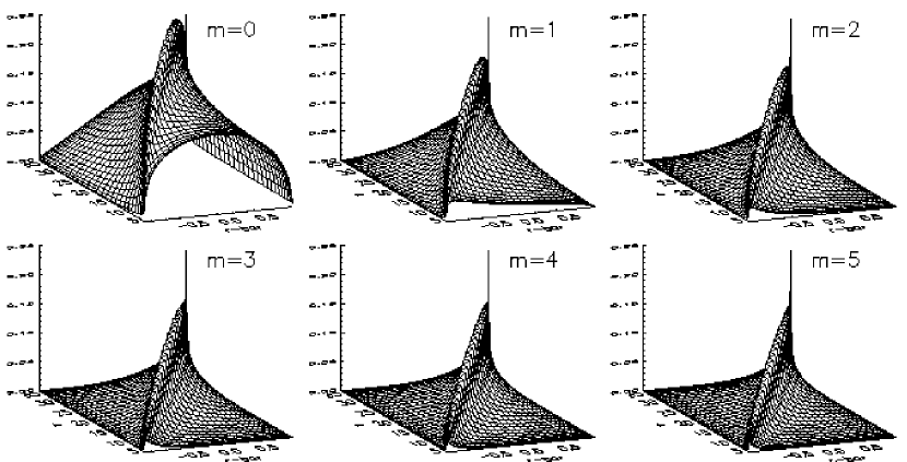
Figure 1.— Plots of the quantity $\mathcal{I}_{m}(\bar{r}^{\prime};r)$ for the first six values of $m$, when $N=33$, $M=64$, and $Z(r,z)=\delta(z)$.

As described in §2, we assume in this case that the vertical structure of the density is time-independent and has cylindrical symmetry. Hence we can write

$$\rho_{\mathrm{int}}(t,r,\phi,z)=\Sigma(t,r,\phi)Z(r,z),$$ (35)

where we normalize $Z(r,z)$ along the $z$ direction to unity, i.e.,

$$\int_{-\infty}^{\infty}Z(r,z)dz=1,$$ (36)

so that $\Sigma$ has the physical meaning of a height-integrated density.

We present here a new numerical method to compute the integral (13) efficiently and accurately. Our method is motivated by Cohl & Tohline (1999), who showed that the three-dimensional Green’s function in cylindrical coordinates can be expanded in the compact form

$$\frac{1}{|\mathbf{x}-\mathbf{x^{\prime}}|}\equiv\frac{1}{\pi\sqrt{rr^{\prime}}}\sum_{m=-\infty}^{\infty}e^{im(\phi-\phi^{\prime})}Q_{m-1/2}(\chi),$$ (37)

where $\chi\equiv[r^{2}+r^{\prime 2}+(z-z^{\prime})^{2}]/2rr^{\prime}$ and $Q_{m-1/2}(\chi)$ are the half-integer degree Legendre functions. Note that the $\phi$ and $\phi^{\prime}$ dependence appears only in the exponential $e^{im(\phi-\phi^{\prime})}$. This can be done because the Green’s function itself can be written as a function of $\Delta\phi=\phi-\phi^{\prime}$ so that $Q_{m-1/2}(\chi)/\pi\sqrt{rr^{\prime}}$ is simply the Fourier transform of $|\mathbf{x}-\mathbf{x^{\prime}}|^{-1}$ with respect to $\Delta\phi$. This property is still true for the modified Green’s function because $Z$ is $\phi$-independent:

$$\mathcal{G}(r,\phi\;;r^{\prime},\phi^{\prime})=\mathcal{G}(r,r^{\prime},\Delta\phi).$$ (38)

Expanding it in Fourier series, i.e.,

$$\mathcal{G}(r,\phi;r^{\prime},\phi^{\prime})=\sum_{m=-\infty}^{\infty}\hat{\mathcal{G}}_{m}(r,r^{\prime})e^{im(\phi-\phi^{\prime})},$$ (39)

and substituting it into equation (13), we obtain

$$\psi(r,\phi)=\int_{\mathcal{D}^{(2)}}\sum_{m=-\infty}^{\infty}\hat{\mathcal{G}}_{m}(r,r^{\prime})e^{im(\phi-\phi^{\prime})}\Sigma(r^{\prime},\phi^{\prime})r^{\prime}dr^{\prime}d\phi^{\prime}.$$ (40)

Note that the integration over $\phi^{\prime}$,

$$\int_{0}^{2\pi}d\phi^{\prime}\Sigma(r^{\prime},\phi^{\prime})e^{-im\phi^{\prime}}=2\pi\Sigma_{m}(r^{\prime}),$$ (41)

is the Fourier transform of $\Sigma(r^{\prime},\phi^{\prime})$ in the azimuthal direction. Therefore, we can rewrite equation (40) as

$$\psi(r,\phi)=\sum_{m=-\infty}^{\infty}\int_{r_{\min}}^{r_{\max}}\hat{\mathcal{G}}_{m}(r,r^{\prime})2\pi\hat{\Sigma}_{m}(r^{\prime})e^{im\phi}r^{\prime}dr^{\prime}.$$ (42)

Taking the Fourier transform of the whole equation again with respect to $\phi$, we obtain a one-dimensional integral for each value of $m$

$$\hat{\psi}_{m}(r)=\int_{r_{\min}}^{r_{\max}}\hat{\mathcal{G}}_{m}(r,r^{\prime})2\pi\hat{\Sigma}_{m}(r^{\prime})r^{\prime}dr^{\prime}.$$ (43)

We now expand $\hat{\Sigma}_{m}(r^{\prime})$ in Chebyshev polynomials, i.e.,

$$\hat{\Sigma}_{m}(r^{\prime})=\sum_{n=0}^{\infty}\check{\Sigma}_{nm}T_{n}(\bar{r}^{\prime}).$$ (44)

Recalling that $\bar{r}^{\prime}$ is the standardized coordinate, we let $r^{\prime}=g(\bar{r}^{\prime})$ be some coordinate mapping. Equation (43) can then be rewritten as

$$\hat{\psi}_{m}(r)=\sum_{n=0}^{\infty}\check{\Sigma}_{nm}\int_{r_{\min}}^{r_{\max}}\hat{\mathcal{G}}_{m}(r,r^{\prime})2\pi T_{n}(\bar{r}^{\prime})r^{\prime}dr^{\prime}.$$ (45)

Because the orthogonality condition of Chebyshev polynomials has a weight function $(1-\bar{r}^{\prime 2})^{-1/2}$, i.e.,

$$\langle T_{l},T_{n}\rangle=\int_{-1}^{1}\frac{T_{l}(\bar{r}^{\prime})T_{n}(\bar{r}^{\prime})}{\sqrt{1-\bar{r}^{\prime 2}}}d\bar{r}^{\prime}=\frac{\pi}{c_{n}}\;\delta_{ln},$$ (46)

where $c_{0}=2$ and $c_{n}=1$ for $n=1,2,\dots$, it is not difficult to see that, by defining

$$\hat{\mathcal{I}}_{m}(\bar{r}^{\prime};r)=\hat{\mathcal{G}}_{m}\left[r,g(\bar{r}^{\prime})\right]\pi\sqrt{1-\bar{r}^{\prime 2}}\;\frac{dg^{2}}{d\bar{r}^{\prime}},$$ (47)

we can write

$$\hat{\psi}_{m}(r) = \sum_{n=0}^{\infty}\check{\Sigma}_{nm}\int_{-1}^{1}\frac{\hat{\mathcal{I}}_{m}(\bar{r}^{\prime};r)T_{n}(\bar{r}^{\prime})}{\sqrt{1-\bar{r}^{\prime 2}}}d\bar{r}^{\prime}$$ (48)

$$= \sum_{n=0}^{\infty}\check{\Sigma}_{nm}\langle\hat{\mathcal{I}}_{m},T_{n}\rangle$$

$$= \sum_{n=0}^{\infty}\frac{\check{\Sigma}_{nm}\check{\mathcal{I}}_{nm}(r)}{c_{n}},$$

where $\check{\mathcal{I}}_{nm}(r)$ is the $n$-th Chebyshev coefficient of $\hat{\mathcal{I}}_{m}(\bar{r}^{\prime};r)$ with respect to $\bar{r}^{\prime}$.

Up to this point, although the function $\Sigma(r^{\prime},\phi^{\prime})$ has been written in Chebyshev-Fourier series, we have assumed that the series is infinite and hence the formalism is exact. In order to perform it numerically, we have to discretize equation (48).

For the azimuthal direction, which is periodic, we simply replace the continuous Fourier transform by a discrete Fourier transform and use the proper normalization, which does not change equation (48) but only limits the index $m$ to the range $-M/2$ to $M/2-1$. For the $r$-direction, we truncate the infinite sum at a finite number of terms, $N$. Therefore, equation (48) becomes

$$\hat{\psi}_{m}(r_{k})=\sum_{n=0}^{N}\frac{\check{\Sigma}_{nm}\check{\mathcal{I}}_{nm}(r_{k})}{c_{n}},$$ (49)

where $r_{k}$ denotes the collocation points in the $r$-direction.

Once we obtain $\check{\mathcal{I}}_{nm}(r_{k})$ for $n=0,1,\dots,N$, the calculation of the gravitational potential is trivial. However, note that $Q_{m-1/2}(\chi)$ is related to the complete elliptic integral, which is singular when $r^{\prime}=r_{k}$. In general, this difficulty arises because of the singularity of $|\mathbf{x}-\mathbf{x}^{\prime}|^{-1}$. In order to avoid the singularity, we use the “Chebyshev-roots grid”:

$$\bar{r}^{\prime}_{j}=\cos\left[\frac{(2j+1)\pi}{2N}\right],\ \ \ 0\leq j<N$$ (50)

so that $\hat{\mathcal{I}}_{m}(\bar{r}^{\prime}_{j};r_{k})$ is finite for all $m$ and $j$. In Figure 1, we plot $\hat{\mathcal{I}}_{m}(\bar{r}^{\prime};r)$ for the first six values of $m$ for $N=33$, $M=64$, and $Z(r,z)=\delta(z)$, which is the case of a very thin disk.

The Chebyshev coefficients $\check{\mathcal{I}}_{nm}$ are now well defined as

$$\hat{\mathcal{I}}_{m}(\bar{r}^{\prime}_{j})=\sum_{n=0}^{N-1}\check{\mathcal{I}}_{nm}T_{n}(\bar{r}^{\prime}_{j})=\sum_{n=0}^{N-1}\check{\mathcal{I}}_{nm}\cos\left[\frac{\pi n(2j+1)}{2N}\right].$$ (51)

Note that $\check{\mathcal{I}}_{nm}$ cannot be computed by a standard discrete cosine transform. It is related to the discrete Fourier transform with different parity properties. This non-standard cosine transform is known as type-II discrete cosine transform (see, e.g. Frigo & Johnson, 2003, p.41). The computational order is still $\mathcal{O}(N\log_{2}N)$. The only potential inconsistency about this method is that there are only $N$ collocation points, instead of $N+1$. Nevertheless, because the Chebyshev coefficients converge exponentially for smooth functions, $\Sigma_{Nm}$ is assumed to be very small. The artificial vanishing of $\check{\mathcal{I}}_{Nm}$ is, therefore, negligible in the final solution.

In our implementation, we pre-compute the operator $\check{\mathcal{I}}_{km}(r_{k})$ to speed up the algorithm. The steps to setup the gravity integrator can then be summarized by the following:

1. We first take the discrete Fourier transform of $\Sigma(r_{k},\phi_{j})$ along the $\phi$-direction and obtain $\hat{\Sigma}_{m}(r_{l})$, which is of order $\mathcal{O}(NM\log_{2}M)$.

2. We then calculate the matrix product $\hat{\psi}_{m}(r_{k})=\sum_{l=0}^{N}\hat{\Sigma}_{m}(r_{l})\check{\mathcal{I}}_{ml}(r_{k})/c_{n}$ for each $m$, which is of order $\mathcal{O}(N^{2}M)$.

3. Finally, we take the inverse Fourier transform of $\hat{\psi}_{m}(r_{k})$ and obtain the restricted potential $\psi(r_{k},\phi_{j})$, which is of order $\mathcal{O}(NM\log_{2}M)$.

The overall computational cost is $\mathcal{O}(N^{2}M+NM\log_{2}M)$.

3.3. Coupling to Hydrodynamic Equations

We evolve the hydrodynamic equations following Chan et al. (2005), i.e., using a low-storage, third-order explicit Runge-Kutta method. The only difference is that, at the beginning of every time step, we update the gravitational potential.

4. Code Verification

In Chan et al. (2005), we verified the hydrodynamic part of our algorithm. In this second paper, we will first carry out a few time-independent tests for both the Poisson solver and the direct gravity integrator. We use for each test an analytic density-potential pair and show that the numerical solutions agree with the analytic expressions. We also perform some time-dependent tests, which demonstrate that the gravity solver couples to the hydrodynamic equation correctly.

4.1. Time Independent Tests of Poisson Solver

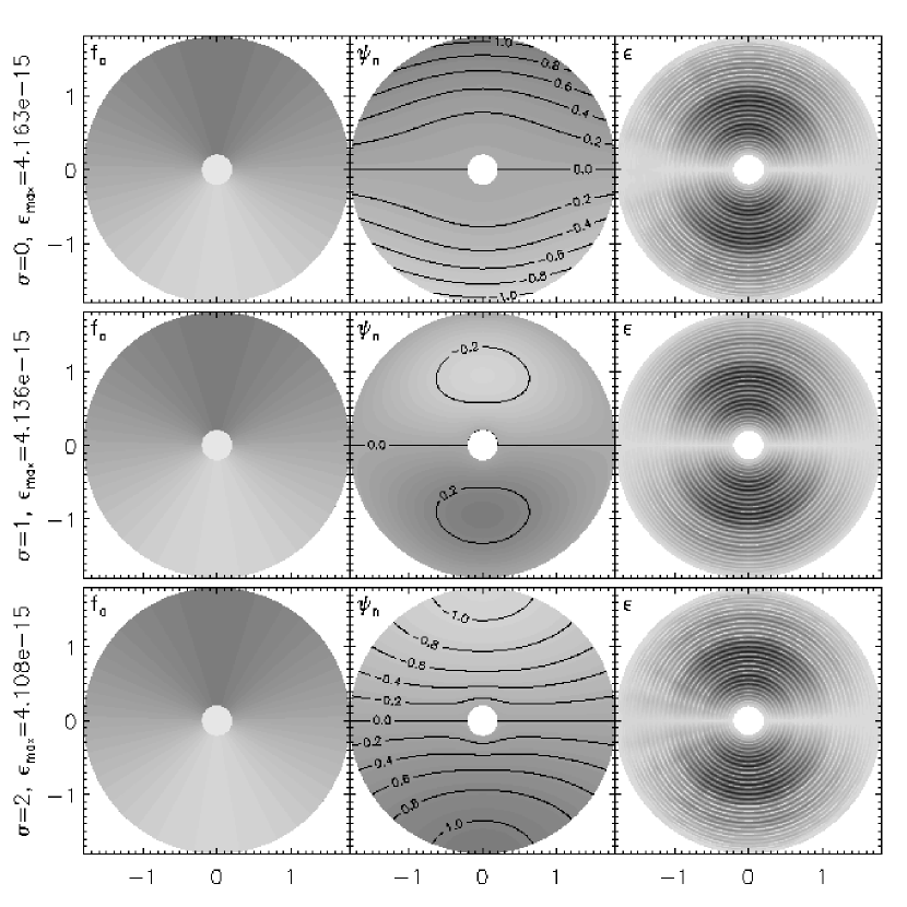
Figure 2.— Grayscale plots of the analytical function $f_{\mathrm{ana}}$, the numerical potential $\psi_{\mathrm{n}}$, and the difference $\epsilon$ between the numerical solution and the analytical solution for the test problem discussed in §4.1. In all plots, darker shades correspond to larger magnitude.

The simplest way to test the Poisson solver is to compare some numerical potential $\psi_{\mathrm{num}}$ obtained by the Poisson solver to its analytical expression $\psi_{\mathrm{ana}}$. The tests in this subsection are done in the computational domain $\mathcal{D}^{(2)}=[0.2,1.8]\times[-\pi,\pi)$. We consider a very simple potential

$$\psi_{\mathrm{ana}}(r,\phi)=\frac{1}{3}\left[r^{2}-\sigma\left(1.82r-\frac{0.0648}{r}\right)\right]\sin\phi,$$ (52)

where $\sigma$ is some arbitrary parameter. We chose this potential because its Laplacian takes the form

$$f_{\mathrm{ana}}(r,\phi)=\nabla^{2}\psi_{\mathrm{ana}}=\sin\phi,$$ (53)

which is independent of $\sigma$. Hence, the parameter $\sigma$ forces our solution to satisfy different boundary conditions.

We choose three different boundary conditions to test the Poisson solver. The first one is

$$\left\{\begin{array}[]{rcl}\psi_{\mathrm{ana}}(r_{\min},\phi)&=&\frac{1}{3}r_{\min}^{2}\sin\phi\\ \psi_{\mathrm{ana}}(r_{\max},\phi)&=&\frac{1}{3}r_{\max}^{2}\sin\phi\end{array}\right.\;,$$ (54)

which corresponds to $\sigma=0$. For the second one, we choose the vanishing boundary condition

$$\left\{\begin{array}[]{rcl}\psi_{\mathrm{ana}}(r_{\min},\phi)&=&0\\ \psi_{\mathrm{ana}}(r_{\max},\phi)&=&0\end{array}\right.\;,$$ (55)

which corresponds to $\sigma=1$. Finally, we also choose

$$\left\{\begin{array}[]{rcl}\psi_{\mathrm{ana}}(r_{\min},\phi)&=&\frac{1}{3}(r_{\min}^{2}-3.64r_{\min}+0.1296/r_{\min})\sin\phi\\ \psi_{\mathrm{ana}}(r_{\max},\phi)&=&\frac{1}{3}(r_{\max}^{2}-3.64r_{\max}+0.1296/r_{\max})\sin\phi\end{array}\right.\;,$$ (56)

which corresponds to $\sigma=2$. In Figure 2, we show the contour of $f_{\mathrm{ana}}$, $\psi_{\mathrm{num}}$, and the difference, $\epsilon=|\psi_{\mathrm{num}}-\psi_{\mathrm{ana}}|$, for each choice of $\sigma$. The contour lines for $\psi_{\mathrm{num}}$ show clearly how the boundary conditions change the solution. The numerical results agree very well with the analytical solution and the difference is only of order $10^{-15}$, which is the machine accuracy.

4.2. Time Independent Tests of Gravity Integrator

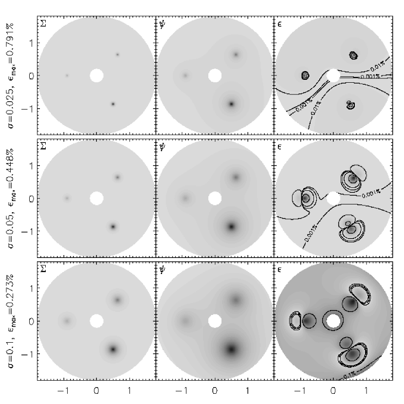
Figure 3.— Grayscale plots of the density $\Sigma$, the potential $\psi$, and the difference $\epsilon$ between the analytical and the numerical values of the gravitational potential for a selection of infinitesimally thin exponential disks (§4.2). The top panel corresponds to $\sigma=0.025$, the middle panel corresponds to $\sigma=0.05$, and the bottom panel corresponds to $\sigma=0.1$.

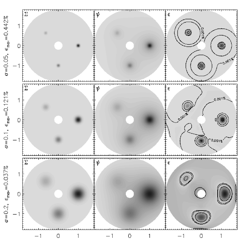
Figure 4.— Grayscale plots of the density $\Sigma$, the potential $\psi$, and the difference $\epsilon$ between the analytical and the numerical value of the gravitational potential of a collection of three-dimensional Gaussian spheres (§4.2). The top panel corresponds to $\sigma=0.05$, the middle panel corresponds to $\sigma=0.1$, and the bottom panel corresponds to $\sigma=0.2$.

To test the gravity integrator, we consider an infinitesimally thin disk, with an exponentially decaying surface density, i.e.,

$$\rho(r,\phi,z)=\Sigma(r,\phi)\delta(z)=\Sigma_{0}e^{-r/\sigma}\delta(z).$$ (57)

The corresponding potential on the $z=0$ plane is given by

$$\psi(r,\phi)=-\pi G\Sigma_{0}r[I_{0}(y)K_{1}(y)-I_{1}(y)K_{0}(y)]$$ (58)

where $y\equiv r/2\sigma$ (Binney & Tremaine, 1987). The functions $I_{n}(y)$ and $K_{n}(y)$ are the modified Bessel functions of the first and second kinds, respectively. The modified Green’s function for this problem is simply

$$\mathcal{G}(r,\phi,r^{\prime},\phi^{\prime})=\frac{-G}{\sqrt{r^{2}+r^{\prime 2}-2rr^{\prime}\cos(\phi-\phi^{\prime})}}.$$ (59)

In order to test our gravity integrator for non-axisymmetric problems, we place three disks in the computational domain with each disk centered at some $(r_{i},\phi_{i})$. Let

$$R_{i}\equiv\sqrt{r^{2}+r_{i}^{2}-2rr_{i}\cos(\phi-\phi_{i})}$$ (60)

be the distance between $(r_{i},\phi_{i})$ and $(r,\phi)$. Normalizing the total mass for each disk to unity, we have

$$\Sigma_{(r_{i},\phi_{i})}(r,\phi)=\frac{1}{2\pi\sigma^{2}}\exp\left(-\frac{R_{i}}{\sigma}\right).$$ (61)

The corresponding potential is

$$\psi_{(r_{i},\phi_{i})}(r,\phi)=-\frac{G}{\sigma}y_{i}[I_{0}(y_{i})K_{1}(y_{i})-I_{1}(y_{i})K_{0}(y_{i})]\;,$$ (62)

where $y_{i}\equiv R_{i}/2\sigma$.

Because the potential is singular, we put the center of each disk off grid. Specifically, we choose the coordinates $(0.9,\pi/4)$, $(0.9,\pi)$, and $(1,-\pi/3)$. We also change the total mass of each disk, in order to avoid cancellation of errors by symmetry, by multiplying them by different constants so that

$$\Sigma_{\mathrm{ana}}(r,\phi)=\Sigma_{(0.9,\pi/4)}(r,\phi)+\frac{1}{2}\Sigma_{(0.9,\pi)}(r,\phi)+2\Sigma_{(1,-\pi/3)}(r,\phi).$$ (63)

We repeated this test for different choices of $\sigma$, namely, $\sigma=0.025$, $\sigma=0.05$, and $\sigma=0.1$. In Figure 3, we show the grayscale plots for $\Sigma_{\mathrm{ana}}$, $\psi_{\mathrm{num}}$, and the fractional error $\epsilon=|\psi_{\mathrm{num}}/\psi_{\mathrm{ana}}-1|$, for each value of $\sigma$. The contour lines in the error plots show that, at the smooth density region, the error is of order $10^{-5}$. The maximum errors appear around the density peak, where the analytic potential is singular.

Besides being able to handle a $\delta$-function in the $z-$direction, our gravity integrator is able to solve problems with other time-independent and $\phi$-independent vertical structures. For example, we consider the Gaussian sphere given by

$$\rho(r,\phi,z)=\frac{M}{(2\pi\sigma^{2})^{3/2}}\exp\left[-\frac{r^{2}+z^{2}}{2\sigma^{2}}\right]\;,$$ (64)

which is normalized so that the total mass is $M$. Here $\sigma$ is a parameter that controls the spread of the mass in each sphere. As $\sigma\rightarrow 0$, the Gaussian sphere approaches a point source. If we have a collection of such spheres with the same $\sigma$, the vertical structure can be factored out of the equations.

Using Gauss’ law, we find that the potential on the $z=0$ plane is given by

$$\psi(r,\phi)=-\frac{1}{r}\mathrm{erf}\left(\frac{r}{\sqrt{2}\sigma}\right)\;,$$ (65)

where $\mathrm{erf}(x)$ is the error function

$$\mathrm{erf}(x)=\frac{2}{\sqrt{\pi}}\int_{0}^{x}e^{-x^{\prime 2}}dx^{\prime}.$$ (66)

For a collection of Gaussian spheres centered on the $z=0$ plane with the same $\sigma$, we can factor out the $z$-dependence, i.e.

$$\rho(r,\phi,z)=\sum_{i}\rho_{(r_{i},\phi_{i})}(r,\phi,z)=Z(r,z)\sum_{i}\Sigma_{(r_{i},\phi_{i})}(r,\phi)\;,$$ (67)

where we have used the same notation as in the previous subsection to indicate that the center of each sphere is located at $(r_{i},\phi_{i})$. The normalized vertical structure is given by

$$Z(r,z)=\frac{1}{\sqrt{2\pi\sigma^{2}}}\exp\left(-\frac{z^{2}}{2\sigma^{2}}\right).$$ (68)

The surface density for each Gaussian sphere is, therefore,

$$\Sigma_{(r_{i},\phi_{i})}(r,\phi)=\frac{1}{2\pi\sigma^{2}}\exp\left(-\frac{R_{i}^{2}}{2\sigma^{2}}\right),$$ (69)

where $R_{i}$ is defined in equation (60).

The modified Green’s function for our problem is

$$\mathcal{G}(r,\phi;r^{\prime},\phi^{\prime}) = \int_{-\infty}^{\infty}\frac{-Z(r^{\prime},z^{\prime})dz^{\prime}}{\sqrt{r^{2}+r^{\prime 2}-2rr^{\prime}\cos(\phi-\phi^{\prime})+z^{\prime 2}}}$$ (70)

$$= -\frac{e^{R^{2}/4}K_{0}(R^{2}/4)}{\sqrt{2\pi\sigma^{2}}}\;,$$

where $K_{0}$ denotes the modified Bessel function of the second kind and we have set $G=1$ for simplicity. We use the modified Green’s function described in equation (70) to obtain the corresponding $\check{\mathcal{I}}_{nm}(r_{k})$. Then we follow the algorithm described in §3.2 to perform the calculation for the gravitational field for three Gaussian spheres located at $(r,\phi)=(1,0)$, $(0.75,2\pi/3)$, and $(1.25,-2\pi/3)$ with a total mass of $2$, $1/2$, and $1$, respectively, i.e.,

$$\Sigma_{\mathrm{ana}}(r,\phi)=2\Sigma_{(1,0)}(r,\phi)+\frac{1}{2}\Sigma_{(0.9,3\pi/4)}(r,\phi)+\Sigma_{(1,-\pi/2)}(r,\phi)$$ (71)

In Figure 4, we show the numerical solutions for $\sigma=0.05$, $\sigma=0.1$, and $\sigma=0.2$. The maximum numerical error is less than $0.5\%$.

4.3. Free Fall of a Dust Ring Under Self-Gravity

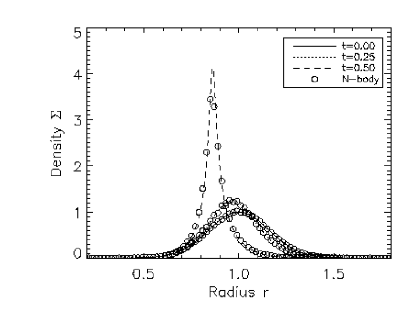
Figure 5.— The radial density profile of the numerical solution for a free-falling dust ring at $\phi=0$. The solid lines represent the solution using our spectral algorithm and the open circles represent the solution using a simple N-body code.

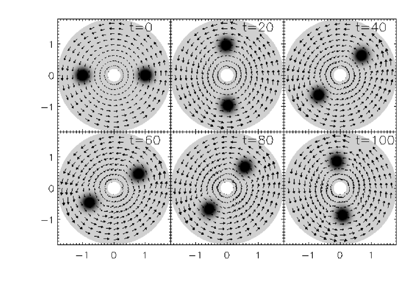
Figure 6.— Grayscale plots of the density $\Sigma$ of the two orbiting cylinders and vectors plots of the velocity fields at different times in the simulation. In all plots, darker colors correspond to larger magnitudes.

In order to perform a dynamic test of our spectral self-gravity solver, we follow the free-fall of a self-gravitating dust ring. The initial condition of this problem is the same as in §4.1 of Chan et al. (2005), i.e.,

$$\rho(r,\phi,z)=\rho(r,\phi)=\exp[-20(r-1)^{2}],$$ (72)

and the initial velocity is zero. The only difference is that, this time, we explicitly calculate the self-gravity of the flow instead of using the gravitational field provided by a central object. We set the gravitational constant to $G=1$ and let the ring free fall. We neglect pressure and viscosity and set the resolution to $513\times 64$ in order to resolve the sharp peak in the density profile that appears at late times.

In order to test our implementation of the spectral method and in the absence of an analytic solution to the problem we wrote a very simple N-body algorithm. We placed 100,000 particles in the computational domain based on the initial density of the ring. Then we computed the gravitational interactions between each particle pair directly and integrated their trajectories.

In Figure 5, we plot the density profiles of the numerical solution of the free falling dust ring at $\phi=0$ using the spectral algorithm and the N-body method. Different lines represent the solution from our pseudo-spectral algorithm at different times and the open circles represent the solution from the particle method. The two solutions agree very well.

4.4. Orbiting Cylinders

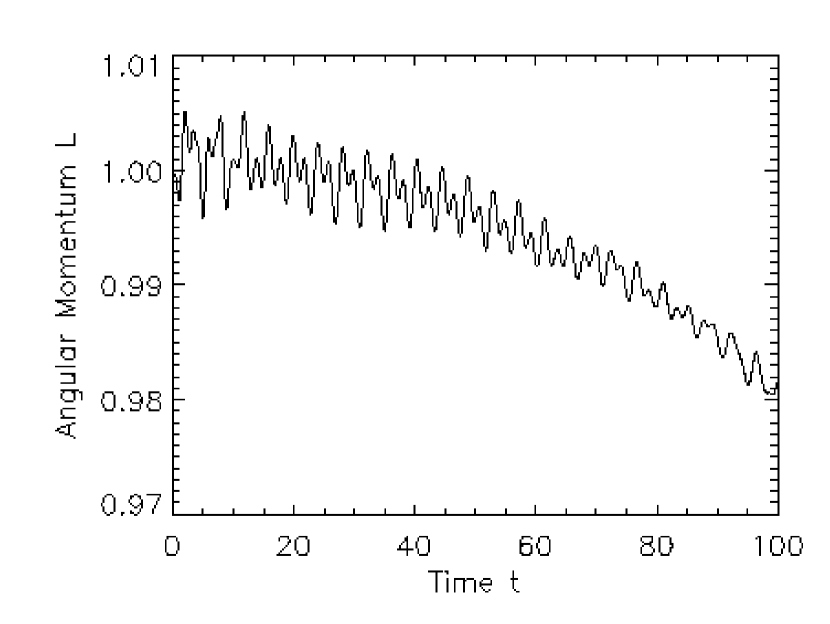
Figure 7.— The total angular momentum of the orbiting cylinders (normalized initially to unity) as function of time. The angular momentum is conserved to better than 2% over $t=100$, which corresponds to about 16 periods or $\sim 5\times 10^{4}$ timesteps.

We adopt this test from Fryer et al. (2005), who simulated two spheres orbiting around each other with smooth particle hydrodynamics. Because our algorithm is two-dimensional, we assume that all variable are independent of $z$ and modify the problem to two infinite cylinders orbiting around each other.

Because the region outside the cylinders has very low density, small fluctuations of the solution in this low-density region result in a large error in the pressure force. In order to resolve the numerical instability that arises from this effect, we evolve the whole set of hydrodynamic equations including the energy equation and introduce a small background term in both the continuity equation and the energy equation. This background needs to be small compared to the physical properties of the cylinders so that it does not affect the orbital motion significantly, while at the same time it needs to be large enough so it can screen out the errors at the low density region in our algorithm. Then, a strong spectral filter is applied to the velocity field to reduce numerical instabilities. The spectral filters for density and energy, on the other hand, are relatively weak in order to conserve mass and total energy.

We consider a Gaussian density distribution for each cylinder

$$\Sigma(r,\phi)=\frac{e^{-r^{2}/2\sigma^{2}}}{2\pi\sigma^{2}}.$$ (73)

In order to find the initial condition for the energy equation, we first need to solve for the gravitational potential using the Neumann boundary condition $\partial\psi/\partial r=0$ at the origin. The second boundary condition is not important here because it only shifts the potential by a constant, which does not affect the gravitational field. Setting the arbitrary constant for the second boundary condition to zero, we obtain

$$\psi=G\left[2\ln r-\mathrm{Ei}\left(-\frac{r^{2}}{2\sigma^{2}}\right)\right],$$ (74)

where $\mathrm{Ei}(x)$ is the exponential integral function defined by

$$\mathrm{Ei}(x)=-\int_{x}^{\infty}\frac{e^{-x}}{x^{\prime}}dx^{\prime}\;.$$ (75)

The corresponding gravitational field of this potential is

$$g(r,\phi)=\frac{2G}{r}\left(e^{-r^{2}/2\sigma^{2}}-1\right).$$ (76)

Therefore, we require the pressure to be

$$P(r,\phi)\equiv\int\Sigma g\;dr=\frac{G}{2\pi\sigma^{2}}\left[\mathrm{Ei}(-r^{2}/\sigma^{2})-\mathrm{Ei}(-r^{2}/2\sigma^{2})\right]$$ (77)

in order to balance self-gravity. Note that we again set the integration constant to zero in the pressure. The modified Green’s function for this problem is

$$\mathcal{G}(r,\phi,r^{\prime},\phi^{\prime})=G\ln\left[r^{2}+r^{\prime 2}-2rr^{\prime}\cos(\phi-\phi^{\prime})\right]\;.$$ (78)

In our simulation we have two Gaussian cylinders centered at $(r_{i},\phi_{i})$. Therefore, we set

$$\Sigma_{(r_{i},\phi_{i})}(r,\phi)=\frac{e^{-R_{i}^{2}/2\sigma^{2}}}{2\pi\sigma^{2}}$$ (79)

and

$$P_{(r_{i},\phi_{i})}(r,\phi)=\frac{G}{2\pi\sigma^{2}}\left[\mathrm{Ei}(-R_{i}^{2}/\sigma^{2})-\mathrm{Ei}(-R_{i}^{2}/2\sigma^{2})\right],$$ (80)

where $R_{i}$ is defined in equation (60). Because the pressure is singular when $R_{i}=0$, we choose the initial position of the cylinders $(r_{i},\phi_{i})$ off grid. In particular, we also choose the background density such that the area between the cylinders contains only $1\%$ of the total mass in the whole system. Because the area of our domain is $\pi(1.8^{2}-0.2^{2})=3.2\pi$, we set

$$\Sigma(r,\phi)=0.99\left[\Sigma_{(1,10^{-3})}(r,\phi)+\Sigma_{(1,\pi+10^{-3})}(r,\phi)\right]+\frac{0.02}{3.2\pi}$$ (81)

and

$$P(r,\phi)=P_{(1,10^{-3})}(r,\phi)+P_{(1,\pi+10^{-3})}(r,\phi)+\frac{0.02}{3.2\pi}.$$ (82)

The initial energy is then chosen using the equation $E=3P/2$ that is based on an ideal gas law. Setting $G=1$, the angular velocity of the cylinder needed to balance the gravitational force is equal to unity. Hence, we set the initial velocities to

$$v_{r}=0,\ \ \ v_{\phi}=r.$$ (83)

We use $\sigma=0.1$ and evolve the simulation to a dimensionless time $t=100$, which is equal to about 16 complete orbital rotations. In Figure 6, we show the gray-scale plots of the density as well as the velocity field for different times in the simulation. In Figure 7, we plot the angular momentum as a function of time. Our algorithm is able to conserve angular momentum to better than 2% for up to about 16 complete orbiting motion, which corresponds to $\sim 5\times 10^{4}$ timesteps. The 2% dissipation of angular momentum is mostly due to the strong spectral filtering, which is equivalent to artificial viscosity, and the deformation of the two cylinders during the simulation.

5. The Stability of Self-Gravitating Hydrodynamic Disks

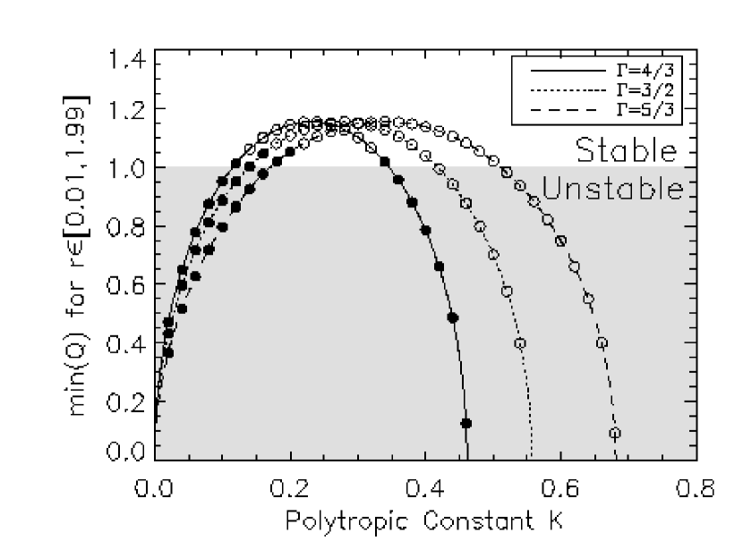
Figure 8.— The minimum value of the Toomre parameter $\min(Q)$ anywhere in the disk, for different values of the polytropic constant $K$. The three different lines correspond to different values of the polytropic index $\Gamma$. When $\min(Q)<1$, i.e. in the shaded region, the linear analysis suggests that the disk is unstable. Filled circles denote simulations in which the disk was unstable, whereas open circles denote simulations in which the disk was stable.

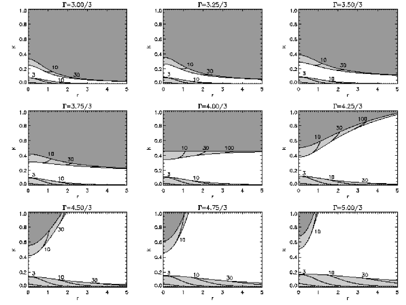
Figure 9.— The Toomre parameter $Q^{2}$ as a function of radius $r$ for solutions with different values of the polytropic constant $K$. The dark gray region corresponds to $Q^{2}<0$, for which no steady-state rotating solution exists; the light gray region corresponds to $0<Q^{2}<1$ which is Toomre unstable; the white region corresponds to $Q^{2}>1$, which is Toomre stable. The contour lines correspond to the size of the minimum unstable wavelength according to the linear mode analysis.

Pseudo-spectral methods effectively evolve in time the hydrodynamic equations for each mode independently. For this reason, they are ideal tools for confirming the results of linear mode analysis and for extending them to the non-linear regime. As a case study, we address here numerically the stability of self-gravitating infinitesimally-thin disks.

We consider self-gravitating gas disks with a polytropic equation of state

$$P=K\Sigma^{\Gamma},$$ (84)

where $K$ is the polytropic constant and $\Gamma$ is the polytropic index. The disks are locally stable to all non-axisymmetric perturbations (Goldreich & Lynden-Bell, 1965a, b; Julian & Toomre, 1966). For axisymmetric perturbations, linear-mode analysis of the hydrodynamic equations results in the dispersion relation (Binney & Tremaine, 1987)

$$\omega^{2}=\kappa^{2}-2\pi G\Sigma|k|+k^{2}c_{\mathrm{s}}^{2},$$ (85)

where we use $c_{\mathrm{s}}$ to denote the sound speed of the gas, $\kappa$ to denote the epicyclic frequency in the disk, and $\omega$ and $k$ to denote the mode frequency and wavenumber, respectively. The disk is locally stable if $\omega^{2}>0$. The condition for all modes to be stable is given by Toomre’s stability criterion (Safronov, 1960; Toomre, 1964),

$$Q\equiv\frac{c_{\mathrm{s}}\kappa}{\pi G\Sigma}>1\;.$$ (86)

Although criterion (86) is only a local condition, it is also sufficient for global stability of axisymmetric modes with $kr\gg 1$. At the critical value $Q=1$, the disk can be globally unstable to non-axisymmetric modes. As $Q$ increases, the disk becomes globally stable to all non-axisymmetric modes. However, for very large values of $Q$, pressure dominates the self-gravity effects and the disk becomes globally unstable to non-axisymmetric perturbations again. Our goal in this section is to study numerically the stability of self-gravitating disks in situations where the unstable wavelengths are larger than the characteristic length scales in the disks.

We simulate the time evolution of disks that obey Plummer’s density model (see Binney & Tremaine, 1987, chapter 2)

$$\Sigma(r)=\frac{M_{\mathrm{d}}\sigma}{2\pi(r^{2}+\sigma^{2})^{3/2}}\;,$$ (87)

where $M_{\mathrm{d}}$ stands for the initial disk mass and $\sigma$ is a parameter that controls the central concentration of the disk density. The corresponding gravitational potential (at the $z=0$ plane) is given by

$$\psi(r)=-\frac{GM_{\mathrm{d}}}{\sqrt{r^{2}+\sigma^{2}}}.$$ (88)

We set the initial radial velocities to zero, i.e., $v_{r}=0$, and choose the azimuthal velocities, $v_{\phi}$, so as to balance the pressure and self-gravity of the flow, i.e.,

$$\frac{v_{\phi}^{2}}{r}=\frac{2\pi G\Sigma r}{\sigma}-\frac{3K\Gamma\Sigma^{\Gamma-1}r}{r^{2}+\sigma^{2}}.$$ (89)

Although Plummer’s model assumes that the density is a $\delta$-function along the $z$-direction, its corresponding scale height $H=rc_{\mathrm{s}}/v_{\phi}$ is given by

$$\frac{H}{r}=\frac{c_{\mathrm{s}}}{v_{\phi}}=\left(\frac{2\pi Gr^{2}}{K\Gamma\Sigma^{\Gamma-2}\sigma}-\frac{3r^{2}}{r^{2}+\sigma^{2}}\right)^{-1/2}.$$ (90)

We choose $129\times 64$ grid points and perform the simulations in the domain $[0.005,5]\times[-\pi,\pi)$ with $\sigma=1$. We set the total disk mass to $M_{\mathrm{d}}=1$.

Figure 8 a parameter study of the dependence of the stability of the disk on the polytropic index $\Gamma$ and the constant $K$. We plot the minimum value of the Toomre parameter $\min(Q)$ anywhere in the disk against $K$. The three different lines correspond to different values of the polytropic index $\Gamma$. According to linear analysis, when $\min(Q)<1$, there is some region in the disk where the disk becomes unstable. We present the results of our simulation on the same plot, with filled circles denoting the solutions that become unstable and with open circles the solutions that remained stable during the course of the simulations.

For small values of the polytropic index ($\Gamma\leq 4/3$) or for small values of the polytropic constant ($K<0.2$), our numerical simulations agree with the predictions of the linear mode analysis. The small disagreements near the $Q=1$ separatrix come from two facts: that, (i) we have a finite domain of integration on which we have to impose boundary conditions, and (ii) we cannot calculate the evolution of the instabilities and the perturbations in the gravitational field from matter outside the boundaries. Regarding point (i), we have used the absorbing boundary condition discussed in the first paper in the series (see Chan et al., 2005), which reduce the reflection significantly. However, a very small but finite amount of the energy of the wave is still trapped in the domain, which causes the instability. As a result, when the gravitational potential deviates from Plummer’s model because of the finite size of the domain, the disk close to the outer boundaries becomes unstable.

A striking difference, however, appears when the polytropic index and the polytropic constant become larger: our numerical solutions are always stable, contrary to the predictions of the linear mode analysis. The reason for this disagreement between the linear mode analysis and our numerical simulations becomes evident in Figure 9, where we plot Toomre’s parameter $Q^{2}$ as function of radius $r$ for different values of the polytropic constant $K$. When $Q^{2}<0$, there is no initial value of the azimuthal velocity $v_{\phi}$ that satisfies the steady-state equation for radial force balance; we shade this region using dark gray. For $0<Q^{2}<1$, the disk is unstable according to Toomre’s criterion; we shade this region using light gray. Finally, when $Q^{2}>1$ the disk is linearly stable; we leave this region white. We also plot in Figure 9 contours that correspond to the minimum unstable wavelength, in the unstable region, computed by

$$\frac{2\pi}{\lambda_{\min}}=k_{\max}=\frac{\pi\Sigma}{c_{\mathrm{s}}}\left(1+\sqrt{1-Q^{2}}\right)$$ (91)

Figure 9 shows that when $\Gamma>4/3$ and for large values of the polytropic constant $K$, the minimum unstable wavelength is larger than the extent of the region in which the disk is unstable. For example, for $\Gamma=4.5/3$ and for $K\in[0.42,0.56]$, the unstable region only extends to $r\in[0,1.5]$. However, in that same region, the minimum unstable wavelength is $\lambda_{\min}\approx 3$, in the appropriate units. Because the unstable wavelengths are larger than the characteristic length scale in the system (which can be defined here as the extent of the region in which $0<Q<1$), the approximations involved in the linear mode analysis are not justified. Indeed, the numerical simulations show that the unstable modes cannot grow and the disk is stable.

6. Conclusions

Problems that involve self-gravity are usually time-consuming tasks in computational physics. In standard finite difference methods, Poisson’s equation is solved as the steady state of a diffusion equation (using relaxation and over-relaxation methods) and has to be recalculated together with the hydrodynamic equations at every timestep. Although hybrid algorithms have been developed which use high-order methods to solve Poisson’s equation, finite difference schemes are still used for evolving the hydrodynamic equations. The resulting inconsistency in the order of differencing the hydrodynamic equations and Poisson’s equations either significantly reduces the accuracy of the Poisson solver, or requires the extra complication of interpolating the gravitational filed at each grid point. More importantly, existing two-dimensional hybrid algorithms can only address a limited number of self-gravitating problems because the solutions to the two-dimensional and three-dimensional Poisson’s equation are fundamentally different (see §1 and §2).

In this paper, we presented two different approaches to using pseudo-spectral methods to solve self-gravity problems. For the first approach, we described the implementation of a standard pseudo-spectral Poisson solver that solves the two-dimensional Poisson’s equations to machine accuracy. Instead of solving a diffusion equation, spectral methods allowed us to invert the Poisson operator in spectral space, making the algorithm fast and accurate. For the second approach, we investigated a fast gravity integrator for disks-like flows with known, time-independent vertical structures. This algorithm allowed us to study the evolution of flows with finite, but not only infinitesimal, thickness. This improvement allows two-dimensional algorithms to solve a whole new class of problems. We demonstrated here the ability of our algorithm to compute properly and efficiently the gravitational potential of flattened flows using different test problems. Even for the high resolution that corresponds to $129\times 256$ collocation points, our Poisson solvers and integrator use less than 10% of the total computational time.

We also explored how to extend Toomre’s stability criterion to self-gravitating disks for which the characteristic properties of the flows change over a length scale that is shorter than the minimum unstable wavelength. Based on our simulations, we find that for Plummer’s density model, if the disk is hot and has a polytropic index $\Gamma>4/3$, all oscillatory modes in the disk are stable, contrary to the predictions of the analytic calculation.

References

- Baltensperger & Trummer (2003) Baltensperger, R., & Trummer, M.R. 2003, SIAM J. Sci. Comput., 24, 1465
- Balbus & Papaloizou (1999) Balbus, S.A., & Papaloizou, J.C.B. 1999, ApJ, 521, 650
- Bertin (1997) Bertin, G. 2001, ApJ, 478, L71
- Bertin & Lodato (1999) Bertin, G., & Lodato, G. 1999, å, 350, 694
- Bertin & Lodato (2001) Bertin, G., & Lodato, G. 2001, å, 370, 342
- Binney & Tremaine (1987) Binney, J., & Tremaine, S. 1987, Galactic Dynamics (Princeton: Princeton University Press)
- Boss & Myhill (1992) Boss, A.P., & Myhill, E.A. 1992, ApJS, 83, 331
- Boss (1998) Boss, A.P. 1998, ApJ, 503, 923
- Broderick & Rathore (2004) Broderick, A. E., & Rathore, Y. 2004, astro-ph/0411652
- Chan et al. (2005) Chan, C.-K., Psaltis, D., & Ozel, F. 2005, ApJ, 628, XXX
- Cohl & Tohline (1999) Cohl, H.S., & Tohline, J.E. 1999, ApJ, 527, 86
- Dimmelmeier et al. (2005) Dimmelmeier, H., Novak, J., Font, J. A., Ibáñez, J. M., Müller, E. 2005, Phys. Rev. D, 71, 4023
- Frank et al. (2002) Frank, J., King, A., & Raine, D. 2002, Accretion Power in Astrophysics (Cambridge: Cambridge Univ. Press)
- Fryer et al. (2005) Fryer, C., Rockefeller, G., & Warren, M.S. 2005, ApJ, submitted
- Frigo & Johnson (2003) Frigo, M., & Johnson, S.T. 2003, FFTW User Manual (Avalible online at http://www.fftw.org/fftw3_doc/)
- Grandclement et al. (2001) Grandclement, P., Bonazzola, S., Gourgoulhon, E., Marck, J.-A. 2001, J. Comp. Phys, 170, 231
- Goldreich & Lynden-Bell (1965a) Goldreich, P., & Lynden-Bell, D. 1965, MNRAS, 130, 97
- Goldreich & Lynden-Bell (1965b) ———. 1965, MNRAS, 130, 125
- Julian & Toomre (1966) Julian, W.H., Toomre, A. 1996, ApJ, 146, 810
- Mejía et al. (2005) Mejía, A.C., Durisen, R.H., Pickett, B.K., Cai, K. 2005, ApJ, 619, 1098
- Myhill & Boss (1993) Myhill, E.A., & Boss, A.P. 1993, ApJS, 89, 345
- Pickett et al. (1998) Pickett, B.K., Cassen, P., Durisen, R.H., & Link, R. 1998, ApJ, 504, 468
- Pickett et al. (2000) ———. 2000, ApJ, 529, 1034
- Pickett et al. (2003) Pickett, B.K., Mejía, A.C., Durisen, R.H., Cassen, P.M., Berry, D.K., Link, R.P. 2003, ApJ, 590, 1060
- Safronov (1960) Safronov, V.S. 1960, AnAp, 23, 979
- Stone & Norman (1992) Stone, J.M., & Norman, M.L. 1992, ApJ, 80, 753
- Toomre (1964) Toomre, A. 1964, ApJ, 139, 1217
- Trefethen (2000) Trefethen, L.N. 2000, Spectral Methods in MATLAB (Philadelphia: SIAM)
- van der Klis (2000) van der Klis, M. 2000, ARA&A, 38, 717