On the Origin of [OII] Emission in Red Sequence and Post-starburst Galaxies

Abstract

We investigate the emission-line properties of galaxies with red rest-frame colors (compared to the $g-r$ color bimodality) using spectra from Data Release 4 of the Sloan Digital Sky Survey (SDSS). Emission lines are detected in more than half of the red galaxies. We focus on the relationship between two emission lines commonly used as star formation rate indicators: H$\alpha$ and [O II] $\lambda$3727. Since [O II] is the principal proxy for H$\alpha$ at $z\sim 1$, the correlation between them is critical for comparison between low-z and high-z galaxy surveys. We find a strong bimodality in [O II]/H$\alpha$ ratio in the SDSS sample, which closely corresponds to the bimodality in rest-frame color. Based on standard line ratio diagnostics, most (nearly all of the) line-emitting red galaxies have line ratios typical of various types of Active Galactic Nuclei (AGN) — most commonly “low-ionization nuclear emission-line regions” (LINERs), a small fraction of “transition objects” (TOs) and, more rarely, Seyferts. Only $\sim 6\%$ of red galaxies have line ratios resembling star-forming galaxies. A straight line in the [O II]-H$\alpha$ EW diagram separates LINER-like galaxies from other categories, provides an effective classification tool complementary to standard line ratio diagnostics. Quiescent galaxies with no detectable emission lines and those galaxies with LINER-like line ratios combine to form a single, tight red sequence in color-magnitude-concentration space. Other than modest differences in the luminosity range they span, these two classes are only distinguished from each other by line strength. We also find that [O II] equivalent widths in LINER- and AGN-like galaxies can be as large as that in star-forming galaxies. Thus, unless objects with AGN/LINER-like line ratios are excluded, [O II] emission cannot be used directly as a proxy for star formation rate; this is a particular issue for red galaxies. Lack of [O II] emission is generally used to indicate lack of star formation when post-starburst galaxies are selected at high redshift. Our results imply, however, that these samples have been cut on AGN properties as well as star formation, and therefore may provide seriously incomplete sets of post-starburst galaxies. Furthermore, post-starburst galaxies identifed in SDSS by requiring minimal H$\alpha$ equivalent width generally exhibit weak but nonzero line emission with ratios typical of AGNs; few of them show residual star formation. This suggests that most post-starburst galaxies may harbor AGNs/LINERs.

1. Introduction

[O II] $\lambda$3727 emission line is a widely used, empirical star formation rate (SFR) indicator, especially at high redshift when H$\alpha$ moves out of the optical window (e.g., Gallagher et al. 1989; Kennicutt 1992; Cowie et al. 1996, 1997; Ellis 1997; Hammer et al. 1997; Hogg et al. 1998; Rosa-González et al. 2002; Hippelein et al. 2003). Although its luminosity is not directly coupled to the ionizing flux, and it is very sensitive to reddening and metallicity effects, it still can be empirically or theoretically calibrated through comparison with H$\alpha$. A variety of calibrations have been developed (Kennicutt 1992, 1998; Kewley et al. 2004; Mouhcine et al. 2005; Moustakas et al. 2005), enabling SFR estimations from [O II] to a reasonable accuracy for star-forming galaxies.

However, many red, elliptical galaxies at $z\sim 0$ also have significant [O II] and other line emission in their spectra (Caldwell 1984; Phillips et al. 1986). Does [O II] also indicate star formation in these galaxies? It has long been realized that star formation is not the only possible source of [O II] emission in galaxies. Active Galactic Nuclei (AGN - especially LINERs), fast shockwaves, post-AGB stars, and cooling flows might also produce [O II] emission. Thus, before we use [O II] as a universal star formation indicator, we need to know how often and to what degree [O II] emission is contaminated by sources other than star formation, especially in red, elliptical galaxies.

The assumption that [O II] measures star formation has been fundamental to many studies. For instance, the lack of [O II] is often used as a criterion for post-starburst galaxy identification. Post-starburst galaxies, as their name suggests, are galaxies that underwent a strong recent star formation epoch but have stopped forming stars. Their spectra can be modeled by a combination of an old stellar population (similar to that of a K giant star or an early-type galaxy) and a young population which is dominated by A stars (Dressler & Gunn 1983). Therefore, these galaxies are commonly known as ‘K+A’ or ‘E+A’ galaxies. With time, these galaxies will display an early-type galaxy spectrum after all the A stars die out in 1 Gyr. Thus, the study of these galaxies is important for understanding galaxy evolution, given the current uncertainty in how elliptical galaxies form.

The identification of these post-starburst galaxies requires a total lack of emission lines, to be certain that star formation has truly stopped. Most works on post-starbursts (e.g., Dressler & Gunn 1983; Zabludoff et al. 1996; Poggianti et al. 1999; Balogh et al. 1999; Tran et al. 2003; Yang et al. 2004; Blake et al. 2004; Tran et al. 2004) have used [O II] as the marker, either because it is the only emission line diagnostic available at high redshifts or for the sake of facilitating comparisons between low and high redshifts and among different authors. Recently, several groups (Goto et al. 2003; Quintero et al. 2004; Balogh et al. 2005) have employed H$\alpha$ emission as the marker for star formation, rather than [O II], for samples of galaxies from the Sloan Digital Sky Survey (SDSS). Usually, a low equivalent width (EW) threshold on [O II], e.g., 2.5Å, is used as the criterion for non-detection of such emission lines, according to the sensitivity in each survey. This reflects an underlying assumption that any emission line would be coming from starforming regions. If this assumption fails to hold—for instance, if the contribution of [O II] from AGN is significant—the post-starburst sample defined by such a method would be incomplete because AGN would be mistakenly discarded as star-forming galaxies. Thus, using [O II] in post-starburst galaxy studies requires a better understanding of the many origins of [O II] in all types of galaxies.

In many studies of AGNs, the opposite question is asked: what fraction of [O II] emission in AGN spectra comes from star formation? A variety of studies of high-ionization AGN (QSOs and Seyferts) have attempted to separate the contributions from AGN and star formation to line emission. It is of special interest to the understanding of the coevolution of the nuclear black holes and the bulges. Croom et al. (2002) found by measuring the Baldwin effects (Baldwin 1977) that most [O II] emission in QSOs might be from the host galaxies instead of the AGN. Richards et al. (2003) found that dust-reddened QSOs have stronger [O II] emission than normal QSOs. One of the many possible explanations is that the host galaxies of those QSOs with higher extinctions have higher star formation rates. In contrast, studies by Ho (2005) show that in quasar spectra there is very little [O II] emission beyond that expected from the AGN itself, indicating a supressed star formation efficiency in quasar host galaxies.

Unlike the controversy in Type I QSOs, the picture is a little clearer for Seyfert 2s and Type II QSOs. Gu et al. (2006) found that [O III]/H$\beta$ and [O III]/[O II] ratios are lower in those Seyfert 2 galaxies with significant star formation, which indicates that star formation could contribute substantially or even dominate the H$\beta$ and [O II] emission. Consistently, Kim et al. (2006) found that Type II QSOs exhibit significantly enhanced [O II]/[O III] ratios relative to Type I QSOs. Combined with their high [O III] luminosities, the high [O II]/[O III] ratio is best explained by a high level of star formation. However, the problem is far from settled. Although the [O II] emission in QSO spectra could be a combination of two or many origins, we still have no idea of their proportions. In addition, QSO hosts are rare among galaxies. Narrow-line, low-luminosity AGN and LINERs (which may or may not be AGN) are much more abundant. The dominant origin of [O II] emission among these galaxies is still unknown.

A variety of approaches can help to distinguish emission lines having different origins. One commonly used method, which is relatively reliable, is emission-line diagnostics (Baldwin et al. 1981; Veilleux & Osterbrock 1987; Rola et al. 1997; Kauffmann et al. 2003, etc.), as also used by many authors mentioned above in QSO studies. This method is effective in distinguishing the two major origins of emission: star formation versus AGN. We will focus on using this method to investigate the origin of [O II] emission in red galaxies in this paper.

The large SDSS redshift survey provides a perfect sample for such a study. Its wide wavelength coverage covers many emission lines from [O II] to H$\alpha$, from which many line ratio diagnostics can be created. At the same time, moderate resolution still allows reasonable line profile fitting to be conducted, giving good control of errors in the line strength measurement. Finally, its unprecedented huge sample size produces reliable statistics. Previous studies of line ratio diagnostics (e.g., Rola et al. 1997) used much smaller datasets with less uniform sampling.

In this paper, we present the discovery of a bimodality in [O II]/H$\alpha$ ratio among galaxies. One mode is largely associated with star-forming galaxies. Galaxies in the other mode generally have line ratios similar to LINERs, with [O II] emission produced by a mechanism not associated with ordinary star formation. Narrow-line Seyferts and Transition Objects mostly fall in between the two dominant populations, consistent with the picture that both star formation and AGN (or some other source) might contribute substantially to the emission in these objects. The [O II]/H$\alpha$ bimodality we find also has important implications for post-starburst studies.

The paper is structured as follows. In §2, we describe the data used. (The details of our measurement methods are descibed in the Appendices.) In §3, we compare [O II] emission-line strength with H$\alpha$ for all types of galaxies. We demonstrate that red and blue galaxies show different [O II]-H$\alpha$ correlations, which appear to reflect different emission origins. Classification based on this [O II]/H$\alpha$ bimodality are made and investigated later in §4.1 with the standard line ratio diagnostics. Possible origins of the emission in red galaxies are discussed. With the conclusions drawn from that, we show in §5 how the selection of post-starbursts using [O II] leads to an incomplete sample and explore the nature of emission in post-starbursts. We summarize in §6. The cosmology used is a flat $\Lambda$ cold dark matter ($\Lambda$CDM) cosmology with density parameter $\Omega_{m}=0.3$.

2. Overview of Data and Line Measurements

The SDSS (York et al. 2000; Stoughton et al. 2002) is an ongoing imaging and spectroscopic survey that will eventually cover $\sim\pi$ steradians of the celestial sphere. It utilizes a dedicated 2.5-m telescope at Apache Point Observatory. The imaging is done with five broadband filters in drift scan mode ($u,g,r,i,{\rm and}~{}z$; Fukugita et al. 1996; Stoughton et al. 2002). Spectra are obtained with two fiber-fed spectrographs, covering the wavelength range of 3800-9200Å with a resolution of R $\sim 2000$. Fibers have a fixed aperture of 3”.

The spectroscopic data used here have been reduced through the Princeton spectroscopic reduction pipeline (Schlegel et al. in prep), which produces the flux- and wavelength-calibrated spectra. The redshift catalog of galaxies used is from the NYU Value Added Galaxy Catalog (Blanton et al. 2005b, http://wassup.physics.nyu.edu/vagc/). K-corrections were derived using Blanton et al. (2003a)’s kcorrect code v3_2. All the magnitudes used in this paper are K-corrected to a redshift of $z=0.1$ by shifting the SDSS bandpasses to bluer wavelengths by a factor of 1.1 (Blanton et al. 2003b). Thus all magnitudes and color notations carry a superscript or subscript of 0.1 .

The results in this paper are based on the spectra of $\sim 400,000$ galaxies contained in the SDSS Data Release Four (Adelman-McCarthy et al. 2006, DR4). We employ a catalog of objects targeted by the main galaxy survey that have been spectroscopically confirmed as galaxies; QSOs are not included in this sample. Target selection for the main galaxy sample is described in Strauss et al. (2002). The magnitude limit is $r=17.77$ in Petrosian magnitudes after correction for the foreground galactic extinction following Schlegel et al. (1998).

For many plots (Figs. 2, 3, 5, 6, 12, and 13) in this paper, we used a volume-limited sample of about 55,000 galaxies with $0.07<z<0.10$ and $M_{{}^{0.1}r}-5\log h$ brighter than -19.5, and to have well-measured spectra in the vicinity of [O II] and H$\alpha$ (using criteria described in the Appendix B). However, in color-magnitude diagrams and line ratio diagnostic plots (Figs. 1, 4, 7, 8, 9, 11, and 14), a magnitude limited sample with $0.05<z<0.10$ and $r$ brighter than 17.77 is used to cover a wider range in galaxy luminosity and metallicity. The redshift ranges of these samples are chosen for several reasons. First, selecting very nearby galaxies is unfavorable because Sloan spectra are taken with a 3” fiber which only covers a small fraction of each galaxy at low redshifts. Secondly, objects at redshifts greater than $z=0.15$ are disfavored because blue galaxies drop out the $r$-band selected sample quickly with increasing $z$. Additionally, the bad column on the CCD around 7300Å heavily hinders the accurate measurements of H$\alpha$ at $z\sim 0.114$ and other lines at higher $z$. The median S/N of the spectra in the volume-limited sample is 18.5 per pixel.

For each galaxy, we subtract the stellar continuum and measure the emission line fluxes and equivalent widths for [O II] $\lambda$3727, H$\beta$, [O III] $\lambda$5007, [O I] $\lambda$6300, H$\alpha$, and [N II] $\lambda$6583. Zero point errors in the equivalent widths are removed and the corrections are propagated into fluxes. Reliable emission line detections are defined as 3 or more $\sigma$ detection in EW. For the technical details of our stellar continuum subtraction procedure, emission line measurements, and zero point determinations, see Appendix A and B.

3. [O II] $\lambda$3727 vs. H$\alpha$

3.1. Color Bimodality

Figure 1.— Rest-frame color-magnitude diagram for all SDSS galaxies with redshifts between 0.05 and 0.10. The two solid lines indicate the cut we adopt for separating red and blue galaxies. Red galaxies are defined as the points above the upper line, while blue galaxies are below the lower line. We leave a gap in between to eliminate galaxies with potentially ambiguous status. The vertical dashed line indicates the absolute magnitude limit for the volume-limited sample.

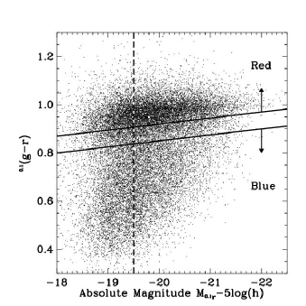
Before diving into line comparisons, we recall that the color distribution of galaxies is highly bimodal, as have been shown repeatedly (e.g., Strateva et al. 2001; Hogg et al. 2002; Blanton et al. 2003b; Baldry et al. 2004; Bell et al. 2004; Weiner et al. 2005; Willmer et al. 2005; Giallongo et al. 2005). Fig. 1 shows the color-magnitude diagram for all SDSS galaxies within $0.05<z<0.10$. We use this sample rather than the volume-limited sample simply to display a wider range in galaxy luminosity.

In color-magnitude space, galaxies fall mainly into two categories. One category is the tight sequence between color and magnitude at the red end (larger value of ${}^{0.1}(g-r)$), commonly called the “red sequence”; the other is the swath of points at bluer colors, which is sometimes referred to as the “blue cloud”. Empirically, blue galaxies mostly have disk-dominated morphologies and are actively forming stars; while red galaxies mostly have bulge-dominated morphologies and are relatively quiescient in terms of star formation.

Although the bimodality is obvious, it is impossible to entirely separate the two populations by color. One possibility is that color provides a poor measurement of some more fundamental property that cleanly distinguishes galaxies into two distinct populations. Alternatively, the absence of a clean separation in color may simply reflect the smooth evolution of one population into the other. It is also likely that both possibilities are involved. For now, we use conservative color cuts to define the samples of red and blue galaxies, as shown with the two solid lines in Fig. 1 and desribed by the following inequalities. We leave a gap in color between the two samples to reduce the importance of color errors and galaxies with ambiguous status. We define these color cuts by:

$${\rm Red:~{}~{}}^{0.1}(g-r) > -0.025(M_{{}^{0.1}r}-5\log h)+0.42$$ (1)

$${\rm Blue:~{}}^{0.1}(g-r) < -0.025(M_{{}^{0.1}r}-5\log h)+0.35.$$ (2)

3.2. [O II]/H$\alpha$ Bimodality

In this paper, we will use both equivalent width (EW) and flux/luminosity measurements of emission lines. For line intensity ratios and SFR measurements, the use of flux is necessary, but fluxes are much more sensitive to dust extinction than equivalent widths. Furthermore, EW will not be affected by imperfect flux calibration. On the other hand, to interpret the EW ratio between two lines, the continuum shape (i.e., the color of the galaxy) needs to be taken into account. In addition, line luminosity and EW describe different sorts of physical quantities: line luminosity describes the total amount of emission, while EW reflects the strength of emission compared to the luminosity of the galaxy. We will primarily employ EW in this paper because it is not subject to variations in galaxy size (in contrast, line luminosity tends to scale with the total luminosity of a galaxy). It is worth noting that the correlations in EW are often tighter than those in luminosity, for all these reasons.

Figure 2.— (a) The distribution of all SDSS galaxies in the volume-limited sample with $0.07<z<0.10$ in H$\alpha$ and [O II] equivalent width for those objects where both lines are detected. There are two [O II]-H$\alpha$ sequences with different slopes. The dashed line indicates an empirical cut (Eq.6) separating the two sequences and is reproduced in following panels. We refer to the population to the left of the line as “High-[O II]/H$\alpha$ galaxies”, and refer to the population to the right as “Low-[O II]/H$\alpha$ galaxies”. (b) Same as panel (a) but in logarithmic space. The shade indicates the number of points per sq. dex. The bimodality in [O II]/H$\alpha$ ratio is even more obvious in this panel. The dashed curve corresponds to the dashed line in panel (a). (c) Same as (b) but only for red galaxies, most of which are on the steep-slope sequence. Shade scale is the same as in panel (b). (d) Same as (b) but only for blue galaxies, most of which are on the shallow-slope sequence. These generally have an [O II]/H$\alpha$ ratio consistent with an origin from star-forming HII regions (see §3.2). Dashed lines in all four panels indicate the same line, which we use throughout this paper to separate the two populations.

Figure 3.— (a) [OII] line luminosity vs. H$\alpha$ line luminosity for all galaxies in the volume-limited sample with $0.07<z<0.1$ detected in both lines. Line luminosities are divided by the SDSS ${}^{0.1}r$- band luminosity to take out the size effect (see §3.2). The same bimodality exists as seen in EW plot. (b) Same as panel (a) but in log-log space. The bimodality clearly stands out. The shade indicates the number of galaxies per sq. dex. The two dashed lines show [O II]/H$\alpha$ ratios of 1.38 and 0.317, corresponding to the median ratio for each of the two modes, respectively. The effect of $A_{V}=2$ of extinction (for $R_{V}=3.1$) is indicated by the arrow, as we do not correct for reddening.

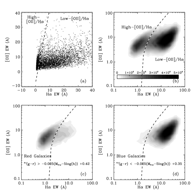
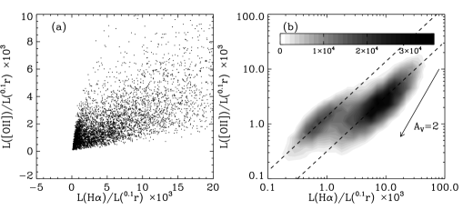
Figure 2 compares [OII] EW with H$\alpha$ EW for galaxies in the volume-limited sample ($0.07<z<0.10$, $M_{0.1r}-5\log h<-19.5$) which have both [O II] and H$\alpha$ positively detected. Clearly, there are two [O II]-H$\alpha$ sequences. One has a shallow slope and extends to very high H$\alpha$ EW. The other sequence has a rather steep slope and very high concentration of points at low H$\alpha$ EW, with [O II] EW spanning a wide range.

The bimodality in the [O II]-H$\alpha$ diagram becomes even more obvious if plotted on a logarithmic scale, as shown in the upper right panel of Fig. 2. Here the shading reflects the density of points in units of number per square dex. The H$\alpha$ EW distribution can be well fit by two log-normal distributions, one centered around 1Å and the other centered around 14Å. In linear space, the high-EW population spans a wide range of EWs, but it becomes much more concentrated in log space.

The bottom two panels in Fig. 2 show [O II] EW vs. H$\alpha$ EW for the red galaxies and blue galaxies separately. The clear difference between the two populations shows immediately that most red galaxies reside on the steep-slope sequence, while most blue galaxies are on the shallow-slope sequence. Clearly, the bimodality in [O II]/H$\alpha$ ratio echoes the color bimodality. Since most blue galaxies are actively forming stars, this is telling us that the shallow-slope sequence must have an [O II]/H$\alpha$ ratio consistent with that produced in HII regions photoionized by O and B stars in star-forming galaxies. What mechanism gives rise to the different ratio seen in red galaxies?

Before addressing this question, we detour briefly to consider another issue. Since we are thus far using equivalent width instead of line luminosity, one might imagine that the bimodality has little to do with emission strength; rather, differences in eqivalent-width ratio might reflect only the different continuum ratios between stellar continua near [O II] and H$\alpha$ in red galaxies versus that of blue galaxies. Since red galaxies have higher continuum ratios of $F_{c}(\mbox{H$\alpha$})/F_{c}(\mbox{[{O~{}II}]})$, they will have a higher value of $\mbox{EW}(\mbox{[{O~{}II}]})/\mbox{EW}(\mbox{H$\alpha$})$ for the same emission line luminosity ratio. This possibility can be checked by comparing L([O II]) to L(H$\alpha$) directly.

As shown by Kennicutt (1990), however, such a plot of luminosity versus luminosity can be quite misleading because of the size effect: for a given class of galaxies, we expect both L([O II]) and L(H$\alpha$) to each have a significant correlation with the stellar mass of the galaxies, especially at the low-mass end, which would veil the true relationship between [O II] and H$\alpha$. This hidden variable can be easily removed by using specific line luminosity; here we divide the line luminosity by the Sloan ${}^{0.1}r$ band luminosity, which is a coarse proxy for the stellar mass. This effectively creates an EW, but one that does not include the continuum color variation between red and blue galaxies. As shown in Fig. 3(a), the same separation between the two sequences persists in a plot of L([O II])/L(${}^{0.1}r$) vs. L(H$\alpha$)/L(${}^{0.1}r$), but with a smaller opening angle between them. The wider opening angle in the equivalent width plot indeed reflects the different continuum ratios between blue and red galaxies, but this is not the whole origin of the bimodality. In panel (b) of Fig. 3, we plot L([O II])/L(${}^{0.1}r$) vs. L(H$\alpha$)/L(${}^{0.1}r$) in logarithmic scale, analogous to the upper right panel in Fig. 2. The bimodality in [O II]/H$\alpha$ ratio again stands out clearly. We omit the plots for subsamples separated in color, due to their close resemblance to the bottom panels of Fig. 2.

Since the continuum ratios are not responsible for the [O II]/H$\alpha$ ratio bimodality, the question of the source of line emission in red galaxies persists. Can the difference between line ratios for blue and red galaxies in [O II]/H$\alpha$ ratio arise from reddening or metallicity dependences for star-forming regions? We investigated this possibility using the SFR(H$\alpha$) and SFR([O II]) calibrations derived by Kennicutt (1998) and Kewley et al. (2004), which explicitly take into account extinction and metallicity corrections:

$${\rm SFR}(\mbox{H$\alpha$}) = 7.9\times 10^{-42}L(\mbox{H$\alpha$}/{\rm ergs^{-1}})M_{\odot}yr^{-1}$$ (3)

and

$${\rm SFR}(\mbox{[{O~{}II}]}) = {7.9\times 10^{-42}L(\mbox{[{O~{}II}]}/{\rm ergs^{-1}})\over 16.73-1.75[\log({\rm O/H})+12]}M_{\odot}yr^{-1}.$$ (4)

By identifying SFR(H$\alpha$) with SFR([O II]), we get

$$L(\mbox{[{O~{}II}]})/L(\mbox{H$\alpha$})=16.73-1.75[\log({\rm O/H})+12].$$ (5)

First, we can check that the [O II]/H$\alpha$ ratio seen among blue galaxies is consistent with that produced in star-forming HII regions. The galaxies to the right and below the demarcation in Fig. 2 have a median [O II]/H$\alpha$ flux ratio of 0.317, as indicated by the lower dashed line in Fig. 3b. Their median H$\alpha$/H$\beta$ ratio (the Balmer decrement) is 4.75. This corresponds to a median extinction $A_{V}$ of 1.60 (assuming $R_{V}=A_{V}/E(B-V)=3.1$ and an intrinsic H$\alpha$/H$\beta$ ratio of 2.85 for case B recombination at $T=10^{4}{\rm K}$ and $n_{e}\sim 10^{2}-10^{4}cm^{-3}$ (Osterbrock 1989)). Applying the resulting extinction correction, we obtain a median intrinsic [O II]/H$\alpha$ ratio of 0.918. According to Eq. 5, this [O II]/H$\alpha$ ratio corresponds to a gas phase metallicity ($\log({\rm O/H})+12$) of 9.03, which is typical among star-forming galaxies in SDSS (Tremonti et al. 2004).

Next, we investigate the [O II]/H$\alpha$ ratios among the galaxies to the left and above the demarcation in Fig. 2. These galaxies have a median [O II]/H$\alpha$ flux ratio of 1.38, as indicated by the upper dashed line in Fig. 3b. The median H$\alpha$/H$\beta$ ratio for these objects is 4.46, which corresponds to a median extinction in $A_{V}$ of 1.40 (following the same assumptions as for star-forming galaxies). Applying the resulting extinction correction, we obtain a median intrinsic [O II]/H$\alpha$ ratio of 3.54. However, Kewley et al. (2004) shows that the maximum [O II]/H$\alpha$ ratio which can be reached by star-forming regions is around 2.1, far below the ratio we find among red galaxies. If we were to take into account the metallicities inferred from the [N II]/[O II] ratio or ([O II] $\lambda$3727+[O III] $\lambda\lambda$4959,5007)/H$\beta$ ($R_{23}$) among the red galaxies, the discrepancy would become even larger. As we will show in §4.1 using full line ratio diagnostics, red galaxies in fact have line ratios characteristic of LINERs/AGNs, not star formation. Hints of this possible AGN origin of high [O II]/H$\alpha$ ratios can also be seen in earlier work by Rola et al. (1997), who suggested a new line diagnostic method using EW(H$\beta$)and EW([O II]).

In Fig. 2, a demarcation is shown separating the two [O II]-H$\alpha$ sequences; it is defined by

$${\rm EW}(\mbox{[{O~{}II}]})=5{\rm EW}(\mbox{H$\alpha$})-7.$$ (6)

There is some overflow of points across the demarcation in the bottom panels of Fig. 2. Roughly $3\%$ of blue galaxies in the volume-limited sample sit to the left of the demarcation. Nearly half of these are post-starburst galaxies, which have had their star formation quenched to a fairly low level but still look blue because they contain relatively young stars. For the red galaxies, a much larger number of galaxies($\sim 30\%$) lie to the right of the line. As will be shown in §4.1, based on their other line ratios, most of these galaxies are Transition Objects (TO), while a small fraction are Seyferts and dusty starforming galaxies. They will also be investigated further below.

3.3. Classification by [O II]-H$\alpha$

So far, we have been studying the galaxy distribution in [O II]-H$\alpha$ EW plot for subsamples separated in their rest-frame colors. While in selecting our blue and red subsamples we exclude a gap in ${}^{0.1}(g-r)$ color to reduce contamination, the overflow of points across the [O II]-H$\alpha$ demarcation is still significant for red galaxies. We can also investigate the bimodality from the other direction by dividing the sample according to position on the [O II]-H$\alpha$ EW plot and examine the distribution of each subsample in color-magnitude space.

We show the demarcation defined above in Eq. 6 as the dashed line in Fig. 2. From now on, we refer to the population to the left of the line as “High-[O II]/H$\alpha$ galaxies”, and refer to the population to the right as “Low-[O II]/H$\alpha$ galaxies”. Note that there is a large population of galaxies which do not have both [O II] and H$\alpha$ detected and are not plotted here. Their EW measurements, if intrinsically zero, should have a symmetric Gaussian distribution around zero. These galaxies can be again classified into three groups based on the emission lines detectable in them:

1. Galaxies with [O II] undetected and H$\alpha$ detected. We label these “H$\alpha$-only galaxies”. Note that other emission lines may be present in these objects’ spectra besides [O II]. Similarly, the “[O II]-only” galaxies defined below may have detectable lines besides [O II], but have no significant H$\alpha$ emission.

2. Galaxies with [O II] detected and H$\alpha$ undetected. These galaxies likely belong to the same population as the “High-[O II]/H$\alpha$” galaxies and fall to the left of the demarcation line. We label these “[O II]-only galaxies”.

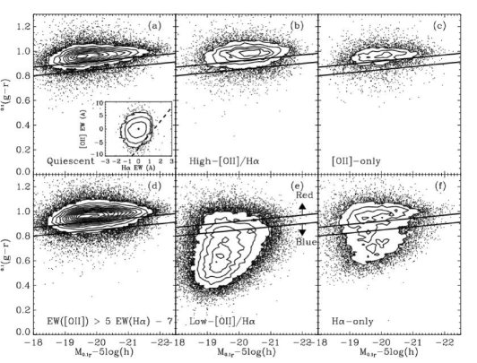
3. Galaxies with neither [O II] nor H$\alpha$ detected. We label these galaxies as “Quiescent Galaxies” in the remainder of this paper. Their EW measurements form a symmetric distribution around (0,0) in the [O II]-H$\alpha$ diagram and fall to the left of our demarcation, as shown in the inset plot of Fig. 4. As illustrated in Fig. 4, quiescent galaxies have a color-magnitude distribution very similar to the “High-[O II]/H$\alpha$” galaxies.

Fig. 4 shows the color-magnitude diagrams for these subsamples: quiescent galaxies (panel a), the high-[O II]/H$\alpha$ galaxies (b), [O II]-only galaxies (c), the low-[O II]/H$\alpha$ galaxies (e), and H$\alpha$-only galaxies (f). Our color cuts are drawn here as the two straight lines for references. Both the quiescent galaxies and the high-[O II]/H$\alpha$ galaxies display a highly symmetric red sequence. The quiescent galaxies have a wider luminosity range and the high-[O II]/H$\alpha$ galaxies have a slight asymmetry in color, but they are otherwise nearly indistinguishable in color-magnitude space. As shown in Fig. 5, they also have similar Sérsic index distributions. As expected, the [O II]-only galaxies have similar color-magnitude distributions and Sérsic index distributions as the high-[O II]/H$\alpha$ galaxies. The combination of the three subsamples shown in Fig. 4a-c – i.e., those galaxies to the left of the demarcation given by Eq. 6 on [O II]-H$\alpha$ diagram – together comprise a tight red sequence in the color-magnitude-concentration space, as shown in panel (d) of Fig. 4.

The low [O II]/H$\alpha$ subsample, as expected, covers the blue cloud in the color-magnitude diagram (Fig. 4d). However, it also includes some galaxies with red-sequence-like colors, especially at the faint end. These red galaxies within the low [O II]/H$\alpha$ sample, which in fact are the overflow points in the lower left panel of Fig. 2, also deserve special investigation. We will refer to them as “Red-Low-[O II]/H$\alpha$ galaxies”. As shown in Fig. 5, these galaxies generally have lower Sérsic indices than the overall red galaxy population. Their distribution does not resemble either of the possible parent samples; i.e., the red galaxy sample or the low-[O II]/H$\alpha$ sample. Thus, although these galaxies have red colors, they are likely to be a different population from the red sequence. The H$\alpha$-only galaxies (panel f) also extend to red colors. Without detection of [O II], their categorization is difficult; we will discuss them briefly later on. To recapitulate, we list in Table 1 our sample definitions and the fraction of each category in the volume-limited sample.

The [O II] EW distribution of all the galaxies to the left of the demarcation can be modeled well by the combination of a Gaussian distribution centered near zero and a log-normal distribution, as shown in Fig. 6. The two components correspond closely to the EW distributions of the quiescent population alone and the combined population of the high-[O II]/H$\alpha$ and the [O II]-only galaxies, respectively; the fractional area covered by the log-normal distribution (35.4%) is nearly identical to the fraction of galaxies with detectable [O II] emission (35.5%).

Figure 4.— Color-magnitude diagrams for the quiescent galaxies (a), the high-[O II]/H$\alpha$ galaxies (b), the [O II]-only galaxies (c), the galaxies to the left of the [O II]-H$\alpha$ demarcation (d), the low-[O II]/H$\alpha$ galaxies (e), and the H$\alpha$-only galaxies (f) in the magnitude limited sample ($0.05<z<0.10$). Quiescent galaxies, the high-[O II]/H$\alpha$ galaxies, and the [O II]-only galaxies all follow a tight red sequence. Low-[O II]/H$\alpha$ galaxies cover not only the blue cloud but also part of the red sequence region. Contours are plotted at number densities of $1.6\times 10^{4}n$ (halved in the panel b, c, and f) galaxies per mag², where $n$=1,2,…, starting from outermost contour. The inset in panel (a) shows the [O II]-H$\alpha$ EW distribution for the quiescent galaxies. They form a symmetric distribution around zero as expected.

Figure 5.— Sérsic index distributions of galaxies for four subsamples as defined in Table 1: high-[O II]/H$\alpha$ galaxies (thick-solid, height doubled for easy comparison), low-[O II]/H$\alpha$ galaxies (thick dashed), quiescent galaxies (thin-solid), and red-low-[O II]/H$\alpha$ galaxies (thin dashed). The high-[O II]/H$\alpha$ galaxies have a similar distribution to the quiescent galaxies, and very different from that of the low-[O II]/H$\alpha$ galaxies. The red-low-[O II]/H$\alpha$ galaxies have a distribution unlike either possible parent sample.

Figure 6.— The histogram shows the [O II] $\lambda$3727 EW distribution of all galaxies to the left of the demarcation (Eq. 6) in [O II]-H$\alpha$ diagram, including galaxies consistent with zero EW. It can be modeled well by the combination of a Gaussian distribution centered near zero (the dashed curve) and a log-normal distribution (the dot-dash curve). The sum of the two components is shown as the solid curve, which goes through the histogram. The EW distributions of all other emission lines in this subset of galaxies can be modeled the same way, with similar results. As in the rest of this paper,plotted EWs are the values after zero point correction (see Appendix B for details).

Name		Nonzero?		Criteria	Percentage
		[O II]	H$\alpha$
High-[O II]/H$\alpha$		Y	Y	${\rm EW}(\mbox{[{O~{}II}]})>5{\rm EW}(\mbox{H$\alpha$})-7$	13.3%
Low-[O II]/H$\alpha$		Y	Y	${\rm EW}(\mbox{[{O~{}II}]})<5{\rm EW}(\mbox{H$\alpha$})-7$	38.0%
	Red-Low-[O II]/H$\alpha$			(as low-[O II]/H$\alpha$, plus	(4.4%)
				${}^{0.1}(g-r)>-0.025(M_{{}^{0.1}r}-5\log h)+0.42)$
[O II]-only galaxies		Y	N		5.2%
H$\alpha$-only galaxies		N	Y		15.7%
Quiescent galaxies		N	N		27.9%

Table 1Subsample definitions and their fractions in the volume-limited sample; see §3.3 for details.

In the following section, we employ more line ratio diagnostics to investigate the source of the emission lines in red galaxies, specifically, the High-[O II]/H$\alpha$ population and the Red-Low-[O II]/H$\alpha$ population.

4. Origin of [OII] emission in red galaxies

4.1. Classifications by line ratio diagnostics

Emission lines in galaxy spectra can be produced by a variety of mechanisms; Among them, photoionization by AGN and by hot stars in star-forming HII regions are two major mechanisms. Baldwin, Phillips and Terlevich (1981, hereafter BPT) pioneered the use of intensity ratios of two pairs of emission lines to distinguish starforming galaxies from AGNs. The method was further developed by Veilleux & Osterbrock (1987). The so-called BPT diagram of line ratios, such as the one shown in the panel (a) of Fig. 7, has become a standard tool for determining the source of line emission.

All the galaxies plotted in Fig. 7 have at least 2$\sigma$ detections of all emission lines considered (H$\beta$, [O III] $\lambda$5007, H$\alpha$, [N II] $\lambda$6583). Two sequences of emission-line galaxies dominate this diagram; one corresponds to the star-forming galaxies, and the other to AGN. The star-forming sequence is the curved concentration of points that extends from center bottom to upper left; its shape reflects the correlation between ionization parameter and metallicity in star-forming galaxies (Kewley et al. 2001). The concentration of points on the right part of the plot is identified with AGNs (e.g., Baldwin et al. 1981; Veilleux & Osterbrock 1987; Kauffmann et al. 2003). In studies employing optical emission lines from large aperture spectroscopy, one usually cannot confirm that the emission lines are associated with a central supermassive black hole. From now on, we define a “true AGN” as a system in which the radiation is ultimately powered by accretion onto a supermassive black hole. In the remainder of this paper, we will refer to galaxies with line ratios characteristic of true AGN as “AGN-like galaxies”.

The theoretical modeling of starburst galaxies can produce a boundary for the locus of star-forming galaxies on the BPT diagram, which is called the extreme starburst classification line. The classification line given by  Kewley et al. (2001) is indicated by the solid curve in Fig. 7. As seen in this figure, that would serve as a very conservative cut for selecting AGN-like galaxies. An alternative empirical demarcation has been suggested by Kauffmann et al. (2003), which is indicated by the dashed curve in Fig. 7.

Traditionally, AGNs are further divided into several sub-categories according to their positions in the BPT diagram: Seyferts, Low-Ionization Nuclear Emission-line Regions (LINERs) and Transition Objects (TOs). Traditional definitions for Seyferts and LINERs are indicated by the horizontal and vertical lines (Shuder & Osterbrock 1981; Veilleux & Osterbrock 1987) in Fig. 7. Ever since the discovery of LINERs (Heckman 1980), it has remained uncertain whether they are true AGN. Recently, it has become clear that at least some LINERs are indeed accretion-powered systems (Filippenko 2003; Ho 2004, and references therein). However, LINER-type line ratios are also found coming from extended regions in some early-type galaxies (Heckman et al. 1989; Goudfrooij et al. 1994; Goudfrooij 1999), in support of other ionization mechanisms, such as shockwaves, cooling flows, hot old stars, etc. Transition Objects are galaxies that satisfy most of the LINER criteria but have weaker [O I] $\lambda$6300/H$\alpha$ ratio (Filippenko & Terlevich 1992; Ho et al. 1993). The dividing line between LINERs and TOs in [O I]/H$\alpha$ is indicated by the vertical dashed line in Fig. 8, which shows another useful BPT diagram with [O III] $\lambda$5007/H$\beta$ plotted against [O I] $\lambda$6300/H$\alpha$. The nature of Transition Objects still remains unclear.

Figure 7.— (a) Line ratio diagnostic diagram (BPT diagram) showing the emission-line flux ratio [O III]/H$\beta$ versus the ratio [N II]/H$\alpha$ for the magnitude-limited sample ($0.05<z<0.1$). This BPT digram, by construction, is very insensitive to the effects of extinction. All galaxies plotted have at least 2$\sigma$ detection on all four emission lines used. The solid curve shows the demarcation defined by Kewley et al. (2001) to separate star-forming galaxies from AGN. The dashed curve shows the demarcation used by Kauffmann et al. (2003). Conventional dividing lines for Seyferts and LINERs are indicated by the horizontal and vertical lines (Shuder & Osterbrock 1981; Veilleux & Osterbrock 1987). Contours are plotted at number densities of $24,000n$ galaxies per unit area, where $n$=1,2,…, starting from the outermost contour. (b) Same diagram as panel (a) but only High-[O II]/H$\alpha$ galaxies are shown. These are centered in the LINER region. The $1\sigma$ measurement errors propagated to log-line-ratio is shown as the cross. Contours are plotted at number densities of $8,000n$ galaxies per unit area, where $n$=1,2,… . (c) Same diagram for the Red-Low-[O II]/H$\alpha$ sample. They lie to the left of the LINER region and extend down to the star-forming region. Other than the Seyferts and the star-forming galaxies, most are Transition Objects, as shown in Fig. 8. Contours indicate the same number density levels as in panel (b).

Figure 8.— (a) BPT diagram showing the emission-line flux ratio [O III] $\lambda$5007/H$\beta$ versus the ratio [O I] $\lambda$6300/H$\alpha$ for the magnitude-limited sample ($0.05<z<0.1$). The effect of $A_{V}=2$ of extinction (for $R_{V}=3.1$) is indicated by the little arrow. All galaxies plotted here have at least 2$\sigma$ detections on all four emission lines. The solid curve shows the demarcation defined by Kewley et al. (2001) to separate star-forming galaxies (to the left and below) from AGN (to the right and above). The horizontal line is the dividing line between Seyferts (above) and LINER/TOs (below) as defined by Shuder & Osterbrock (1981) and Veilleux & Osterbrock (1987). Contours indicate number density levels of $10,000n$ ($n$=1,2,…) galaxies per unit area. (b) The same diagram for the High-[O II]/H$\alpha$ sample. The vertical line is the dividing line between Transition Objects and LINERs given by Ho et al. (1997a). The High-[O II]/H$\alpha$ sample lies almost entirely in the LINER region, with scatter similar to the measurement errors. The $1\sigma$ measurement errors propagated to log-line-ratio is shown as the cross. Contours indicate number density levels of $2,400n~{}(n=1,2,...)$ galaxies per unit area. (c) The same diagram for the Red-Low-[O II]/H$\alpha$ sample. These objects lie to the left of the TO/LINER dividing line and thus are indeed Transition Objects, plus a few Seyferts and star-forming galaxies. Contours indicate the same number density levels as in panel (b).

Now we examine the position of the two classes of red galaxies in the BPT diagrams. We look at the High-[O II]/H$\alpha$ sample and the Red-Low-[O II]/H$\alpha$ sample separately because they have different [O II]-H$\alpha$ correlations. In the two BPT diagrams (Fig. 7 & 8), the two samples are displayed by themselves in panels (b) and (c). In both BPT diagrams, the High-[O II]/H$\alpha$ sample (panel b) has a nearly symmetric distribution centered on the region classified as LINERs. The scatter is due to intrinsic variations as well as measurement errors. The median errors are indicated on the plot. Galaxies in the Red-Low-[O II]/H$\alpha$ sample mostly fall into the transition region in both BPT diagrams (panel (c) in each). Fig. 8 shows clearly that most of these galaxies are in fact Transition Objects as defined by Ho et al. (1997a), while a smaller fraction are Seyferts and star-forming galaxies.

Comparing [O II] $\lambda$3727 with [O I] $\lambda$6300, one can see the similarity in their relations to H$\alpha$: both [O II]/H$\alpha$ and [O I]/H$\alpha$ ratios provide a separation between LINERs and other categories. In fact, the bimodality in [O I]/H$\alpha$ is employed in one of the BPT diagrams to distinguish AGNs from star-forming HII regions. Unfortunately, [O I] $\lambda$6300 is often too weak to detect, which hinders the use of this particular BPT diagram for the full sample. As we have shown above, the strong bimodality in EW([O II])/EW(H$\alpha$) (or similarly, EW([O II])/EW(H$\beta$) ) might make it a good alternative, despite the wide separation of the two lines in wavelength. We propose the use of the demarcation in the EW([O II])-EW(H$\alpha$) plane shown in Fig. 2 to separate LINER-like galaxies from other line-emitting objects.

Not all of the high-[O II]/H$\alpha$ galaxies are plotted on the two BPT diagrams(Fig. 7 & 8). Because [O I] $\lambda$6300 and H$\beta$ are much weaker than strong emission lines like [O II] $\lambda$3727 and H$\alpha$, requiring them to be detected significantly reduces the sample size, especially among the high-[O II]/H$\alpha$ population. Do such requirements bias our sample selection? We test this with a BPT diagram (Fig. 9) which only involves the strong lines: [O III]/[O II] vs. [N II]/H$\alpha$. Panel (a) of Fig. 9 shows the distribution for all galaxies with at least 2-$\sigma$ detections on all of the four strong lines. Galaxies identified as star-forming from other BPT diagrams are again found from bottom to middle left. The horizontal line indicates the [O III]/[O II] division originally defined by Heckman (1980) to separate LINERs from Seyferts. The vertical line is a commonly adopted limit for separating LINERs and Seyferts from star-forming galaxies (e.g., Ho et al. 1997a). In panel (b) of Fig. 9, only high-[O II]/H$\alpha$ galaxies are plotted. It is worth noting that the high-[O II]/H$\alpha$ galaxies again fall into the LINER region. In panel (c), we only plot high-[O II]/H$\alpha$ galaxies which also have at least 2-$\sigma$ detections on [O I] and H$\beta$, i.e., those which are also plotted in Fig. 7 & 8. These galaxies have very similar distributions as those without detectable [O I] or H$\beta$, only biased slightly against high [N II]/H$\alpha$ ratio and high [O III]/[O II] ratio. The former is likely due to the difficulty of measuring H$\beta$ for galaxies with very low H$\alpha$ and thus high [N II]/H$\alpha$ ratio. The latter is probably due to the difficulty of measuring [O I] for galaxies with relatively high ionization. Thus, requiring [O I] and H$\beta$ detections only biases the sample slightly, and in expected ways. We thus believe that nearly all high-[O II]/H$\alpha$ galaxies have LINER-like line ratios, regardless of their [O I] or H$\beta$ detectability.

Figure 9.— (a) Line ratio diagnostic diagram (BPT diagram) showing the emission-line flux ratio [O III]/[O II] versus the ratio [N II]/H$\alpha$ for the magnitude-limited sample ($0.05<z<0.1$). All galaxies plotted have at least 2$\sigma$ detections on all four emission lines. Traditional definitions for Seyferts and LINERs are indicated by the horizontal and vertical lines (Heckman 1980; Shuder & Osterbrock 1981; Veilleux & Osterbrock 1987). Contours are plotted at number densities of $45,000n$ galaxies per unit area, where $n$=1,2,…. . The effect of $A_{V}=2$ of extinction (for $R_{V}=3.1$) is indicated by the arrow. (b) Same diagram as panel (a) but only High-[O II]/H$\alpha$ galaxies are shown. These are centered in the LINER region. The $1\sigma$ measurement errors propagated to log-line-ratio is shown as the cross. Contours are plotted at number densities of $25,000n$ galaxies per unit area, where $n$=1,2,… . (c) Same diagram but only high-[O II]/H$\alpha$ galaxies which also have at least 2$\sigma$ detections on [O I] and H$\beta$ are plotted. They have similar distributions as those without detectable [O I] or H$\beta$, only biased slightly against high [N II]/H$\alpha$ ratio and high [O III]/[O II] ratio.

The high-[O II]/H$\alpha$ galaxies, as shown above, have relatively uniform line ratios in [O II]/H$\alpha$, [O III]/H$\beta$, [N II]/H$\alpha$, [O I]/H$\alpha$, and [O III]/[O II], which altogether identify them as LINER-like. As found in §3.3, the high-[O II]/H$\alpha$ galaxies occupy the same region in the color-magnitude space as quiescent galaxies do and they share the same distribution in galactic concentration. Since they only differ in emission line strengths, we speculate that these LINER-like galaxies have a close evolutionary relationship with the quiescent red sequence galaxies. They might be the immediate progenitors of the quiescent red galaxies — a scenario in which the LINER phase lasts for some period of time when the galaxy first arrives on the red sequence (Graves et al., in prep). Alternatively, it could be that LINER phases are intermittent throughout the life of a quiescent galaxy. As pointed out in §3.3, the combination of the LINER-like (high-[O II]/H$\alpha$) galaxies and the quiescent galaxies produces a uniform red sequence; the red sequence is effectively a LINER/Quiescent sequence.

We turn now to the low-[O II]/H$\alpha$ galaxies. As was the case previously, not all of the low-[O II]/H$\alpha$ galaxies are plotted on the BPT diagrams because of S/N limitations. But as we found before, in the [O III]/[O II] vs. [N II]/H$\alpha$ diagram, the distribution of red-low-[O II]/H$\alpha$ galaxies is also found to be independent of their [O I] or H$\beta$ detectability. Their line ratios vary from star-forming, to Transition Objects, to Seyferts. To quantify the relative fraction of each category, we use [N II]/H$\alpha$ ratio, which is most commonly detectable among this population. As listed in Table 2, a little more than 1/3 of these have $\mbox{[{N~{}II}]}/\mbox{H$\alpha$}<0.6$, similar to dusty star-forming galaxies, while the rest have $\mbox{[{N~{}II}]}/\mbox{H$\alpha$}>0.6$, resembling TO/Seyferts.

The [O II]-only galaxies likely belong to the high-[O II]/H$\alpha$ category intrinsically, as they occupy the same color-magnitude space, have the same Sérsic index distribution, and have lower limits on [O II]/H$\alpha$ ratio higher than typical high-[O II]/H$\alpha$ galaxies. Therefore, we suspect they also belong to the LINER-like category.

The case for the H$\alpha$-only galaxies is more complicated, since the ratio of the EWs at which [O II] and H$\alpha$ are detectable is similar to the [O II]/H$\alpha$ EW ratio of a typical high-[O II]/H$\alpha$ galaxy. The H$\alpha$-only population will include both high-[O II]/H$\alpha$ and low-[O II]/H$\alpha$ galaxies. Among them, we can only separate star-forming galaxies out using the [N II]/H$\alpha$ ratio, the only line ratio available in most of these galaxies; see Table 2.

Previous studies of emission lines in early-type galaxies had already shown that [O II] $\lambda$3727 emission is detected in roughly half of all early-type galaxies (Mayall 1958; Caldwell 1984; Phillips et al. 1986). Most of these galaxies in which multiple emission lines are detected have LINER-like line ratios (Phillips et al. 1986; Goudfrooij et al. 1994; Zeilinger et al. 1996). With a much bigger sample, we find from SDSS data that $\sim 38\%$ of all red galaxies in the volume-limited sample have [O II] $\lambda$3727 positively detected. As shown above, the red-sequence population actually has two major sub-components: the LINER/Quiescent sequence and the TO/Seyferts. The former dominates the red galaxy population; the LINER-like population is one of the two main components in the [O II]-H$\alpha$ bimodality. Table 2 gives the detailed population breakdown of red galaxies in the volume-limited sample. Emission lines are detected in 52.2% of all red galaxies; LINER-like galaxies comprise at least 28.8%, dusty-starforming galaxies comprise about 6.5%, while TOs and Seyferts are less than 16.8%.

Nonzero?		[O II]/H$\alpha$	Number	Percentage	Category
[O II]	H$\alpha$
N	N		12913	47.8%	Quiescent
N	Y	Uncertain	3886	14.4%	LINERs, TOs and Seyferts ([N II]/H$\alpha$ $>0.6$, 11.1%); Dusty SF ([N II]/H$\alpha$ $<0.6$, 3.2%)
Y	N	High	2209	8.2%	Possibly LINER-like
Y	Y	High	5571	20.6%	LINER-like
		Low	2421	9.0%	TOs and Seyferts ([N II]/H$\alpha$ $>0.6$, 5.7%); Dusty SF ([N II]/H$\alpha$ $<0.6$, 3.3%)
Total			27000	100%	All red galaxies

Table 2Detailed population breakdown of red galaxies in the volume limited sample, see §4.1.

4.2. Possible Sources of the Emission in High-[O II]/H$\alpha$ Galaxies

As discussed in the introduction, many recent studies suggest that star formation could contribute substantially to the [O II] and H$\beta$ emission in Type II QSOs and Seyfert 2 galaxies. Is this also the case for LINERs? We have shown in §3.2 that the [O II]-H$\alpha$ ratio in the high-[O II]/H$\alpha$ population cannot be reached by star formation alone. Here, we provide additional evidence using a BPT-like diagram involving [O II] $\lambda$3727 to show that star formation does not contribute substantially to [O II] emission in these galaxies.

First we redivide our emission-line galaxies into four categories: star-forming galaxies, Seyferts, LINERs, and Transition Objects, using definitions similar to the conventions used in the literature. Our classification scheme is illustrated in Fig. 10. We first employ the demarcation proposed by Kauffmann et al. (2003) to separate star-forming galaxies from other categories. Then we define Seyferts conventionally as galaxies with [O III] $\lambda$5007/H$\beta$ $>3$. The remaining region belongs to LINERs and TOs. We adopt the definition in Ho et al. (1997a) to define LINERs as objects with $\mbox{[{O~{}I}] $\lambda$6300}/\mbox{H$\alpha$}>0.17$ and TOs as objects with $\mbox{[{O~{}I}] $\lambda$6300}/\mbox{H$\alpha$}<0.17$.

Figure 10.— This diagram shows the definition scheme described in §4.2 and used in Fig. 11. We first employ the demarcation proposed by Kauffmann et al. (2003) to separate star-forming galaxies from other categories. Then we define Seyferts conventionally as galaxies with [O III] $\lambda$5007/H$\beta$ $>3$ (Shuder & Osterbrock 1981; Veilleux & Osterbrock 1987). Last, we adopt the definition in Ho et al. (1997a) to separate LINERs and TOs using their [O I] $\lambda$6300/H$\alpha$ ratio.

Fig. 11 shows a BPT-like diagram with the [O II] $\lambda$3727/H$\beta$ ratio plotted against the [N II] $\lambda$6583/H$\alpha$ ratio. A comparison between panel (a) and panel (c) shows clearly that LINER-like galaxies have no overlap with star-forming galaxies. If, for instance, star formation contributes substantially to the [O II] emission in LINERs, it will also contribute to H$\beta$ in proportion according to a star-forming ratio. As a result, the [O II]/H$\beta$ ratio and [N II]/H$\alpha$ ratio would be displaced towards the region occupied by star-forming galaxies. In fact, the LINERs have very little vertical overlap with star-forming galaxies in [O II]/H$\beta$ ratio. Interestingly, Seyferts and Transition Objects do have huge overlap with star-forming galaxies, which is consistent with the picture that some of them might have substantial fractions of their [O II] and H$\beta$ emission contributed by HII regions. Note LINER-like galaxies all fall in the high-[O II]/H$\beta$ category, which is roughly equivalent to the high-[O II]/H$\alpha$ category. In fact, LINER-like galaxies have the highest [O II]/H$\beta$ ratios observed. Thus it is impossible to produce LINER-like line ratios by combining Seyferts and HII region spectra.

It is logically possible that pure LINERs have more extreme ratios and star formation contribution brought them down to the current positions in the line ratio diagram. If that were true, the star formation rate would have to be remarkably uniform among all LINERs. Otherwise, we would see a spread of emission line ratios, producing an elongated distribution like those for Seyferts and Transition Objects. Thus this scenario is highly unlikely.

Figure 11.— BPT-like diagrams showing [O II] $\lambda$3727/H$\beta$ plotted against [N II] $\lambda$6583/H$\alpha$. The positions of star-forming galaxies (panel a), Seyferts (b) and LINERs (c) are shown separately. The effect of $A_{V}=2$ of extinction (for $R_{V}=3.1$) is indicated by the arrow in panel a. There is very little vertical overlap between LINERs and star-forming galaxies in [O II]/H$\beta$ ratio, which shows that star formation do not contribute substantialy to the [O II] and H$\beta$ emission in LINERs. Note LINERs all fall in the high-[O II]/H$\beta$ (equivalent to high-[O II]/H$\alpha$) category.

It is therefor clear that the high-[O II]/H$\alpha$ mode in the bimodality is mainly composed of LINERs and the line emission is produced by mechanisms other than star formation. However, the exact ionization mechanism for emissions with LINER-type line ratios is uncertain. The definition of LINER, as indicated by its name, refers only to emission regions around the nucleus of a galaxy, but LINER-like line ratios have also been observed in extended emission-line regions (Phillips et al. 1986; Heckman et al. 1989; Goudfrooij et al. 1994; Zeilinger et al. 1996; Goudfrooij 1999; Sarzi et al. 2005, Graves et al. in prep). Since SDSS spectra were taken with 3” fibers, which cover a region $\sim 4{\rm kpc/h}$ in diameter at the median redshift of our sample, both the nuclei and possible extended emission regions in the galaxies would be included. Thus, we cannot tell whether the line emission in these red galaxies is associated with compact nuclear sources, extended regions, or both.

However, the occurence of LINER-like line ratios in SDSS data is roughly consistent with results from the Palomar survey (Filippenko & Sargent 1985; Ho et al. 1997a, b), which was conducted with a similar aperture (2”x4”) but targeted very nearby galaxies, therefore probing much smaller regions $\sim 100$ parsec in diameter. Using that dataset, Ho et al. (1997b) found that $\sim 30\%$ of early-type galaxies host a LINER. In the present SDSS sample, a similar fraction, namely $>29\%$, of red galaxies have LINER-like emission line ratios. We thus expect that if emission from extended regions dominates the lines we observe, its line ratios and strengths must still correlate well with emission from the galaxies’ nuclei.

Besides photoionization by a central non-stellar source, such as an accretion-powered system (Ferland & Netzer 1983; Halpern & Steiner 1983; Groves et al. 2004b), many ionization mechanisms have been proposed to explain the LINER- and TO-like optical emission in early-type galaxies: (1) photoionization by the X-rays radiated as hot gas cools (Voit & Donahue 1990; Donahue & Voit 1991; Kim 1989), (2) heat transfer from hot gas to cooler gas (Sparks et al. 1989), (3) collisional excitation by shock waves (Heckman et al. 1989; Dopita & Sutherland 1995), (4) photoionization from some component of the stellar population, such as post-AGB stars (di Serego Alighieri et al. 1990; Binette et al. 1994). We have compared the line ratios in the LINER-like SDSS galaxies with theoretical predictions of both shockwave models (Dopita & Sutherland 1995, 1996) and the lowest-ionization Seyfert photoionization models (Groves et al. 2004a, b). Both models produce line ratios roughly consistent with the observed ones. Detailed comparisons also require a careful extinction correction (given the possibility of patchiness) and metallicity measurements, which are beyond the limits of this paper. To reliably distinguish these different mechanisms, more information than just line ratio is needed, such as the spatial extent and kinematics of the emission-line regions, the spatial variation of line ratios, correlation with X-ray, UV and radio properties, etc. It is also quite possible that many of these mechanisms are involved. This is beyond the scope of the current paper, and as such we do not try to answer this question here.

5. Implications for Studies of Post-starburst Galaxies

H$\alpha$ luminosity, the best optical indicator of star formation rate, is very difficult to measure at $z>0.5$ due to atmospheric emission in the near infrared. Instead [O II] $\lambda$3727 luminosity is commonly used (Dressler & Gunn 1983; Zabludoff et al. 1996; Hammer et al. 1997; Hogg et al. 1998; Dressler et al. 1999; Poggianti et al. 1999; Balogh et al. 1999; Rosa-González et al. 2002; Tran et al. 2003; Hippelein et al. 2003; Yang et al. 2004; Tran et al. 2004). However, we have shown above that the origin of [O II] in most red galaxies is not star formation. This could have strong consequences for the definition of post-starburst galaxy samples, as they are approaching the red sequence and could suffer the same issues.

Figure 12.— Top panel: The distribution of H$\alpha$ EW vs. A/K ratio for all galaxies with $0.05<z<0.2$ in the SDSS DR4 main galaxy sample that have both [O II] and H$\alpha$ covered in their spectra (compare to Fig.3 in Quintero et al.). Post-starburst galaxies comprise a distinct population and stand out as the horizontal spur with nearly zero H$\alpha$ EW but relatively large A/K ratio. The empirical selection criteria are shown with the two solid lines. Bottom panel: The distribution of [O II] EW vs. A/K ratio for the same sample. The horizontal spur apparent in the top panel disappears. The dark points indicate the positions in the bottom panel of post-starburst galaxies selected in the top panel. These galaxies span a wide range in [O II] EW and overlap with the region occupied by star-forming galaxies.

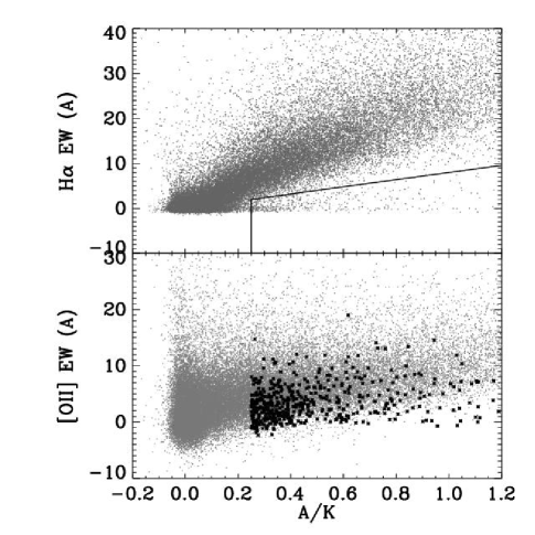
Quintero et al. (2004) have demonstrated that post-starburst galaxies in the SDSS sample comprise a distinct population in a plot of H$\alpha$ EW against A/K ratio. The H$\alpha$ EW provides a measure of the current specific SFR in a galaxy, while the A/K ratio is linked to the average specific SFR over the past 1 Gyr; comparing these two quantities indicates how the SFR is changing. In the top panel of Fig. 12, we reproduce Fig.3 of Quintero et al. with our own measurements for all galaxies that are within $0.07<z<0.1$ and have both [O II] and H$\alpha$ visible in their spectra. For most galaxies, the two star formation indicators are highly correlated, as one would expect. Post-starburst galaxies stand out as the horizontal spur with nearly zero H$\alpha$ EW but relatively large A/K, i.e., they have little or no current SFR but large recent SFR. Alert readers will notice the difference between our A/K measurement from that of Quintero et al.’s; our linear decomposition is done after the subtraction of a continuum, while theirs is done without continuum subtraction; the templates used also differ. In spite of this, the post-starburst population remains identifiable. We define post-starbursts as galaxies satisfying three criteria: ${\rm A/K}>0.25$, $\mbox{H$\alpha$}\ {\rm EW}<8({\rm A/K})$ and $\mbox{H$\alpha$}\ {\rm EW}<10{\rm\AA}$.

If we replace H$\alpha$ by [O II], as shown in the bottom panel of Fig. 12, the post-starburst spur disappears. Although they have minimal H$\alpha$ emission, post-starburst galaxies span a wide range of [O II] EW. In a plot of [O II] EW vs. A/K ratio, post-starburst galaxies identified using H$\alpha$ overlap with the region occupied by star-forming galaxies, as seen in the lower panel of Fig. 12.

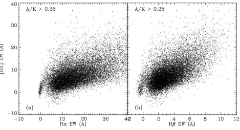
The left panel of Fig. 13 shows more directly what causes the difference between the two panels of Fig. 12. This figure replots Fig. 2 but using only galaxies with an A/K greater than 0.25. This corresponds to the A/K cut Quintero et al. (2004) used to define their post-starburst (K+A) sample; in this plot, we include all galaxies regardless of H$\alpha$ EW. As expected, most galaxies on the star-forming sequence from Fig. 2 remain, while most red galaxies are excluded. However, there is a small group of points forming a vertical spike near zero H$\alpha$ EW; these are post-starburst galaxies having high A/K and little or no H$\alpha$ emission. There is a gap in H$\alpha$ that naturally separates this post-starburst population from star-forming galaxies. However, there exists no corresponding gap in [O II] EW.

In fact, roughly 50% of post-starburst (K+A) galaxies identified using H$\alpha$ belong to either the high-[O II]/H$\alpha$ population or the [O II]-only population defined in §3; the remainder are classified as quiescent. Although they show minimal H$\alpha$ emission, they have LINER/AGN-like line ratios, and can have appreciable [O II] emission. Thus, H$\alpha$ can be used as a universal star formation indicator for most cases with little contamination. However, in red and post-starburst galaxies, LINER/AGN can possess [O II] lines as strong as those in star-forming galaxies.

Figure 13.— Left: [O II] EW vs. H$\alpha$ EW distribution for galaxies with $A/K>0.25$; i.e., those with relatively young stellar populations. Compare to Fig. 2a. However, here we include all EW measurements regardless of the signal-to-noise of the detection. Right: same galaxies as in left panel, but with H$\beta$ EW on the x-axis. In the H$\beta$ distriubtion, although EWs are smaller and measurement errors are larger than for H$\alpha$, the separation between post-starburst and star-forming galaxies remain apparent.

For this reason, using [O II] to identify post-starbursts is problematic. Adopting a low [O II] EW cut would make the selection heavily incomplete, while a high cut would bring huge contamination from star-forming galaxies. In addition, differing levels of measurement errors will cause varying degrees of contamination. This could well explain the drastically different post-starburst abundances found in some previous studies (Dressler et al. 1999; Poggianti et al. 1999; Balogh et al. 1999). In the volume-limited sample, 66% of post-starburst galaxies have detectable [O II] emission; 57% have [O II] EW greater than 2.5Å. Previous studies which used an [O II] EW cut of this level could be missing half of all the post-starbursts.

Unlike [O II], H$\alpha$ appears to provide a generally reliable indication of the presence of star formation in the absence of a full BPT diagnosis. However, at $z>0.4$, H$\alpha$ is difficult to measure due to strong atmospheric emission and declining instrumental sensitivity. [O II] has been used as a proxy for measuring SFR at redshifts up to $z\sim 1.4$, but as shown above, it is problematic for red and post-starburst galaxies. In its place, we suggest the use of H$\beta$, which is available out to higher redshifts than H$\alpha$, but is much more reliable for red galaxies than [O II]. In the DEEP2 Galaxy Redshift Survey (Davis et al. 2003), H$\beta$ can be measured up to $z\sim 0.9$, enabling a direct comparison with low-z studies. Although it is much weaker than H$\alpha$, more affected by dust, and has a deeper stellar absorption component to remove, H$\beta$ behaves similarly to H$\alpha$ in SDSS data, as shown in the right panel of Fig. 13. In a future paper, we will use H$\beta$ to identify post-starburst galaxies in DEEP2 and compare with low-z results. Finally, for completeness, we also give an empirical bimodality demarcation for [O II]-H$\beta$:

$${\rm EW}(\mbox{[{O~{}II}]})=18{\rm EW}(\mbox{H$\beta$})-6.$$ (7)

5.1. The Nature of Post-starburst emission

Tradiationally, post-starburst galaxies have been defined as galaxies with no detectable line emission. Quintero et al. (2004) enlarged the definition to include galaxies with nonzero H$\alpha$ emission but too weak compared to star-forming galaxies with a similar fraction of young stars (similar A/K ratio, see Fig. 12). As shown above, these galaxies can have rather strong [O II] lines, even when H$\alpha$ is not detectable (consistent with zero). In the volume-limited sample, 78% of post-starburst galaxies have at least one emission line detected at $>2\sigma$ significance. What is the nature of this emission? Does it indicate residual star formation?

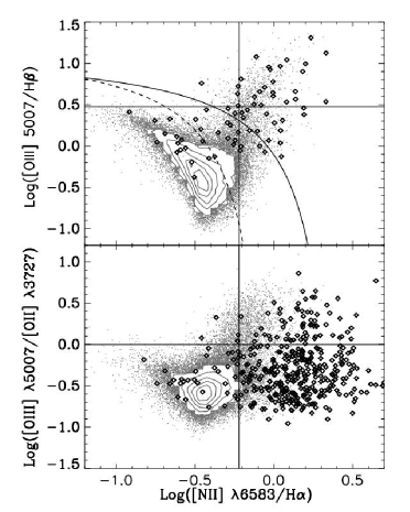
For post-starbursts that have reliable line detections, we can again employ BPT diagrams to study the nature of their emission. Fig. 14 shows two BPT diagrams for galaxies with A/K greater than 0.25 in the magnitude-limited sample ($0.05<z<0.1$), i.e., only galaxies which contain young stellar populations. As before, we require a minimum detection of 2$\sigma$ on all lines, which excludes some fraction of the post-starburst galaxies from the diagrams depending on the lines used. For example, about 1/3 of all post-starbursts are included in the bottom panel but only 5% in the top panel. As shown in this figure, most post-starburst galaxies in which all emission lines involved are positively detected show AGN-type line ratios and cover all categories of AGN – LINER, TO, and Seyfert. Only 6% of these post-starbursts show line ratios characteristic of star-forming HII regions, which also turn out to be preferentially high-H$\alpha$ EW cases.

Those post-starbursts that cannot be plotted on the BPT diagram mostly belong to the high-[O II]/H$\alpha$ group, the [O II]-only group, or the quiescent group. Of the $\sim 20\%$ low-[O II]/H$\alpha$ and H$\alpha$-only galaxies, the majority have [N II]/H$\alpha$$>0.6$ suggesting a non-starforming origin for the emission lines.

We can break down the classifications for all post-starbursts following the scheme used in Table 2 and use the [O II]-H$\alpha$ demarcation and [N II]/H$\alpha$ ratio to discriminate between star-forming galaxies and other groups. We find only 5% of post-starbursts in the volume limited sample have emission lines dominated by residual star formation. Instead, the emission in most post-starbursts has AGN-like line ratios. Recently, much evidence has suggested a connection between AGN and post-starbursts (Brotherton et al. 1999; Canalizo & Stockton 2001; Kauffmann et al. 2003; Heckman 2004; Ho 2005). Do AGN play a role in quenching star formation? The fact that post-starbursts have AGN-like line ratios is consistent with this picture.

Conservatively speaking, without knowledge of the spatial distribution of emission and information from other wavebands, we cannot conclude definitely that these are true AGNs. Unlike most red, elliptical galaxies, post-starburst galaxies have young stellar populations, which allow at least one more candidate excitation mechanism for LINER-type line ratios aside from those described above in §4.2. Taniguchi et al. (2000) point out that hot planetary nebula nuclei formed 100-500Myr following a starburst could provide the ionizing spectra necessary to form LINER-type emission lines. Further observations of post-starburst galaxies in other wavebands and more detailed modeling should provide a final answer to this question. If AGNs are in fact ubiquitous among post-starburst galaxies, it may provide a hint that AGN played a role in the quenching of their star formation.

Figure 14.— Line ratio diagnostic diagrams for galaxies with $A/K>0.25$ in the magnitude limited sample: [O III] $\lambda$5007/H$\beta$ vs. [N II] $\lambda$6583/H$\alpha$ (top) and [O III] $\lambda$5007/[O II] $\lambda$3727 vs. [N II] $\lambda$6583/H$\alpha$ (bottom). All galaxies plotted here have at least 2$\sigma$ detections on the emission lines involved. Post-starburst galaxies are highlighted with the diamond symbol; they mostly have LINER-type line ratios. The number of post-starburst galaxies plotted in the top panel is much smaller because H$\beta$ is more difficult to detect than the strong lines used in the bottom panel.

6. Summary

We have measured the fluxes and EWs of [O II], H$\alpha$  and several other emission lines for $\sim 300,000$ galaxies in the SDSS DR4 main galaxy sample after careful subtraction of the stellar continua. From the comparison between [O II] and H$\alpha$, combined with a variety of line ratio diagnostics, we have investigated the origin of line emission in red galaxies and the implications for post-starburst galaxy studies. Our main conclusions are as follows:

1. Galaxies display a bimodality in [O II]/H$\alpha$ ratio, which corresponds closely to the bimodality in their rest-frame colors. In blue galaxies, the [O II]/H$\alpha$ ratio generally matches the expectation for star-forming HII regions. However, in most red galaxies, the [O II]/H$\alpha$ ratio is unusually high and difficult to reconcile with predictions for star-forming HII regions.

2. About 52% of all red galaxies have detectable line emission; 38% have detectable [O II] $\lambda$3727 emission. More than 29% of all red galaxies have line ratios characteristic of LINERs, while less than 17% are TOs or Seyferts, and $\sim 6\%$ have lines dominated by star formation (probably dusty starbursts and edge-on spirals). Further information about the spatial distribution of emission in these galaxies and/or X-ray, UV and radio observation is necessary to firmly identify the origin of the line emission in each case.

3. LINER-like galaxies make up the high-[O II]/H$\alpha$ mode in the [O II]/H$\alpha$ bimodality. Other than modest differences in the luminosity range spanned, they are essentially indistinguishable from quiescent galaxies in the color-magnitude-concentration space. The combination of LINER-like and quiescent galaxies defines a uniform red sequence in color-magnitude-concentration space, which can be effectively selected by a simple division in the [O II]-H$\alpha$ EW diagram. The remaining red galaxies, those with low [O II]/H$\alpha$ ratio, are mostly TOs, dusty-starforming galaxies, and a small fraction of Seyferts. This group also have lower galactic concentration and slightly bluer color than the LINER/Quiescent red sequence.

4. Post-starburst galaxies, identified in the SDSS dataset using a lack of H$\alpha$ emission to indicate that star formation has ceased, often exhibit significant [O II] EW. Their positions in the [O II]-H$\alpha$ plot and BPT diagrams are the same as for Seyferts, LINERs and TOs, which suggest they may harbor AGNs. Less than 5% of this post-starburst sample show evidence for residual star formation.

5. [O II] emission in red galaxies and in post-starburst galaxies (i.e., in cases where it is not induced by star-formation) can be as strong as in star-forming galaxies. Locally at least, [O II] can only be used as a star-formation indicator for blue galaxies.

6. More than half of all the post-starbursts have detectable [O II] emission. Post-starburst samples defined using [O II] as a star-formation indicator will be very incomplete, especially if AGN/LINER rates and intensity were higher in the past. We recommend using H$\beta$ as an alternative for high-redshift studies.

Appendix A Stellar continuum subtraction

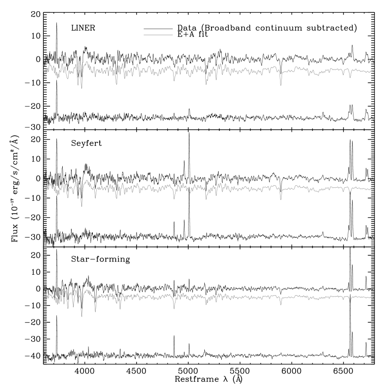
To get an accurate measurement of the emission line fluxes and equivalent widths, we need to subtract the stellar component underneath. All Balmer lines have a broad absorption component, while the continuum underlying [O II] has many narrower absorption features. The best way of removing the stellar component is often to fit the entire spectrum with a stellar population synthesis model. Here, we trade off this freedom for robustness and efficiency.

Instead of doing full population synthesis modeling, we decompose the spectra into two components: an old stellar population and a young stellar population. Similar methods have been used in modeling the spectra of E+A galaxies, such as in Quintero et al. (2004), who employed an A-star spectrum and a composite luminous red galaxy spectrum as templates. As pointed out by Dressler & Gunn (1983), a linear combination of the two components can simultaneously reproduce both the broad spectral continuum and the depths of narrow features for post-starburst galaxies, over the range of 3400 to 5400 angstroms. For galaxies other than post-starbursts, the broadband continuum is not always matchable by this method, but the depths of the narrow features can always be well fitted by a combination of these two components; this is sufficient for our purposes. Thus, we model the continuum-subtracted spectra by the combination of the two templates, each continuum-subtracted in the same way. The broadband continuum subtracted is determined by the inverse variance-weighted mean of the spectrum in a 300Å window. The method works well for the regions around all emission lines used here: viz., [O II] $\lambda$3727, H$\beta$, [O III] $\lambda$5007, [O I], H$\alpha$, and [N II] $\lambda$6583; see §A.2.

The coefficients of the two templates are obtained from a linear fit over the restframe wavelength range $3600{\rm\AA}<\lambda<5400{\rm\AA}$. Before fitting, both templates are convolved with a Gaussian kernel with a dispersion equivalent to the combination of the instrumental dispersion and the velocity dispersion of the galaxy being fitted in quadrature. The fitting is weighted by the inverse variance in the observed spectrum. We mask regions around emission lines using adaptive windows set by the velocity dispersion measurement of each galaxy.

Spectra that cover a total of less than 900Å (3 times the broadband continuum subtraction window) in the observed frame or less than 200Å out of the restframe wavelength range from 3600Å to 5400Å are excluded from the samples used in this paper, in order to ensure good removal of stellar continuum features.

A.1. The Templates

Our young stellar population template is given by a model spectrum built using the new population synthesis code of Bruzual & Charlot (2003). The template spectrum is taken at 0.3 Gyr after a starburst with a constant star formation rate lasting 0.1 Gyr with solar metallicity. This template is used instead of an A-star spectrum because it is a more physical choice. Moreover, it includes all the spectral features produced in intermediate and low mass stars which also exist in a starburst. This particular choice of spectrum also provides a relatively good subtraction of the continuum features for galaxies with ongoing star formation.

The old stellar population template is also built using Bruzual & Charlot (2003) code. The model used is a 7Gyr old simple stellar population with solar metallicity. One could have instead used a purely empirical template, such as the SDSS Luminous Red Galaxy coadded spectrum (Eisenstein et al. 2003). This spectrum closely resembles our synthesized old stellar population spectrum if the broadband continuum is subtracted: almost every feature in the two spectra matches. However, such a spectrum appears to include the sort of line emission we are looking for; e.g., it has an [O II] EW of $\sim 2$Å. Thus, we avoided using it as a template.

A.2. Testing the subtraction

We have tested our subtraction of the stellar continuum using a set of population synthesis models and real spectra. Except for models with very recent bursts (younger than 200 Myr), the residuals of the fits are sufficiently small (the residual EWs in H$\beta$ are within $\pm 0.4$Å and those in H$\alpha$ are within $\pm 0.7$Å). For recent bursts the discrepancy occurs because such galaxies are likely to be dominated by B stars, which have narrower Balmer absorption lines than A dwarfs. A characteristic residual is therefore apparent for these galaxies. However, we have found this sort of feature only very rarely ($\lesssim 1\%$) in visual inspection of residuals from a subset of the spectra used here. Since this paper focuses on emission lines in red galaxies, the poor residuals for extremely young bursts do not affect our conclusions. In some cases, there could also be systematic residuals around the Ca K line, which is a metallicity-sensitive feature. Since this feature does not overlap any of the emission lines we measure, it does not affect our results.

Fig. 15 shows three examples of the stellar continuum subtraction. They are selected to have a S/N ratio near the median value in the sample. The residual of the subtraction is shown at the bottom of each panel. Most stellar features are successfully subtracted with small residuals. In high S/N spectra where residuals are not dominated by noise, the median root-mean-square of the residual around each line is less than 2% of the continuum level except around [O II], where residuals approach 10% (this is an uppper limit, as noise in the spectra is higher at shorter wavelengths).

Figure 15.— Sample spectra illustrating the accuracy of our stellar continuum subtraction. These spectra are selected to have a S/N ratio near the median value in the volume-limited sample. The fit and residual are offset for clarity. Weak emission lines are more easily seen in the residual than in the original spectra, such as [O III] $\lambda$5007 in the top panel and [O I] $\lambda$6300 in all three spectra. Also worth noting is that the different line ratios show the different origins of the line emission, as discussed in §3 and §4.1.

Appendix B Line measurements

We measure the emission line flux by two methods: flux summing and Gaussian fitting. Table 4 lists our line definitions. For each emission line, we define a center passband in which we measure the line flux, and two sidebands in which we measure the continuum flux. We use these same wavelength ranges to establish which spectra are well-measured in the vicinity of H$\alpha$ and [O II], defining our sample. We require that at least 83% of all pixels in the center passband and 17% of the pixels in each sideband be well-measured for both [O II]and H$\alpha$. In order to be considered good, we require both a pixel and its four adjoining pixels to have inverse variance above the greater of $10^{-10}$ and one-ninth the median inverse variance for the spectrum.

First, the stellar continuum is reconstructed via our linear fit with two templates. Although the fit is performed with the broadband continuum subtracted templates, in reconstruction, we use the original templates with the two linear coefficients from the fit. This reconstructed stellar continuum has correct depths for narrow features but offset overall amplitude. We then add a constant to it to match the median of the observed flux in the two sidebands, respectively for each emission line considered. Subtracting off this stellar continuum from the observed spectrum then leaves us with an emission-line only spectrum. The line flux is measured by integration in the center passband.

In addition to measuring total flux from simple flux-summing in a window, we also apply a Gaussian fitting technique. Here H$\beta$, [O III] $\lambda$5007, and [O I] $\lambda$6300 are each modeled as single Gaussians, where the line amplitude, dispersion and central wavelength are fit simultaneously by a Levenberg-Marquardt least-squares method with realistic boundaries set on the last two parameters. [O II] $\lambda$3727 is fitted as a doublet with the wavelength ratio fixed and dispersion shared between the two lines. Because of their proximity, H$\alpha$ and the [N II] $\lambda\lambda$6548,6583 doublet are fit simultaneously with three Gaussians with wavelength ratios fixed and dispersion shared. We have checked the line fluxes obtained from flux-summing against those from Gaussian fitting. Good agreement is achieved for lines with detectable EWs. For instance, the standard deviation of the fractional difference in H$\alpha$ flux is about 7% for galaxies with H$\alpha$ EW around 1Å; that of [O II] flux is about 16% at EW([O II])$\sim 4{\rm\AA}$. Systematic differences occur near zero flux, as the Gaussian fitting routine used tends to avoid low amplitudes, fit a broad Gaussian to the noise and overestimate the flux. For this reason, we use the flux-summing measurements for all results presented in this paper.

As described in §3.3 and illustrated in Fig. 6, the measured EW distributions of galaxies that fall to the left of the demarcation in the [O II]-H$\alpha$ EW diagram can be modeled well by the combination of a Gaussian distribution centered near zero and a log-normal distribution starting from the peak of the normal distribution; these two components correspond very closely to the quiescent population and the LINER-like population, respectively. We make use of this fact to measure zero point offsets for our emission line measurements, as presumably the true EW for quiescent galaxies is zero or extremely close to it. Table 3 lists the zero point determined by this method for each emission line used in this paper and the $\sigma$ of the Gaussian distribution of that line’s EW for quiescent galaxies. The latter gives a measure of the line detectability. We have subtracted the zero point derived by this method from all the EW values used in this paper. The $\sigma$’s of the Gaussian distributions for H$\alpha$ and H$\beta$ suggest the EW errors for these two lines are too low by 33%, perhaps due to the difficulty of subtracting broad Balmer absorption features. We thus multiply the errors used for these lines in the paper by 1.5 when determining significances, etc. For all other lines, the Gaussian width is in good agreement with the estimated errors.

Line	Zeropoint (Å)	$\sigma$ (Å)
[O II] $\lambda$3727	1.45	1.56
H$\beta$	0.318	0.231
[O III] $\lambda$5007	0.54	0.35
[O I] $\lambda$6300	0.119	0.238
H$\alpha$	0.487	0.349
[N II] $\lambda$6583	0.195	0.312

Table 3 For each emission line used in this paper, we list the zero point offset of the original EW measurements and the standard deviation ($\sigma$) in EW for galaxies whose EW is consistent with zero. These values have been determined from the Gaussian + log-normal decomposition of the EW distribution for galaxies to the left of the demarcation in [O II]-H$\alpha$EW diagram.

We have also checked our EW measurements against those measured by Christy Tremonti (see Tremonti et al. 2004). In almost every case, any zeropoint offset is small enough to be ignored: the difference between the two measurements are of order of the error estimates. However, for H$\beta$, our EW is about 1Å smaller than Tremonti et al. (2004) when H$\beta$ is greater than 10Å. This is of little concern, because our main interest in this paper centers around red galaxies with little H$\beta$ emission, where the zeropoint offset is less than 0.1Å. The difference is likely to be due to differences in templates and methods for stellar continuum subtraction; galaxies with strong star formation will typically exhibit both strong H$\beta$ emission and significant stellar H$\beta$ absorption features.

Index	Bandpass	Blue Sideband	Red Sideband	Reference
[O II] $\lambda$3727	3716.3 - 3738.3	3696.3 -3716.3	3738.3 - 3758.3	Fisher et al. (1998)
H$\beta$	4857.45-4867.05 a	4798.875-4838.875	4885.625 - 4925.625	Fisher et al. (1998)
[O III] $\lambda$5007	4998.2-5018.2	4978.2-4998.2	5018.2-5038.2
[O I] $\lambda$6300	6292.0-6312.0	6272.0-6292.0	6312.0-6332.0
H$\alpha$	6554.6 - 6574.6	6483.0 - 6513.0	6623.0 - 6653.0
[N II] $\lambda$6583	6575.3 - 6595.3	6483.0 - 6513.0	6623.0 - 6653.0

Table 4Window definitions for the emission lines we measure.

References

- Adelman-McCarthy et al. (2006) Adelman-McCarthy, J. K. et al. 2006, ApJS, 162, 38
- Baldry et al. (2004) Baldry, I. K., Glazebrook, K., Brinkmann, J., Ivezić, Ž., Lupton, R. H., Nichol, R. C., & Szalay, A. S. 2004, ApJ, 600, 681
- Baldwin (1977) Baldwin, J. A. 1977, ApJ, 214, 679
- Baldwin et al. (1981) Baldwin, J. A., Phillips, M. M., & Terlevich, R. 1981, PASP, 93, 5
- Balogh et al. (2005) Balogh, M. L., Miller, C., Nichol, R., Zabludoff, A., & Goto, T. 2005, MNRAS, 360, 587
- Balogh et al. (1999) Balogh, M. L., Morris, S. L., Yee, H. K. C., Carlberg, R. G., & Ellingson, E. 1999, ApJ, 527, 54
- Bell et al. (2004) Bell, E. F. et al. 2004, ApJ, 608, 752
- Binette et al. (1994) Binette, L., Magris, C. G., Stasinska, G., & Bruzual, A. G. 1994, A&A, 292, 13
- Blake et al. (2004) Blake, C. et al. 2004, MNRAS, 355, 713
- Blanton et al. (2005a) Blanton, M. R., Eisenstein, D., Hogg, D. W., Schlegel, D. J., & Brinkmann, J. 2005a, ApJ, 629, 143
- Blanton et al. (2003a) Blanton, M. R. et al. 2003a, AJ, 125, 2348
- Blanton et al. (2003b) —. 2003b, ApJ, 594, 186
- Blanton et al. (2005b) —. 2005b, AJ, 129, 2562
- Brotherton et al. (1999) Brotherton, M. S. et al. 1999, ApJ, 520, L87
- Bruzual & Charlot (2003) Bruzual, G. & Charlot, S. 2003, MNRAS, 344, 1000
- Caldwell (1984) Caldwell, N. 1984, PASP, 96, 287
- Canalizo & Stockton (2001) Canalizo, G. & Stockton, A. 2001, ApJ, 555, 719
- Cowie et al. (1997) Cowie, L. L., Hu, E. M., Songaila, A., & Egami, E. 1997, ApJ, 481, L9+
- Cowie et al. (1996) Cowie, L. L., Songaila, A., Hu, E. M., & Cohen, J. G. 1996, AJ, 112, 839
- Croom et al. (2002) Croom, S. M., Rhook, K., Corbett, E. A., Boyle, B. J., Netzer, H., Loaring, N. S., Miller, L., Outram, P. J., Shanks, T., & Smith, R. J. 2002, MNRAS, 337, 275
- Davis et al. (2003) Davis, M. et al. 2003, in Discoveries and Research Prospects from 6- to 10-Meter-Class Telescopes II. Edited by Guhathakurta, Puragra. Proceedings of the SPIE, Volume 4834, pp. 161-172 (2003)., ed. P. Guhathakurta, 161–172
- di Serego Alighieri et al. (1990) di Serego Alighieri, S., Trinchieri, G., & Brocato, E. 1990, in ASSL Vol. 160: Windows on Galaxies, 301–+
- Donahue & Voit (1991) Donahue, M. & Voit, G. M. 1991, ApJ, 381, 361
- Dopita & Sutherland (1995) Dopita, M. A. & Sutherland, R. S. 1995, ApJ, 455, 468
- Dopita & Sutherland (1996) —. 1996, ApJS, 102, 161
- Dressler & Gunn (1983) Dressler, A. & Gunn, J. E. 1983, ApJ, 270, 7
- Dressler et al. (1999) Dressler, A., Smail, I., Poggianti, B. M., Butcher, H., Couch, W. J., Ellis, R. S., & Oemler, A. J. 1999, ApJS, 122, 51
- Eisenstein et al. (2003) Eisenstein, D. J. et al. 2003, ApJ, 585, 694
- Ellis (1997) Ellis, R. S. 1997, ARA&A, 35, 389
- Ferland & Netzer (1983) Ferland, G. J. & Netzer, H. 1983, ApJ, 264, 105
- Filippenko (2003) Filippenko, A. V. 2003, in ASP Conf. Ser. 290: Active Galactic Nuclei: From Central Engine to Host Galaxy, 369–+
- Filippenko & Sargent (1985) Filippenko, A. V. & Sargent, W. L. W. 1985, ApJS, 57, 503
- Filippenko & Terlevich (1992) Filippenko, A. V. & Terlevich, R. 1992, ApJ, 397, L79
- Fisher et al. (1998) Fisher, D., Fabricant, D., Franx, M., & van Dokkum, P. 1998, ApJ, 498, 195
- Fukugita et al. (1996) Fukugita, M., Ichikawa, T., Gunn, J. E., Doi, M., Shimasaku, K., & Schneider, D. P. 1996, AJ, 111, 1748
- Gallagher et al. (1989) Gallagher, J. S., Hunter, D. A., & Bushouse, H. 1989, AJ, 97, 700
- Giallongo et al. (2005) Giallongo, E., Salimbeni, S., Menci, N., Zamorani, G., Fontana, A., Dickinson, M., Cristiani, S., & Pozzetti, L. 2005, ApJ, 622, 116
- Goto et al. (2003) Goto, T., Nichol, R. C., Okamura, S., Sekiguchi, M., Miller, C. J., Bernardi, M., Hopkins, A., Tremonti, C., Connolly, A., Castander, F. J., Brinkmann, J., Fukugita, M., Harvanek, M., Ivezic, Z., Kleinman, S. J., Krzesinski, J., Long, D., Loveday, J., Neilsen, E. H., Newman, P. R., Nitta, A., Snedden, S. A., & Subbarao, M. 2003, PASJ, 55, 771
- Goudfrooij (1999) Goudfrooij, P. 1999, in ASP Conf. Ser. 163: Star Formation in Early Type Galaxies, 55–+
- Goudfrooij et al. (1994) Goudfrooij, P., Hansen, L., Jorgensen, H. E., & Norgaard-Nielsen, H. U. 1994, A&AS, 105, 341
- Groves et al. (2004a) Groves, B. A., Dopita, M. A., & Sutherland, R. S. 2004a, ApJS, 153, 9
- Groves et al. (2004b) —. 2004b, ApJS, 153, 75
- Gu et al. (2006) Gu, Q., Melnick, J., Fernandes, R. C., Kunth, D., Terlevich, E., & Terlevich, R. 2006, MNRAS, 366, 480
- Halpern & Steiner (1983) Halpern, J. P. & Steiner, J. E. 1983, ApJ, 269, L37
- Hammer et al. (1997) Hammer, F., Flores, H., Lilly, S. J., Crampton, D., Le Fevre, O., Rola, C., Mallen-Ornelas, G., Schade, D., & Tresse, L. 1997, ApJ, 481, 49
- Heckman (1980) Heckman, T. M. 1980, A&A, 87, 152
- Heckman (2004) Heckman, T. M. 2004, in Coevolution of Black Holes and Galaxies, 359–+
- Heckman et al. (1989) Heckman, T. M., Baum, S. A., van Breugel, W. J. M., & McCarthy, P. 1989, ApJ, 338, 48
- Hippelein et al. (2003) Hippelein, H., Maier, C., Meisenheimer, K., Wolf, C., Fried, J. W., von Kuhlmann, B., Kümmel, M., Phleps, S., & Röser, H.-J. 2003, A&A, 402, 65
- Ho (2005) Ho, L. C. 2005, ApJ, 629, 680
- Ho et al. (1993) Ho, L. C., Filippenko, A. V., & Sargent, W. L. W. 1993, ApJ, 417, 63
- Ho et al. (1997a) —. 1997a, ApJS, 112, 315
- Ho et al. (1997b) —. 1997b, ApJ, 487, 568
- Ho (2004) Ho, L. C. W. 2004, in Coevolution of Black Holes and Galaxies, 293–+
- Hogg et al. (1998) Hogg, D. W., Cohen, J. G., Blandford, R., & Pahre, M. A. 1998, ApJ, 504, 622
- Hogg et al. (2002) Hogg, D. W. et al. 2002, AJ, 124, 646
- Kauffmann et al. (2003) Kauffmann, G. et al. 2003, MNRAS, 346, 1055
- Kennicutt (1990) Kennicutt, R. C. 1990, in ASSL Vol. 161: The Interstellar Medium in Galaxies, 405–435
- Kennicutt (1992) Kennicutt, R. C. 1992, ApJ, 388, 310
- Kennicutt (1998) —. 1998, ARA&A, 36, 189
- Kewley et al. (2001) Kewley, L. J., Dopita, M. A., Sutherland, R. S., Heisler, C. A., & Trevena, J. 2001, ApJ, 556, 121
- Kewley et al. (2004) Kewley, L. J., Geller, M. J., & Jansen, R. A. 2004, AJ, 127, 2002
- Kim (1989) Kim, D.-W. 1989, ApJ, 346, 653
- Kim et al. (2006) Kim, M., Ho, L. C., & Im, M. 2006, ApJ, accepted [astro–ph/0601316]
- Mayall (1958) Mayall, N. U. 1958, in IAU Symp. 5: Comparison of the Large-Scale Structure of the Galactic System with that of Other Stellar Systems, 23–+
- Mouhcine et al. (2005) Mouhcine, M., Lewis, I., Jones, B., Lamareille, F., Maddox, S. J., & Contini, T. 2005, MNRAS, 362, 1143
- Moustakas et al. (2005) Moustakas, J., Kennicutt, R. C., & Tremonti, C. A. 2005, ApJ, ApJ, submitted [astro–ph/0511730]
- Osterbrock (1989) Osterbrock, D. E. 1989, Astrophysics of Gaseous Nebulae and Active Galactic Nuclei (University Science Books)
- Phillips et al. (1986) Phillips, M. M., Jenkins, C. R., Dopita, M. A., Sadler, E. M., & Binette, L. 1986, AJ, 91, 1062
- Poggianti et al. (1999) Poggianti, B. M., Smail, I., Dressler, A., Couch, W. J., Barger, A. J., Butcher, H., Ellis, R. S., & Oemler, A. J. 1999, ApJ, 518, 576
- Quintero et al. (2004) Quintero, A. D. et al. 2004, ApJ, 602, 190
- Richards et al. (2003) Richards, G. T., Hall, P. B., Vanden Berk, D. E., Strauss, M. A., Schneider, D. P., Weinstein, M. A., Reichard, T. A., York, D. G., Knapp, G. R., Fan, X., Ivezić, Ž., Brinkmann, J., Budavári, T., Csabai, I., & Nichol, R. C. 2003, AJ, 126, 1131
- Rola et al. (1997) Rola, C. S., Terlevich, E., & Terlevich, R. J. 1997, MNRAS, 289, 419
- Rosa-González et al. (2002) Rosa-González, D., Terlevich, E., & Terlevich, R. 2002, MNRAS, 332, 283
- Sarzi et al. (2005) Sarzi, M., Falcon-Barroso, J., Davies, R. L., et al. 2005, MNRAS, MNRAS, submitted [astro–ph/0511307]
- Schlegel et al. (1998) Schlegel, D. J., Finkbeiner, D. P., & Davis, M. 1998, ApJ, 500, 525
- Shuder & Osterbrock (1981) Shuder, J. M. & Osterbrock, D. E. 1981, ApJ, 250, 55
- Sparks et al. (1989) Sparks, W. B., Macchetto, F., & Golombek, D. 1989, ApJ, 345, 153
- Stoughton et al. (2002) Stoughton, C. et al. 2002, AJ, 123, 485
- Strateva et al. (2001) Strateva, I. et al. 2001, AJ, 122, 1861
- Strauss et al. (2002) Strauss, M. A. et al. 2002, AJ, 124, 1810
- Taniguchi et al. (2000) Taniguchi, Y., Shioya, Y., & Murayama, T. 2000, AJ, 120, 1265
- Tran et al. (2003) Tran, K.-V. H., Franx, M., Illingworth, G., Kelson, D. D., & van Dokkum, P. 2003, ApJ, 599, 865
- Tran et al. (2004) Tran, K.-V. H., Franx, M., Illingworth, G. D., van Dokkum, P., Kelson, D. D., & Magee, D. 2004, ApJ, 609, 683
- Tremonti et al. (2004) Tremonti, C. A. et al. 2004, ApJ, 613, 898
- Veilleux & Osterbrock (1987) Veilleux, S. & Osterbrock, D. E. 1987, ApJS, 63, 295
- Voit & Donahue (1990) Voit, G. M. & Donahue, M. 1990, ApJ, 360, L15
- Weiner et al. (2005) Weiner, B. J. et al. 2005, ApJ, 620, 595
- Willmer et al. (2005) Willmer, C. et al. 2005, ApJ, submitted [astro–ph/0506041]
- Yang et al. (2004) Yang, Y., Zabludoff, A. I., Zaritsky, D., Lauer, T. R., & Mihos, J. C. 2004, ApJ, 607, 258
- York et al. (2000) York, D. G. et al. 2000, AJ, 120, 1579
- Zabludoff et al. (1996) Zabludoff, A. I., Zaritsky, D., Lin, H., Tucker, D., Hashimoto, Y., Shectman, S. A., Oemler, A., & Kirshner, R. P. 1996, ApJ, 466, 104
- Zeilinger et al. (1996) Zeilinger, W. W. et al. 1996, A&AS, 120, 257