Numerical action reconstruction of the dynamical history of dark matter haloes in $N$-body simulations

Abstract

We test the ability of the numerical action method (NAM) to recover the individual orbit histories of mass tracers in an expanding universe in a region of radius $26\ {\rm{\it h}^{-1}Mpc}$, given the masses and redshift-space coordinates at the present epoch. The mass tracers are represented by dark matter haloes identified in a high resolution $N$-body simulation of the standard $\Lambda$CDM cosmology. Since previous tests of NAM at this scale have traced the underlying distribution of dark matter particles rather than extended haloes, our study offers an assessment of the accuracy of NAM in a scenario which more closely approximates the complex dynamics of actual galaxy haloes. We show that NAM can recover present-day halo distances with typical errors of less than 3 per cent, compared to 5 per cent errors assuming Hubble flow distances. The total halo mass and the linear bias were both found to be constained at the 50 per cent level. The accuracy of individual orbit reconstructions was limited by the inability of NAM, in some instances, to correctly model the positions of haloes at early times solely on the basis of the redshifts, angular positions, and masses of the haloes at the present epoch. Improvements in the quality of NAM reconstructions may be possible using the present-day three-dimensional halo velocities and distances to further constrain the dynamics. This velocity data is expected to become available for nearby galaxies in the coming generations of observations by SIM and GAIA.

1 Introduction

In the standard cosmological paradigm, the formation of large-scale structure is driven by the gravitational amplification of small initial density fluctuations (e.g. Peebles 1980). In addition to gravity, hydrodynamical processes can influence the formation and evolution of galaxies, groups and clusters of galaxies. But since hydrodynamical effects play a minor role on scales larger than the size of galaxy clusters, gravitational instability theory alone can directly relate the present day large-scale structure to the initial density field and provide the framework within which the observations can be analyzed and interpreted. Gravitational instability is a nonlinear process, making numerical methods an essential tool for understanding the observed large-scale structure. 

There are two complementary numerical approaches to studying cosmological structure. The first relies on $N$-body techniques designed to solve an initial value problem in which the evolution of a self-gravitating system of massive particles is determined by forward numerical integration of the Newtonian differential equations. Because the exact initial conditions are unknown, comparisons between these simulations and observations are mainly concerned with general statistical properties.

The second approach works in the opposite direction, deriving from the observed present-day distribution and peculiar motions of galaxies, and independently of the nature of the dark matter, certain features of the dynamics at earlier times. The numerical action method (NAM) belongs to this second category of approaches. It arises from the observation that the present-day distribution of galaxies, combined with the reasonable assumption that their peculiar velocities vanish at early times, presents a boundary value problem that naturally lends itself to an application of Hamilton’s principle in which stationary variations of the action are found subject to the boundary conditions. The result is a prediction of the full orbit histories of individual galaxies, either with real space boundary conditions (Peebles 1989, 1990, 1994, 1995) or, after a coordinate transformation, in redshift space (Peebles et al. 2001, Phelps 2002).

The potential of NAM as a probe of galaxy dynamics and of cosmological parameters has been explored in a number of studies following the introduction of the method in Peebles 1989. Possible applications include the full nonlinear analysis of orbit histories of nearby galaxies (Peebles 1990, 1994, 1995; Sharpe et al. 2001), recovering the initial power spectrum of density fluctuations (Peebles 1996), predicting the values of cosmological parameters (Shaya et al. 1995), and estimating the proper motions of nearby galaxies (Peebles et al. 2000). Concerning the latter application, ground and space-based observations will soon make possible the measurement of the full three-dimensional velocities of many nearby galaxies and promise both a rigourous test of NAM predictions and, given the additional dynamical constraints on galaxy motions, the possiblity of using NAM as a probe of individual masses of nearby galaxies.

Since a central result of NAM, the past orbit histories of galaxies, cannot be confirmed by direct observations, $N$-body simulations provide an important test of NAM and its key assumption that galaxies can be approximated as discrete, non-merging objects throughout their history. It is desirable then to test NAM in a scenario which approximates the complexity of the observational situation but where all of the relevant physical quantities are known. Previous tests of NAM using $N$-body simulations have either been confined to a few dark matter haloes at the scale of the Local Group (Branchini & Carlberg 1994, Dunn & Laflamme 1995), traced the paths of individual dark matter particles rather than extended haloes (Nusser & Branchini 2000), or used simulations which demonstrate in principal the ability of NAM to recover particle orbits to a high degree of accuracy but which do not reproduce the full complexity of extended mass distributions (Phelps 2002).

In this paper we extend the tests of NAM to simulations at a scale approaching that of the local supercluster with a catalogue containing several hundred extended objects modelled as particles. We begin with an overview of the relevant properties of the $N$-body simulation and the halo catalogue we derived from it, and follow with details of the version of NAM used here, which includes a novel approach to the assignment of halo masses. We will then test the sensitivity of NAM both as a probe of the total mass as well as of the linear bias, and examine in some detail a representative solution, focusing on the comparison between the NAM predictions and the actual halo orbits.

2 The simulation

Figure 1: The average matter density $\Omega(<r)$ in a sphere of radius $r$ from the center of mass of the simulation, as a function of redshift. The arrows mark the nominal initial boundary ($r=26\ {\rm{\it h}^{-1}Mpc}$) of the high-resolution region. The average density within $26\ {\rm{\it h}^{-1}Mpc}$ is about 10 per cent larger than the cosmic mean $\Omega_{\rm m}=0.3$ at $z=0$.

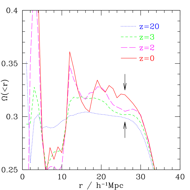
We will test NAM in a $N$-body simulation of a $\Lambda$CDM cosmology with matter density $\Omega_{\rm m}=0.3$, vacuum energy density $\Omega_{\rm\Lambda}=0.7$ (in units of the critical density $\rho_{\rm c}$), and a Hubble constant $h=0.7$ (in units of 100$\ {\rm km\,s^{-1}\,Mpc^{-1}}$). The simulation has an initial fluctuation power spectrum of spectral index $n=1$ and a present-day normalization amplitude $\sigma_{8}=0.9$. It was run with the GADGET $N$-body code (Springel, Yoshida & White 2001). It is part of a suite of simulations which zoom in on a spherical region of initial comoving radius 26$\ {\rm{\it h}^{-1}Mpc}$ selected from a larger parent simulation (see Stoehr 2003 for details). This “zooming” technique has the advantage of preserving the large-scale power of the parent simulation while allowing the inner region to be resolved at smaller scales. In particular, the mass of the 168436 “high-resolution” particles which sample the inner region is $m_{{}_{\rm HR}}=6.82\times 10^{10}\ {\rm M_{\odot}/{\it h}}$, in contrast to the 602272 “low-resolution” particles (each having a mass $\gg m_{{}_{\rm HR}}$) which sample the outer region.

Fig. 1 shows the average matter density $\Omega(<r)$ averaged over a sphere of radius $r$ as a function of redshift. At the initial time step ($z=20$), the mean density in a sphere of radius $r=26\ {\rm{\it h}^{-1}Mpc}$, $\Omega(<26)$, is very close to $\Omega_{\rm m}$, but increases by about 10 per cent from initial to final time. The net mass inflow across the region boundary has the potential to disrupt the reconstruction at the edge of the region and provides a further opportunity to test the sensitivity of NAM to the total mass.

Figure 2: The friends-of-friends differential mass function of dark matter haloes (in logarithmic bins $\Delta\log_{10}m=0.2$) computed from the snapshot at $z=0$ (histogram) compared to the theoretical prediction of Sheth & Tormen (dashed curve). The arrow indicates $M_{\star}\sim 10^{13}\ {\rm M_{\odot}/{\it h}}$, or the typical mass of haloes collapsing at the present time.

2.1 The halo catalogue

The principal objective of this paper is to test the ability of NAM to reconstruct the orbits of simulated dark matter (DM) haloes which resemble the galaxy + halo distributions of the “real world”. To this end we need to specify the positions, velocities and masses of a fixed number of haloes as a function of time, since our implementation of NAM conserves particle number. However, haloes do not form at any single redshift, and mergers potentially play an important role in the dynamics.

In order to create a catalogue of a fixed number of haloes from the inner region of the simulation, we first identify all the DM haloes above a given mass threshold $M_{\rm min}$ in the final simulation time step $z=0$, using a friends-of-friends (FOF) group-finding algorithm based on the method given in Davis et al. (1985). Only groups containing at least 20 DM particles are classified as haloes, resulting in a mass threshold $M_{\rm min}=1.36\times 10^{12}\ {\rm M_{\odot}/{\it h}}$. We used the standard linking length of 20 per cent of the mean interparticle distance (Jenkins et al. 2001). Using haloes defined with a linking length of 30 per cent we found a significant improvement in the accuracy of NAM reconstructions, which is not unexpected since this probes a more linear regime. In this paper however we confine our analysis to the standard linking length since it most closely reproduces the expected mass function and thus gives the best approximation to real galaxy haloes.

The center of mass (CM) positions and velocities of all those DM particles which are associated with haloes at $z=0$ define the resulting catalogue of 576 objects which is the input to the numerical action code. The orbit histories of these objects are then defined as the CM positions and velocities of the DM particles which belong to the corresponding halo at $z=0$. For our purposes the redshift outputs at $z$=20, 4, 3, 2, 1 and 0 were sufficient for comparison of halo orbits with the action reconstruction.

To model the tidal field from the outer region of the simulation, we created an auxiliary particle catalogue from a random sample of 1000 low-resolution DM particles, multiplying the masses by the appropriate factor of $277.9$ to bring the mass density in the outer region to $\Omega_{\rm m}=.3$. To reduce the computational burden, the positions of these tidal field particles were fixed in the NAM reconstructions and their masses were evolved according to linear perturbation theory, as described in Shaya et al. (1995). Parallel sets of NAM solutions were created with and without this tidal field.

The final step is to identify one of the haloes near the center of the simulation as the reference halo, and to build an input catalogue to NAM using the angular positions and redshifts relative to this halo. The analysis below was repeated for two haloes within 8 Mpc/h of the CM of the high-resolution region, as a check on the sensitivity to the position and velocity of the reference halo, and since the results were consistent we will confine our analysis to a single reference halo.

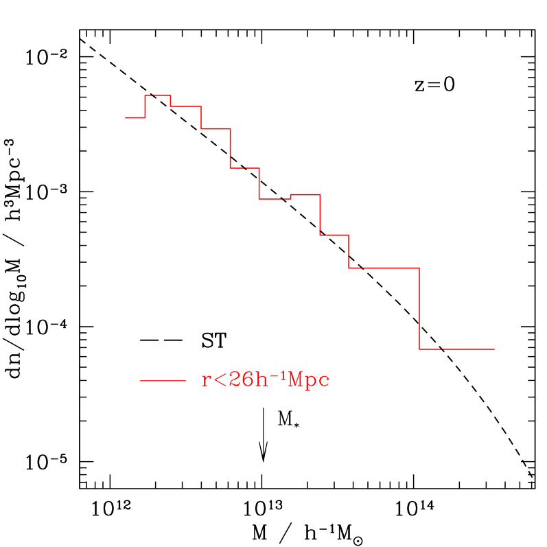
In Fig. 2 we show as a histogram the FOF differential mass function of DM haloes in the high-resolution region at $z=0$. The arrow marks $M_{\star}\sim 10^{13}\ {\rm M_{\odot}/{\it h}}$, the typical mass of haloes that have just formed by redshift $z=0$. As can be seen, the halo masses span more than two orders of magnitude, with the largest haloes having a mass $M~{}\hbox to0.0pt{$>$\hss}{\lower 4.30554pt\hbox{$\sim$}}10^{14}\ {\rm M_{\odot}/{\it h}}$. The dashed curve is the theoretical prediction of Sheth & Tormen (1999) for a $\Lambda$CDM cosmology matching that of the simulation. The good agreement shows that the high-resolution region of the simulation is a fair reproduction of the expected mass function.

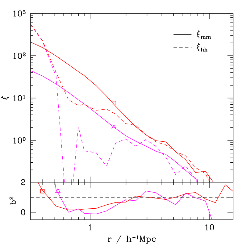
In the top panel of Fig. 3 we compare the auto-correlation of DM particles (solid) and haloes (dashed), $\xi_{{}_{\rm mm}}$ and $\xi_{{}_{\rm hh}}$ respectively. In the lower panel we plot the bias $b^{2}\equiv\xi_{{}_{\rm hh}}/\xi_{{}_{\rm mm}}$. The dotted horizontal line marks $b=1$. Results are shown at redshift $z=0$ (square) and 1 (triangle). Note that, on the scale $r~{}\hbox to0.0pt{$>$\hss}{\lower 4.30554pt\hbox{$\sim$}}2\ {\rm{\it h}^{-1}Mpc}$, DM haloes are as biased as the matter, i.e. $b\simeq 1$. This follows from the fact that at $z=0$ most of the haloes have a mass $M~{}\hbox to0.0pt{$<$\hss}{\lower 4.30554pt\hbox{$\sim$}}M_{\star}\approx 10^{13}\ {\rm M_{\odot}/{\it h}}$ (see Fig. 2), where $M_{\star}(z)$ is the typical mass of haloes which collapse at redshift $z$. The bias factor inferred from the unsmoothed $\xi_{{}_{\rm hh}}$ and $\xi_{{}_{\rm mm}}$ characterizes the clustering of DM haloes. We will propose below that it is possible using NAM to directly measure this bias factor when the total mass is known.

Figure 3: The auto-correlation of haloes (dashed curve) and dark matter (solid curve) obtained from the unsmoothed halo and matter distribution at $z=0$ (square) and $z=2$ (triangle). The bias $b^{2}=\xi_{{}_{\rm hh}}/\xi_{{}_{\rm mm}}$ is plotted in the lower panel. The horizontal dashed line shows $b=1$.

3 The action reconstruction

The implementation of NAM used in this paper is fully described in Peebles et al. (2001) and Phelps (2002). We refer the reader to appendix A for details. NAM solves for the orbits of mass tracers given the boundary conditions that the object positions in redshift space are fixed at the present time and that at the initial time $a^{2}m_{i}d{\mathbf{x_{i}}}/dt\rightarrow 0$. While some implementations of NAM expand the orbits in terms of suitable trial functions (Peebles 1989, 1990, 1994; Nusser & Branchini 2000), the present implementation relies on matrix inversion of a discrete form of the equations of motion (Peebles 1995, Phelps 2002), which allows the creation of more complex orbits. In this formulation the initial velocities $ad{\mathbf{x_{i}}}/dt$ are not mathematically constrained to vanish. Our approach to this problem will be discussed in the following section.

The generation of solutions begins with a set of randomized halo orbits with 10 time steps and relaxes to a target in the gradient of the action many orders of magnitude below that of the initial guess by iterated per-particle matrix inversion. Different choices of initial randomized orbits may yield different solutions, since uniqueness is not guaranteed, and so for each choice of cosmological parameters a suite of 8 solutions was generated and the solution with the lowest $\chi^{2}$ (see below) was used. Orbits with negative radial distances are allowed mathematically but in such cases the orbit is re-randomized and the matrix inversion procedure repeated until all of the particles have positive distances. The resulting orbit paths satisfy the standard equations of motion, as confirmed by a simple leapfrog integration forward in time from the first time step of the solution. Solutions with intersecting orbits, which are also mathematically allowed, are effectively suppressed by modelling each particle as a constant density sphere with radius proportional to the cube root of the mass, normalized so that a halo of mass $2.4\times 10^{11}\rm M_{\odot}$ has a radius of 180 kpc.

To more closely parallel the observational situation, where redshifts are known to greater accuracy than the distances, the standard action was recast with a partial transformation of coordinates, as described in Phelps 2002, so that the redshift at $z=0$ is fixed as the boundary condition instead of the radial distance. The distances then emerge as predictions, from which a standard $\chi^{2}$ measure is defined to measure the goodness of fit of the solutions:

$$\chi^{2}=\sum_{i}\frac{(\mu_{i}^{mod}-\mu_{i}^{cat})^{2}}{\sigma_{i}^{2}},$$ (1)

where $\mu_{i}^{mod}$ and $\mu_{i}^{cat}$ are the predicted and catalogue distance moduli for each particle and $\sigma_{i}$ is the dispersion in the observed distance moduli. Since there are no observational errors in the simulation, we added to the input distance moduli a gaussian random error with a dispersion of $\sigma_{i}=.2$ (10 per cent distance errors) when computing contours in $\chi^{2}$. As the mean $\chi^{2}$ may be dominated by a few particles with large distances errors that have settled on the wrong side of a triple-value zone, we exclude the ten highest per-particle $\chi^{2}$s in the computation of the mean. Excluding the tail of the distribution was found to affect the magnitude but not the location of the minimum $\chi^{2}$.

Since our goal is the comparison of predicted and actual halo orbits, it was useful to define two further quantitative measures of the quality of the orbits, the first, ${\overline{\Delta\theta}}$, the “directional error”, being defined as the per-particle average angle between the predicted and actual halo velocity vectors at $z=0$, and the second, ${\overline{\Delta d}}$, the “initial displacement error”, being the average per-particle distance between the actual and predicted halo positions at the first time step.

3.1 Halo mass assignment: background mass and linear growth factor

While each halo has a well-defined mass according to the FOF algorithm, the total mass in haloes is only 37 per cent of the total mass in the simulation catalogue. If each halo were simply assigned its bare FOF mass, then the mean density in the catalogue region as input to NAM would be too low, and in the NAM reconstruction the region would behave dynamically like a local void. Since the boundary condition in the action is the redshift, and since particles at a given distance would have higher redshifts in the reconstruction owing to the repulsive effect of the void, NAM would predict halo distances that are too small.

In observational catalogues, where the galaxy luminosities are given and where $\Omega_{\rm m}$ is assumed to be unknown, the standard approach is to multiply each galaxy by some constant factor, its mass to light ratio M/L, which may be a function of galaxy type. The minimum in $\chi^{2}$ as a function of M/L will then be governed by a combination of two factors: the degree to which the total mass in the catalogue region matches the background density set by $\Omega_{\rm m}$, and the gravitational dynamics of galaxies, groups and clusters. In practice the dominant contribution to $\chi^{2}$ is the former factor, which is largely independent of the dynamics of the haloes themselves.

In an $N$-body simulation we define the “halo mass multiplier” $\mathcal{M}$, the analogue of M/L in the observational catalogues, as the global factor by which we multiply the halo masses, which in our simulation gives a mass density of $\Omega_{\rm m}=.3$ when ${\mathcal{M}}=2.7$. Since $\Omega_{\rm m}$ is a known quantity, and since it is also known whether the region under study is close to the global mean density, it is possible in this case to employ NAM as a probe not only of the total mass but also of the relative distribution of mass in haloes relative to the background, i.e. the bias. We do this by simply adding a smooth constant density component to the value of $\Omega_{\rm m}$ which is input to NAM so that, for any choice of $\mathcal{M}$, the total mass density in the catalogue region is matched to the input $\Omega_{\rm m}$. When the total dark matter density in the catalogue region is close to the global mass density, as it is in our simulation, this is equivalent to multiplying $\Omega_{\rm m}$ as it appears in eq. A15 by the factor ${\mathcal{M}}/2.7$. When ${\mathcal{M}}=2.7$ the smooth component vanishes and all of the mass is located in the haloes as before. With this reassignment of the catalogue mass, a search for a minimum in $\chi^{2}$ in the space of $\mathcal{M}$ becomes a test of the linear bias relation between the underlying mass density and the halo distribution. To reiterate this important point: By assuming prior knowledge of $\Omega_{\rm m}$, we can use NAM to probe the relative distribution of dark matter in the haloes vs. the background. We will motivate this further in the following subsection.

A further modification to the halo masses is demanded by the absence of an analytical zero velocity constraint at the initial time step. Since in addition the haloes are modeled as non-evolving point masses throughout their histories, NAM solutions involving close interactions between haloes at high redshift are commonly seen. While we have not found a way, within the framework of the matrix inversion implementation of the action, to write down an analytical initial-time zero-velocity constraint, we have found that initial velocities are effectively suppressed by the procedure, already employed in modeling the tidal field, of rescaling the halo masses in time according to linear perturbation theory. We thus multiply the halo masses at each time step by the standard linear growth factor (see Peebles 1980, eq. 11.15), which is zero at $t=0$ and unity at $z=0$. The value of $\Omega_{\rm m}$ in eq. A15 is further rescaled by the same factor to maintain parity at each time step with the halo mass density. This ad hoc procedure forces the initial velocities to vanish, eliminates hard interactions at early times, and significantly reduces the nonuniqueness in the solutions, but at the cost of producing halo orbits with typical total displacements some 20 per cent shorter than the actual paths in the simulation. We conclude that there is room for improvement in our method of defining halo masses, and anticipate that some variation on the above theme, or the discovery of an analytical zero-velocity constraint, will open the way to further improvements in the reconstructions presented below.

3.2 Biasing and the mass to light ratio

Consider a discrete distribution of objects (haloes) sampling the underlying mass density field in a region of volume $V_{0}$ in the universe. Let $n({\bf x})$ be the number density of haloes and $\rho_{\rm m}({\bf x})$ be the mass density field, at comoving position ${\bf x}$. Denote the mean values of $n({\bf x})$ and $\rho_{\rm m}({\bf x})$ inside $V_{0}$ by $\overline{n}$ and ${\overline{\rho}}_{\rm m}$, respectively. Further, choose $V_{0}$ to be large enough such that ${\overline{\rho}}_{\rm m}$ is very close to the universal value $\Omega_{\rm m}\rho_{\rm c}$. Assume that the halo and DM density fields are related by means of a linear bias relation between the the density contrasts $\delta_{\rm h}({\bf x})=n({\bf x})/{\overline{n}}-1$ and $\delta_{\rm m}({\bf x})=\rho_{\rm m}({\bf x})/{\overline{\rho}}_{\rm m}-1$. We write this biasing relation as

$$\delta_{\rm h}=b\delta_{\rm m}\;.$$ (2)

We will express the bias factor $b$ in terms of the assumed $\mathcal{M}$ of haloes as it is invoked in the formalism of NAM presented here. This is useful in connecting this formalism to standard applications of the linear theory of gravitational instability as well as to other implementations of NAM (e.g. Nusser & Branchini 2000). A natural way to proceed is to use the Poisson equation and the bias relation (2) to write the peculiar acceleration, ${\bf g}$, of an object in terms of $\delta_{\rm h}$ and to compare that with the corresponding expression derived from NAM. The Poisson equation is

$${\bf\nabla}\cdot{\bf g}=-4\pi G{\overline{\rho}}_{\rm m}\delta_{\rm m}\;,$$ (3)

which upon integration and substituting $\delta_{\rm h}=b\delta_{\rm m}$ gives

$${\bf g}({\bf x})=-G{\overline{\rho}}_{\rm m}b^{-1}\int{\rm d}^{3}x^{\prime}\delta_{\rm h}({\bf x}^{\prime}){\bf K}({\bf x},{\bf x}^{\prime})$$ (4)

where ${\bf K}({\bf x},{\bf x}^{\prime})=({\bf x}-{{\bf x}}^{\prime})/|{\bf x}-{{\bf x}}^{\prime}|^{3}$. In discrete form,

$${\bf g}({\bf x})=-G\frac{{\overline{\rho}}_{\rm m}}{{\overline{n}}}b^{-1}\sum_{i}{\bf K}({\bf x},{\bf x}_{i})+\frac{4\pi}{3}G{\overline{\rho}}_{\rm m}{b}^{-1}{\bf x}$$ (5)

NAM gives, when $a=1$,

$${\bf g}_{\rm a}=-G\sum_{i}m_{i}{\bf K}({\bf x},{\bf x}_{i})+\frac{4\pi}{3}G{\overline{\rho}}_{\rm mc}{\bf x}$$ (6)

where $m_{i}$ is the mass assigned to object $i$ and ${\overline{\rho}}_{\rm mc}=\sum_{i}m_{i}/V_{0}$ is the mean mass density estimated from the objets. Define $m_{0i}$ such that for $m_{i}=m_{0i}$ we have ${\overline{\rho}}_{\rm mc}={\overline{\rho}}_{\rm m}$. In this case, a comparison between (5) and (6) implies $m_{0i}={\overline{\rho}}_{\rm m}/\overline{n}$ and $b=1$. Consider now ${\overline{\rho}}_{\rm mc}\neq{\overline{\rho}}_{\rm m}$. The difference between the mean mass densities must be attributed to a uniformly distributed mass component which can be associated with low (luminosity) objects that are not included in the catalogue. Low mass objects are typically less biased than higher mass ones (Mo & White 1996). Comparison between the uniform terms in (5) and (6) implies

$$b=\frac{{\overline{\rho}}_{\rm m}}{{\overline{\rho}}_{\rm mc}}\;,\quad{\rm and}\quad m_{i}=b^{-1}m_{0i}\;.$$ (7)

In most of the applications of NAM to real data, the masses $m_{i}$ are estimated from the luminosities, $L_{i}$, by $m_{i}={\mathcal{M}}L_{i}$ where $\mathcal{M}$ is a global mass to light ratio. Assume that ${\overline{\rho}}_{\rm mc}={\overline{\rho}}_{\rm m}$ is obtained for ${\mathcal{M}}={\mathcal{M}}_{0}$. Then, for a biased distribution of objects, the relations (7) imply that the same peculiar acceleration is obtained with the global mass to light ratio

$${\mathcal{M}}=b^{-1}{\mathcal{M}}_{0}\;.$$ (8)

In our simulation, since $b\simeq 1$ on the scale $r~{}\hbox to0.0pt{$>$\hss}{\lower 4.30554pt\hbox{$\sim$}}2\ {\rm{\it h}^{-1}Mpc}$ and since ${\mathcal{M}}_{0}=2.7$, we will expect to find the best solutions when ${\mathcal{M}}\simeq 2.7$, i.e. when all the mass is located in the haloes.

4 Results

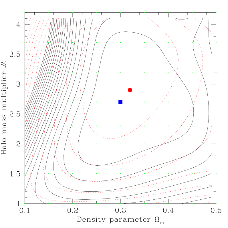
We searched for a minimum in $\chi^{2}$ in the two-dimensional parameter space of $\Omega_{\rm m}$ and $\mathcal{M}$, holding $H_{0}$ constant at 70, by finding NAM solutions on a grid of 56 points and interpolating a contour map in $\chi^{2}$. The results are shown in Fig. 4. At 1$\sigma$ the best solutions are found at $.27<\Omega_{\rm m}<.45$ and $1.7<{\mathcal{M}}<3.9$, consistent with the simulation parameter $\Omega_{\rm m}=.3$ and the predicted ${\mathcal{M}}=2.7$ (since $b\simeq 1$). A second set of solutions was computed without the external tidal field, and its absence had little effect on the quality of the solutions or the location of the minimum in $\chi^{2}$. In an idealized scenario where the exact halo masses are known, and where the region being reconstructed is a fair sample of the global mean, NAM can thus correctly recover both $\Omega_{\rm m}$ and $b$ but with an uncertainty of about 50 per cent in both values. In an actual observational situation with a comparable number of particles, where significant uncertainties in the galaxy + halo masses must additionally be taken into account, it is expected that the uncertainties in the predicted values of $\Omega_{\rm m}$ and $b$ will be even larger. It should be remarked that the tightness of these constraints is partially a function of the size of the catalogue, since $sigma$ in a standard $\chi^{2}$ measure is an inverse square-root function of the number of particles entering into the computation of $\chi^{2}$.

Figure 4: Mean $\chi^{2}$ contours showing the sensitivity of NAM to $\Omega_{\rm m}$ and, through $\mathcal{M}$, to the linear bias $b$. Solid contours lines are from solutions including the external tidal field and dotted contour lines are from a parallel set of solutions computed without the tidal field. Contour levels in both cases are .06 or $1\sigma$. The lowest computed mean $\chi^{2}$ of 1.3 (including the tidal field) was found at $\Omega_{\rm m}=.3$, ${\mathcal{M}}=2.7$ (corresponding to $b=1$). At each grid point a set of 16 solutions was computed, half with and half without the tidal field. For values of ${\mathcal{M}}$ different from 2.7 a smooth component is added to ensure that the total mass density in the catalog matches the background density. The filled square at center shows the global simulation parameters, assuming a linear bias of unity, and the nearby filled circle the parameters in the catalog region, which is slightly overdense due to mass inflow across the catalog boundary.

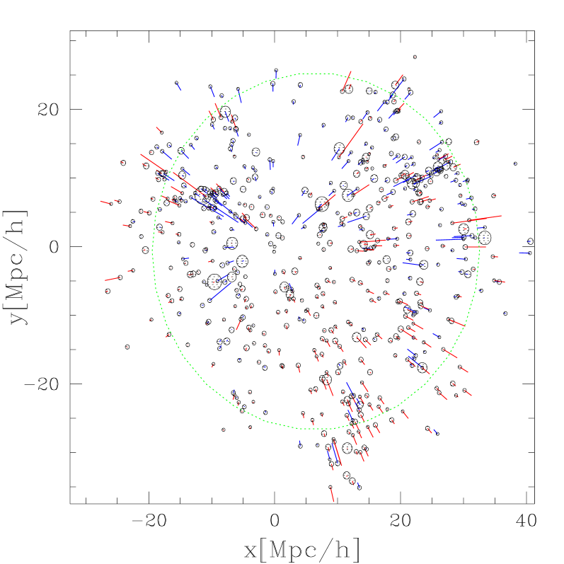
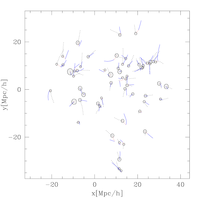
A series of closer looks at the best obtainable NAM solution (Figs. 5 through 9), all plotted from the same solution with input parameters $\Omega_{\rm m}=.3$, ${\mathcal{M}}=2.7$, gives a good feel for the strengths and limitations of the method. Note that for this solution all of the mass is located within the haloes. Fig. 5 shows in x-y projection the final positions of the haloes in the high-density region of the simulation (open circles, with radii proportional to the mass) and the error in the predicted positions (line segments). Note that the distance errors are purely radial due to the boundary condition in the action. The reconstruction tends to be less accurate in the vicinity of massive haloes, which is due to the presence of triple-value regions where NAM is easily confused.

Figure 5: catalogue vs. predicted halo positions at $z=0$ in x-y projection, for the best case solution at $\Omega_{\rm m}=.3$, ${\mathcal{M}}=3.2$. The dotted outer circle (in green) marks the nominal $26\ {\rm{\it h}^{-1}Mpc}$ boundary of the high-density region of the simulation. Actual halo positions at the final time step are marked by circles with radii proportional to $m_{i}^{1/3}$. The free end of the line segments mark the positions predicted by NAM (red when the predicted distances are larger and blue when they are smaller); the length of the line segment thus reveals the radial distance error.

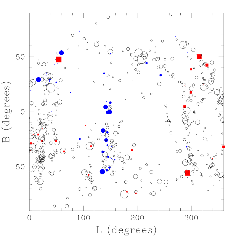
This can be seen more clearly in Fig. 6, which shows a view of the “sky” from the reference halo, highlighting those haloes with the largest $\chi^{2}$. Some of these haloes are found near the edge of the catalog region, where interactions with particles in the low-resolution region, which is only approximately modelled by NAM, may disrupt the reconstruction. The majority of the remaining haloes with high $\chi^{2}$ are often found within a few degrees of the line of sight to a massive halo; these have typically settled on the wrong side of a triple-value region. Haloes with high $\chi^{2}$ also tend to be found close to each other, suggesting that if the dynamics of one influential halo are not correctly modelled it may disrupt the accurate reconstruction of several other nearby haloes. Finally, a few small haloes with large distances errors can be seen in relative isolation, indicating that the interaction of haloes with unassociated dark matter particles, and the complex formation and merger history of the haloes themselves, may prevent accurate NAM reconstruction even in the absence of more obvious disruptive factors.

Figure 6: A view of the “sky” from the perspective of the reference halo near the center of the simulation, highlighting the location of haloes with poorly recovered distances in the best NAM solution. Point size is proportional to the halo mass. Filled points indicate haloes with $\chi^{2}>1$ (radial distance error greater than 10 per cent). For haloes located towards the edge of the catalogue ($>24Mpc/h$) these are indicated by filled squares, and towards the center of the catalogue ($<24Mpc/h$), by filled circles.

The top panel of Fig. 7 shows the error in the predicted distances as a function of the distance from the reference halo. Here the excellent overall prediction of halo distances, with typical errors of less than 3 per cent, can be seen most clearly. Any mismatch in the halo mass density relative to $\Omega_{\rm m}$ would be revealed here by a tilt in the distance errors as a function of distance from the reference halo (with a positive slope indicating an overdensity and a negative slope an underdensity). As the distance errors trace a line with vanishing slope, this confirms that the total mass for a choice of ${\mathcal{M}}=2.7$ is well matched to $\Omega_{\rm m}$. The bottom panel of Fig. 7 compares the distance errors with those obtained assuming zero peculiar velocities and Hubble-flow distances ($d=cz_{i}H_{0}$). In the latter case the average distance errors are 5 per cent. The difference in the sharpness of the peaks in the two histograms gives an indication of the ability of NAM to correctly model the interparticle dynamics.

Figure 7: Top panel : Scatterplot of the error in radial distance predictions for the best NAM solution, showing good overall recovery of the distances. Point size is proportional to halo mass. Bottom panel : Histogram in $\chi\equiv(\mu_{i}^{mod}-\mu_{i}^{cat})/\sigma_{i}$ of the same solution. For comparison the dotted line shows the errors obtained when Hubble-flow distances are used in place of $\mu_{i}^{cat}$.

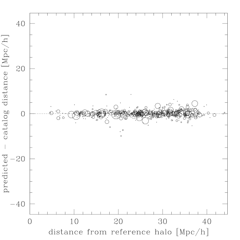
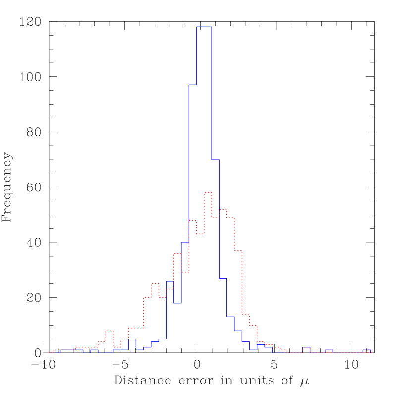
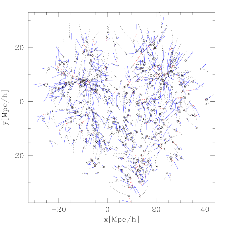
Fig. 8 compares the NAM-reconstructed halo orbits with the actual halo orbits, the latter being defined previously as the CM motion of the dark matter particles comprising the halo at $z=0$. The reconstruction is more accurate for the heaviest haloes (top panel) than for the rest (bottom panel): for the former the directional error $\overline{\Delta\theta}=41^{o}$, while for the latter $\overline{\Delta\theta}=48^{o}$. By comparison, the chance that a random orbit will have a directional error of $48^{o}$ or less, that is, that a point placed at random within a sphere will fall within the volume of the cone swept out by an opening angle of $2*48^{o}$, is about 17 per cent. According to the directional error the quality of the orbit reconstructions, like $\chi^{2}$, is not a particularly sensitive function of ${\mathcal{M}}$: far from the $\chi^{2}$ minimum at the same $\Omega_{\rm m}$ and ${\mathcal{M}}=1$, $\overline{\Delta\theta_{i}}\simeq 50^{o}$ for the entire catalogue. Similarly, the average initial displacement error $\overline{\Delta d_{i}}$, was 2.5 Mpc/h for the best solution at ${\mathcal{M}}=2.7$ , while far from the minimum at ${\mathcal{M}}=1$ it was 2.9 Mpc/h. A further indication of the approximate character of the predicted orbits is that the magnitude of the initial displacement error is comparable to the total distance travelled by the typical halo orbit: The centre of mass of the average halo in the simulation travelled 3.2 Mpc/h, while the reconstructed haloes travelled an average of 2.6 Mpc/h, the shorter path lengths in the reconstruction being a feature of our halo mass assignment scheme as discussed in section 3.1. While this error may seem large, the chance that a random orbit with a total displacement of 2.6 Mpc/h will end up within 2.5 Mpc/h of the actual initial position is only 16 per cent (this is the volume overlap of two spheres of equal radii whose centers are separated by a distance equal to their radii). A trial NAM reconstruction without the linear growth factor, assigning the full halo mass at early times, gave similar values for the late-time measures $\chi^{2}$ and $\overline{\Delta\theta_{i}}$, while the early-time measure $\overline{\Delta d_{i}}\sim 4.9Mpc/h$, or about twice the error. The average total distance travelled by the haloes in these solutions was 6.3 Mpc/h, nearly twice as long as the actual halo paths and illustrative of the instability of the solutions when the haloes are allowed to keep their full masses in the initial time steps.

Figure 8: x-y projection of actual (solid lines) and reconstructed orbits (dotted lines) for the heaviest haloes (top panel) and for all other haloes (bottom panel). Dotted lines indicate the actual halo paths to $z=20$, while solid lines mark the paths predicted by NAM. Actual halo positions are indicated by circles of radii proportional to the halo mass. Straight radial dotted line segments connect these positions to those predicted by NAM, as in Fig. 5. Heavier haloes tend to have more accurately reconstructed orbits: For the heaviest haloes $\overline{\Delta\theta_{i}}=41^{o}$ and for the remaining haloes $\overline{\Delta\theta_{i}}=48^{o}$.

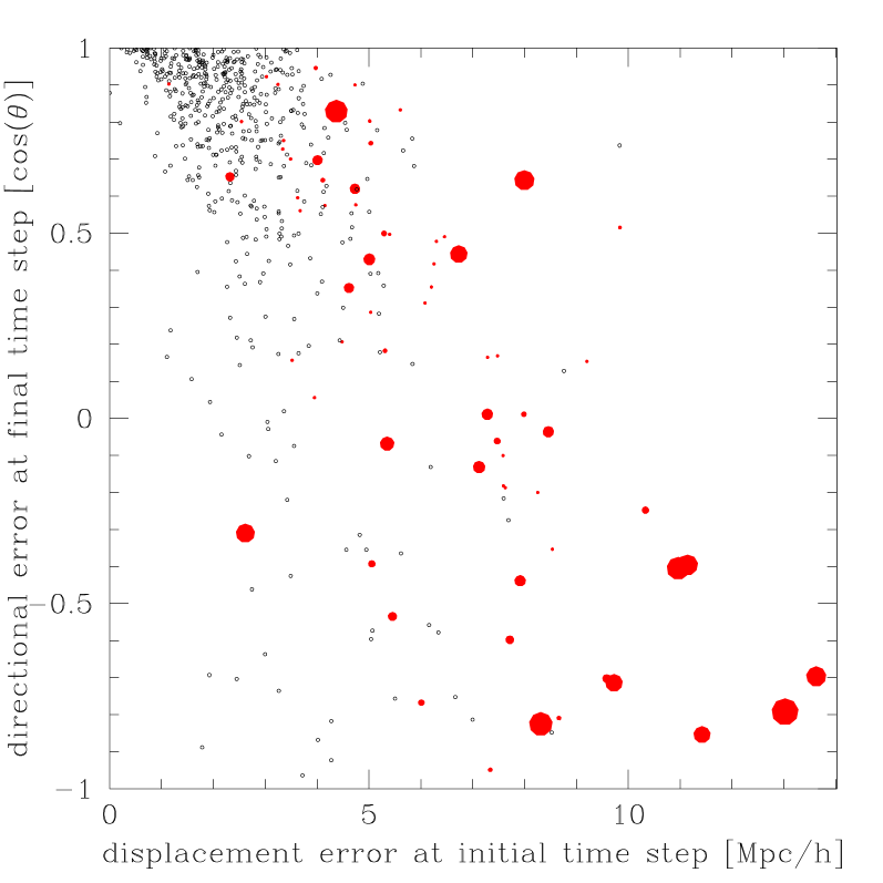
Finally, Fig. 9 compares three measures of errors in NAM reconstructions: $\overline{\Delta d_{i}}$ and $\overline{\Delta\theta_{i}}$ are plotted on the x and y axes, respectively, while the point size is proportional to $\chi^{2}$. Haloes with $\chi^{2}>1$ are shown as filled circles. $\chi^{2}$ is fairly well correlated to $\overline{\Delta d_{i}}$, indicating that reconstructed orbits which begin at positions well removed from their actual starting positions in the simulation are likely to end with inaccurately modeled distances. Significantly, $\chi^{2}$ is poorly correlated to $\overline{\Delta\theta_{i}}$. This may have been expected since, in the absence of nearby haloes constraining the dynamics, the motion of a given halo in the plane of the sky relative to the reference halo should be fully degenerate. The extent to which this degeneracy is broken and the transverse orbital motions at the present epoch are correctly recovered is a measure of the sensitivity of NAM to the dynamics between haloes. The weak correlation between $\chi^{2}$ and $\overline{\Delta\theta_{i}}$ is the clearest evidence that the predicted halo distances alone are not a sufficient discriminator of the quality of reconstructed orbits.

Figure 9: Scatterplot showing errors in the direction of the reconstructed final-time velocities, as well as errors in the early and late time predicted positions, for each of the 533 particles in the best NAM solution. The x-axis shows $\overline{\Delta d_{i}}$, the error in the initial placement of the haloes at the first timestep. The y-axis shows $\overline{\Delta\theta_{i}}$, the error in the direction of the velocity vector at the final timestep. Halo orbits which most accurately predict the direction of the halo orbit at the present epoch are thus found at the top of the graph. Point size is proportional $\chi^{2}$.

5 Discussion and conclusions

We have shown, using a catalogue of over 500 dark matter haloes derived from a large $N$-body simulation at the scale of the local supercluster, that it is possible with the numerical action method to reconstruct the full dynamical histories of dark matter haloes given the masses and the redshift space coordinates at the present epoch. The reconstruction is most successful in recovering the halo distances at the present epoch, with typical errors of less than 3 per cent. Individual orbits paths, including the initial positions as well as the direction of motion of the haloes at the present epoch, are predicted with less accuracy. By varying the relative contributions to the total mass from the haloes and the background, we have also found a way to use NAM to directly measure the linear bias when the total mass density is known, although with an uncertainty of about 50 per cent.

Given the dynamical complexity of millions of interacting particles, and the sweeping nature of NAM’s central simplifying assumption that galaxy haloes can be approximated as discrete, non-merging point masses throughout their evolution, it is remarkable how successfully the dynamics of a many-body system can be reconstructed on the basis of an incomplete catalogue of facts. The successes of NAM as it has been implemented here are of course partially offset by their weaknesses. Among these is the relatively poor quality of the reconstruction in the vicinity of massive haloes, clearly seen in Fig. 5, which shows a breakdown in the non-linear regime where NAM, which is itself a fully non-linear method, might have potentially offered the most insight. In these regions $\chi^{2}$ is a good indicator of poorly reconstructed orbits, but preliminary attempts to use this information to nudge haloes into the correct orbits while not imposing any additional formal constraints have so far been unsuccessful. A second concern is the inability of NAM in many cases to isolate, on the basis of $\chi^{2}$ alone, predicted halo orbits which are moving in the wrong direction at the present epoch. Fig. 9 shows, for example, 34 haloes moving more than $90^{o}$ in the wrong direction but with good distances at the present epoch and thus low $\chi^{2}$.

The above innacuracies may in part arise from the details of our implementation, such as our ad hoc procedure of scaling of halo masses according to linear theory, and there is certainly room here for improvement. The scale of the catalog is also a factor to consider, and in particlar the density of mass tracers within it. This analysis should be repeated at the scale of the Local Group, where a larger number of mass tracers acting within a smaller volume may better constrain the dynamics and permit more accurate orbit reconstructions. It is also possible that, in dynamical systems of this complexity, the angular positions, redshifts and masses are by themselves insufficient to lift the degeneracies in the halo orbits, and that the full three-dimensional velocities at the present epoch will be needed to accomplish this. This again is work to be undertaken at Local Group scales, where next-generation observations from SIM and GAIA hold out the promise of multiple galaxy proper motion measurements with which to test the NAM predictions. One related concern is that part of the proper motion data may be needed to recover accurate orbits, leaving fewer remaining free parameters to assist with the more weighty problem of constraining individual galaxy halo masses, although it is possible that only one of the two components of the tangential velocity will be sufficient to break the orbtial degeneracy. Finally, inaccuracies in the NAM predictions are doubtless due at least in part to intrinsic limitations of the method and its assumptions, although we do not wish to suggest at this stage, given the work that remains to be done, that that an upper limit on NAM accuracy in orbit reconstruction has yet been reached.

We anticipate that work on NAM in the near term will lie principally in two directions. The first is an extension of the above analysis, with further improvements in the implementation, to a high-resolution simulation at the scale of the Local Group, where present-day three-dimensional velocities can provide significant additional dynamical constraints. The second is a direct comparison of NAM with other reconstruction methods, both in real space (e.g, Nusser & Dekel 1992, Gramman 1993, Croft & Gaztañaga 1998, Frisch et al. 2002, Mohayaee et al. 2005) and redshift space (e.g., Narayanan & Weinberg 1998, Monaco & Efstathiou 1999, Mohayaee & Tully 2005), that help to bridge the present-day observations of large-scale structure with the initial conditions prevailing in the early universe.

We acknowledge the support of the Asher Space Research Institute. We would like to thank Felix Stoehr for providing us with the snapshots from his simulation.

Appendix A The cosmological action

The standard cosmological action in an expanding coordinate system, following Peebles (1989), is

$$\mathcal{S} = \int_{0}^{t_{0}}dt\left(\sum\frac{m_{i}a(t)^{2}}{2}\left(\frac{d\mathbf{x_{i}}}{dt}\right)^{2}\right.$$ (9)

$$\left.+\frac{G}{a}\sum\frac{m_{i}m_{j}}{\mid\mathbf{x_{i}}-\mathbf{x_{j}}\mid}\right.$$

$$\left.-\frac{2}{3}\pi G\rho(t)a(t)^{2}\sum m_{i}\mathbf{x_{i}}^{2}\right),$$

where $\mathbf{x_{i}}(t)$ are the co-moving coordinates, a(t) is the cosmological scale factor, and $\rho(t)$ is the mean background mass density.

The variation in the action, after integration by parts, is

$$\delta\mathcal{S} = \int_{0}^{t_{0}}{\rm d}t\,\delta{\bf x}_{i}\left[-\frac{{\rm d}}{{\rm d}t}m_{i}a^{2}\frac{{\rm d}{\bf x}_{i}}{dt}+m_{i}a{\bf g}_{i}\right]$$ (10)

$$+\,\left[m_{i}a^{2}\delta{\bf x}_{i}\frac{{\rm d}{\bf x}_{i}}{{\rm d}t}\right]^{t_{0}}_{0}=0,$$

where

$${\bf g}_{i}=\frac{G}{a^{2}}\sum_{j\neq i}m_{j}\frac{{\bf x}_{j}-{\bf x}_{i}}{|{\bf x}_{j}-{\bf x}_{i}|^{3}}+\frac{4}{3}\pi G\rho a{\bf x}_{i}.$$ (11)

The usefulness of the action in a cosmological context hinges upon the observation that the boundary term in (10) vanishes either when $\delta{\bf x}_{i}=0$ or $a^{2}{\rm d}{\bf x}_{i}/{\rm d}t=0$. The former condition obtains when all three position coordinates at $t_{0}$ are fixed. The latter condition is met automatically because $a=0$ at $t=0$.

Since cosmological redshifts can be more accurately measured than distances, however, it is desirable to find a way to fix the observed redshifts as a boundary condition in the action and leave the distances as free parameters, while leaving the angular position coordinates unchanged. The procedure can be transparently carried out in the Hamiltonian formulation of the action, where the independent status of generalized coordinates $q$ and momenta $p$ can be exploited:

$$\delta{\mathcal{S}}=\delta\int^{t_{0}}_{0}dt\left(\sum_{i}p_{i}\dot{q}_{i}-H(q_{i},p_{i})\right)=0.$$ (12)

As described fully in Phelps (2002), the coordinate transformation which exchanges the roles of the radial velocities and radial distances is carried out by adding a generating function to the Hamiltonian of the form

$$F=q^{r}p^{r}.$$ (13)

where the superscript $r$ refers to the radial component.

The modified action is

$${\mathcal{S}}=\sum_{i}\int\left(\vec{p}_{i}\cdot d\vec{q}_{i}-\frac{p_{i}^{2}}{2m}dt-V_{i}dt\right)-p_{i}^{r}q_{i}^{r}.$$ (14)

All boundary terms are evaluated at $t=t_{0}$, and

$$V_{i}=-\sum_{i\neq j}\frac{Gm_{i}m_{j}}{q_{ij}}-\sum_{i}\frac{\Lambda q_{i}^{2}}{6}.$$ (15)

The subscripts $i$ and $j$ will refer to the particle index, while superscripts will refer to coordinate indices.

In a homogeneous expanding coordinate system with scale factor $a(t)$, the physical position is

$$a\vec{x}$$ (16)

and the physical momentum is

$$m\dot{a\vec{x}}=\frac{\vec{p}}{a}+m\dot{a}\vec{x},$$ (17)

where $\vec{x}$ is the coordinate position and where we have redefined the variable $\vec{p}\equiv ma^{2}\dot{\vec{x}}$. Omitting for the moment individual particle subscripts, the action is then

$${\mathcal{S}} = \int\left[(\frac{\vec{p}}{a}+m\dot{a}\vec{x})\cdot(ad\vec{x}+\dot{a}\vec{x}dt)\right.$$ (19)

$$\left.-dt\left(\frac{\vec{p}^{2}}{2ma^{2}}+\frac{\dot{a}}{a}\vec{p}\cdot\vec{x}+\frac{m}{2}\dot{a}^{2}x^{2}+V\right)\right]$$

$$\mbox{}-\left(\frac{p^{r}}{a_{0}}+m\dot{a}_{0}x^{r}\right)a_{0}x^{r}$$

$$= \int\left[\vec{p}\cdot d\vec{x}+ma\dot{a}\vec{x}\cdot d\vec{x}+\frac{m}{2}\dot{a}^{2}x^{2}dt\right.$$

$$\left.-dt\left(\frac{p^{2}}{2ma^{2}}+V\right)\right]$$

$$\mbox{}-p^{r}x^{r}-m(x^{r})^{2}\dot{a}_{0}a_{0}.$$

After integration by parts, and substituting the standard pressureless form of the acceleration of the cosmological expansion,

$$\frac{\ddot{a}}{a}=-\frac{4}{3}\pi G\rho+\frac{\Lambda}{3},$$ (20)

the action can be written as

$${\mathcal{S}}=\int\left[\vec{p}\cdot d\vec{x}-\left(\frac{\vec{p}^{2}}{2ma^{2}}+\tilde{V}\right)dt\right]$$

$$-p^{r}x^{r}-\frac{m(x^{r})^{2}a_{0}\dot{a}_{0}}{2},$$ (21)

where $\tilde{V}$ is the gravitational potential modified by a smoothly distributed homogeneous background density,

$$\tilde{V}_{i} = -\sum_{j\neq i}\frac{Gm_{i}m_{j}}{ax_{ij}}+\frac{2}{3}\pi G\rho a^{2}m_{i}x_{i}^{2}$$ (22)

$$= -\sum_{j\neq i}\frac{Gm_{i}m_{j}}{ax_{ij}}+\frac{\Omega_{\rm m}H_{0}^{2}}{4a}a^{2}m_{i}x_{i}^{2}.$$ (23)

The cosmological constant is no longer explicitly found in the action, as expected since it cannot produce peculiar accelerations in co-moving coordinates. Its influence is felt in the timescale of the integration.

The action has thus been put in the standard Hamiltonian form, with conjugate variables $\vec{x}$ and $\vec{p}$, and with the addition of extra terms outside the integral, the first representing the generating function of the canonical transformation, and the second arising from the change of boundary conditions (for further details see Phelps 2002).

To recover the correct equations of motion, these boundary terms must vanish in the variational derivatives, and so the constraint which was implicit in the transformed coordinate system – that the final-time velocity of each particle relative to the origin is equal to its observed redshift – must be imposed by hand in the original coordinates. As the origin of the coordinate system is typically taken to be the Milky Way, its motion along the line of sight must be subtracted out:

$$v_{pec}+H_{0}r-\vec{v}_{0}\cdot\hat{x} = z,$$

$$\frac{p^{r}}{ma_{0}^{2}}+\frac{\dot{a}_{0}x^{r}}{a_{0}}-\vec{v}_{0}\cdot\hat{x} = z,$$ (24)

where $\vec{v}_{0}$ is the coordinate velocity of the Milky Way.

With the equation of constraint (A15), the action is written

$${\mathcal{S}}=\frac{m}{2}a_{0}\dot{a}_{0}(x^{r})^{2}-ma_{0}zx^{r}+ma_{0}^{2}x^{r}\vec{v}_{0}\cdot\hat{x}$$

$$\mbox{}+\int\left(\vec{p}\cdot d\vec{x}-\mathcal{H}dt\right).$$ (25)

By construction, solutions found by minimizing this modified action will contain particle orbits whose final time-step angular positions and radial velocities relative to the reference particle will equal the input angular positions and redshifts. Distances and transverse velocities at $z=0$, as well as the orbit history of each particle, emerge as predictions.

The rest of the problem is in principle a computational one, and consists in devising a numerical approach to finding solutions to the variational integral. The first numerical applications of the action method used a set of fitting functions to characterize the orbits, and the action was minimized with respect to the coefficients of these functions. The procedure employed here follows Peebles (1995), where the positions are independent at each time step, allowing for the creation of sharper orbits.

In this implementation the $\alpha^{th}$ position coordinate of the $i^{th}$ particle at the $n^{th}$ time step is written as $x^{\alpha}_{i\>n}$. If there are $N$ time steps, then $x^{\alpha}_{i\>N+1}$ is defined to represent the present-time positions (the final time step is treated differently from the others, due to the boundary conditions). Time increments are defined every half step, so that $a=1$ at $t_{2N+1}$ (“$t_{0}$”) and $a=0$ at the first time step. The momentum is then defined, as in a standard leapfrog integration, at the half-steps, as $p^{\alpha}_{i\>2n}$. With this notation the action integral becomes a sum and the per-particle action is written as

$${\mathcal{S}}_{i} = \frac{m_{i}}{2}\dot{a}_{2N+1}(x^{r}_{i\>N+1})^{2}-m_{i}x^{r}_{i\>N+1}z$$ (26)

$$+m_{i}x^{r}_{i\>N+1}\vec{v}_{0\>N+1}\cdot\hat{x}_{i\>N+1}$$

$$+\sum_{n=1}^{N}\left[p^{\alpha}_{i\>2n}(x^{\alpha}_{i\>n+1}-x^{\alpha}_{i\>n})\right]$$

$$-\sum_{n=1}^{N}\left[\frac{(p^{\alpha}_{i\>2n})^{2}}{2m_{i}a^{2}_{2n}}(t_{2n+1}-t_{2n-1})\right.$$

$$\left.+\tilde{V}_{n}(t_{2n+1}-t_{2n-1})\right],$$

where the gravitational potential $\tilde{V}$ is defined as in equation (23).

The condition that the action be stationary with respect to the $p$-derivative yields an expression for $p^{\alpha}_{i\>2n}$ in terms of $x$ and $t$:

$$\frac{\partial{\mathcal{S}}_{i}}{\partial p^{\alpha}_{i\>2n}}=x^{\alpha}_{i\>n+1}-x^{\alpha}_{i\>n}-\frac{p^{\alpha}_{i\>2n}}{m_{i}a^{2}_{2n}}(t_{2n+1}-t_{2n-1})=0,$$ (27)

$$p^{\alpha}_{i\>2n}=\frac{m_{i}a^{2}_{2n}(x^{\alpha}_{i\>n+1}-x^{\alpha}_{i\>n})}{t_{2n+1}-t_{2n-1}}.$$ (28)

This is substituted back into the action, which is then expressed solely as a function of $x$:

$${\mathcal{S}}_{i} = \frac{m_{i}}{2}\dot{a}_{2N+1}(x^{r}_{i\>N+1})^{2}-m_{i}x^{r}_{i\>N+1}z$$ (29)

$$+m_{i}x^{r}_{i\>N+1}\vec{v}_{0\>N+1}\cdot\hat{x}_{i\>N+1}$$

$$+\sum_{n=1}^{N}\left[\frac{m_{i}a^{2}_{2n}}{2}\frac{(x^{\alpha}_{i\>n+1}-x^{\alpha}_{i\>n})^{2}}{t_{2n+1}-t_{2n-1}}\right.$$

$$\left.-\tilde{V}_{n}(t_{2n+1}-t_{2n-1})\right].$$

To find stationary points in the action through matrix inversion, by means of the iterative approach described in Peebles (1995), the first and second derivatives of the action with respect to the position variables at each time step must be computed. Calculation of the derivatives is considerably simplified by fixing the orbits of all particles except the one whose orbit is being solved, as the off-diagonal terms can be ignored. The derivatives at the final time step are computed separately.

The gradient of the action for all time steps except the last is:

$$\frac{\partial{\mathcal{S}}_{i}}{\partial x^{\alpha}_{i\>n}} = m_{i}a_{2n-2}^{2}\frac{(x^{\alpha}_{i\>n}-x^{\alpha}_{i\>n-1})}{t_{2n-1}-t_{2n-3}}$$

$$-m_{i}a_{2n}^{2}\frac{(x^{\alpha}_{i\>n+1}-x^{\alpha}_{i\>n})}{t_{2n+1}-t_{2n-1}}-({t_{2n}-t_{2n-2}})\frac{\partial\tilde{V}_{n}}{\partial x^{\alpha}_{i\>n}}$$ (30)

and the second derivatives are

$$\frac{\partial^{2}{\mathcal{S}}_{i}}{\partial x^{\alpha}_{i\>n}\partial x^{\beta}_{i\>n}} = m_{i}\delta^{\alpha\beta}\left(\frac{a_{2n}^{2}}{t_{2n+1}-t_{2n-1}}\right.$$

$$\left.+\frac{a_{2n-2}^{2}}{t_{2n-1}-t_{2n-3}}\right)-(t_{2n}-t_{2n-2})\frac{\partial^{2}\tilde{V}_{n}}{\partial x^{\alpha}_{i\>n}\partial x^{\beta}_{i\>n}}$$ (31)

for the same time step, and

$$\frac{\partial^{2}{\mathcal{S}}_{i}}{\partial x^{\alpha}_{i\>n}\partial x^{\alpha}_{i\>n+1}}=-\frac{m_{i}a_{2n}^{2}}{t_{2n+1}-t_{2n-1}}$$ (32)

for different time steps.

The gradient and second derivatives of the potential are

$$-\frac{\partial\tilde{V}_{n}}{\partial x^{\alpha}_{i\>n}} = \sum_{j\neq i}\frac{Gm_{i}m_{j}}{a_{2n-1}}\frac{x^{\alpha}_{ji\>n}}{x^{3}_{ji\>n}}$$

$$+\frac{H_{0}^{2}\Omega_{\rm m}}{2a_{2n-1}}m_{i}x^{\alpha}_{i\>n}$$ (33)

$$-\frac{\partial^{2}\tilde{V}_{n}}{\partial x^{\alpha}_{i\>n}\partial x^{\beta}_{i\>n}}=\sum_{j\neq i}\frac{Gm_{i}m_{j}}{a_{2n-1}}\left[\frac{\delta^{\alpha\beta}}{{x^{3}_{ji\>n}}}\right.$$ (34)

$$\left.-3\frac{x^{\alpha}_{ji\>n}x^{\beta}_{ji\>n}}{x^{5}_{ji\>n}}\right]+\frac{H_{0}^{2}\Omega_{\rm m}}{2a_{2n-1}}m_{i}\delta^{\alpha\beta}.$$

At the final time step, when $i\neq 1$, only the components of the gradient in the radial direction are needed:

$$\frac{\partial{\mathcal{S}}_{i}}{\partial x^{r}_{i\>N+1}}=m_{i}(H_{0}x^{r}_{i\>N+1}-z+\vec{v}_{0\>N+1}\cdot\hat{x}^{\alpha}_{i\>N+1})$$ (35)

$$+\sum_{\alpha}m_{i}a_{2N}^{2}\frac{\hat{x}^{\alpha}_{i\>N+1}\cdot(x^{\alpha}_{i\>N+1}-x^{\alpha}_{i\>N})}{t_{2N+1}-t_{2N-1}}$$

$$-\sum_{\alpha}({t_{2N+1}-t_{2N}})\frac{\partial\tilde{V}_{N+1}}{\partial x^{\alpha}_{i\>N+1}}\cdot\hat{x}^{\alpha}_{i\>N+1},$$

where $\hat{x}_{i\>N+1}$ is referred to the origin and so is purely radial.

The second derivatives are

$$\frac{\partial^{2}{\mathcal{S}}_{i}}{\partial x^{r}_{i\>N+1}\partial x^{r}_{i\>N+1}}=m_{i}H_{0}+\frac{m_{i}a_{2N}^{2}}{t_{2N+1}-t_{2N-1}}$$ (36)

$$-\sum_{\alpha}\sum_{\beta}(t_{2N+1}-t_{2N})\frac{\partial^{2}\tilde{V}_{N+1}}{\partial x^{\alpha}_{i\>N+1}{\partial x^{\beta}_{i\>N+1}}}$$

$$\cdot\hat{x}^{\alpha}_{i\>N+1}\cdot\hat{x}^{\beta}_{i\>N+1}$$

for the same time step, and

$$\frac{\partial^{2}{\mathcal{S}}_{i}}{\partial x^{\alpha}_{i\>N}\partial x^{\alpha}_{i\>N+1}}=-\frac{m_{i}a_{2N}^{2}\hat{x}^{\alpha}_{i\>N+1}}{t_{2N+1}-t_{2N-1}}$$ (37)

for the last two time steps.

References

- [1] Branchini E., Carlberg R. G., 1994, ApJ, 434, 37
- [2] Branchini E., Eldar A., Nusser A., 2002, MNRAS, 335, 53
- [3] Croft R. A. C., Gaztanaga E., 1998, ApJ, 495:554
- [4] Davis M., Efstathiou G., Frenk C.S., White S.D.M., 1985, ApJ, 292, 371
- [5] Dunn, A.M. and LaFlamme, R., 2005, ApJ, 443, 1.
- [6] Frisch U., Matarrese S., Mohayaee R., Sobolevskii A., 2002, Nature, 417, 260
- [7] Gramman, M., 1993, ApJ, 405, 449
- [8] Jenkins A., Frenk C.S., White S.D.M.,Colberg J.M., Cole S., Evrard A.E., Couchman H.P.M., Yoshida N., 2001, MNRAS, 321, 372
- [9] Kauffmann G., Nusser A., Steinmetz M., 1997, MNRAS, 286, 795
- [10] Mohayaee R., Mathis H., Colombi S., Silk J., 2005, MNRAS in press, astro-ph/0501217
- [11] Mohayaee R., Tully R.B., ApJL in press, astro-ph/0509313
- [12] Mo H.J., White S.D.M., 1996, MNRAS, 282, 347
- [13] Monaco P., Efstathiou G., 1999, MNRAS, 308, 763
- [14] Narayanan V.K., Weinberg D.H., 1998, ApJ, 508, 440
- [15] Nusser A., Dekel A., 1992, ApJ, 391, 443
- [16] Nusser A., Branchini E., 2000, MNRAS, 313, 587
- [17] Peebles P.J.E., 1980, The Large-Scale Structure of the Universe (Princeton University Press)
- [18] Peebles P.J.E., 1989, ApJ, 344, L53
- [19] Peebles P.J.E., 1990, ApJ, 362, 1
- [20] Peebles P.J.E., 1994, ApJ, 429, 43
- [21] Peebles P.J.E., 1995, ApJ, 449, 52
- [22] Peebles P.J.E., 1996, ApJ, 473, 42
- [23] Peebles P.J.E., Phelps S.D., Shaya E.J., Tully R.B., 2001, ApJ, 553, 2431
- [24] Phelps S.D., 2002, ApJ, 575, 1
- [25] Sharpe J. et al. , 2001, MNRAS, 322, 121
- [26] Shaya E.J., Peebles P.J.E., Tully R.B., 1995, ApJ, 454,15
- [27] Sheth R., Tormen G., 1999, MNRAS, 308, 119
- [28] Springel V., Yoshida N., White S.D.M., 2001, New Astronomy, 6, 79
- [29] Stoehr F., White S.D.M., Tormen G., Springel V., 2003, MNRAS, 335, L84