Simulating Wide-Field Quasar Surveys from the Optical to Near-Infrared

Abstract

A number of deep, wide-field, near-infrared surveys employing new infrared cameras on 4m-class telescopes are about to commence. These surveys have the potential to determine the fraction of luminous dust-obscured quasars that may have eluded surveys undertaken at optical wavelengths. In order to understand the new observations it is essential to make accurate predictions of surface densities and number-redshift relations for unobscured quasars in the near-infrared based on information from surveys at shorter wavelengths. The accuracy of the predictions depends critically on a number of key components. The commonly used single power-law representation for quasar SEDs is inadequate and the use of an SED incorporating the upturn in continuum flux at $\lambda\sim 12\,000\,$Å is essential. The presence of quasar host galaxies is particularly important over the restframe wavelength interval $8000<\lambda<16\,000\,$Å and we provide an empirical determination of the magnitude distribution of host galaxies using a low redshift sample of quasars from the SDSS DR3 quasar catalogue. A range of models for the dependence of host galaxy luminosity on quasar luminosity is investigated, along with the implications for the near-infrared surveys. Even adopting a conservative model for the behaviour of host galaxy luminosity the number counts for shallow surveys in the $K$ band increase by a factor of two. The degree of morphological selection applied to define candidate quasar samples in the near-infrared is found to be an important factor in determining the fraction of the quasar population included in such samples.

1 Introduction

There has been much debate in recent years regarding the existence, or otherwise, of a significant population of dust-obscured quasars that have eluded surveys based on an ultraviolet excess or optical colours. Since gas is required to fuel quasars and given the success of unified models, which invoke non-spherical structures that will certainly obscure the line-of-sight to the inner regions of certain active galactic nuclei (AGN), the existence of an obscured population of quasars is a natural consequence of our present understanding of AGN and quasars. Indeed, examples of obscured objects have been identified, from weakly reddened quasars, whose spectra show small deviations consistent with obscuration by dust at ultraviolet wavelengths (e.g. Richards et al. 2003), to more heavily obscured objects where emission at ultraviolet wavelengths is almost completely absent (e.g. Gregg et al. 2002). Since these objects have been definitively shown to exist, the debate turns to the question of their numbers in relation to the total quasar population.

Follow-up observations of the source populations identified from the very deep Chandra X-ray fields (e.g. Alexander et al. 2003) have established that a large population of optically obscured AGN at bolometric luminosities $L_{Bol}\la 10^{45}\,{\rm ergs}\,{\rm s}^{-1}$ exist at redshifts $z\la 2$ (Barger et al. 2005). At higher luminosities, in the regime probed by the majority of large optically-selected quasar surveys (e.g. Hewett, Foltz & Chaffee 1995; Croom et al. 2004) the surface density of quasars is low and the X-ray catalogues contain relatively few objects, limiting the conclusions that can be drawn. In fact, Barger et al. (2005) find no evidence that a significant fraction of the quasar population is obscured at high luminosities, a finding apparently at variance with the conclusions of the widely cited study of Webster et al. (1995).

The Spitzer Space Telescope has recently enabled deep, high-quality observations at infrared wavelengths to be performed. A type I quasar luminosity function (QLF) for the rest-frame 8$\mu$m has been constructed by Brown et al. (2005), spanning $1<z<5$. The study specifically eliminated $z<1$ objects to avoid complications due to the presence of the quasar host galaxies. The shape of the derived infrared QLF is very similar to those constructed from optically-selected quasar samples. Comparison between surveys reveals that $\sim$20 per cent of quasars present in the infrared sample are missing from optically-selected samples, but the missing fraction increases with decreasing luminosity. Most of the objects missing from the optical samples have red colours.

The conclusions drawn from a series of relatively modest samples of reddened quasars vary significantly. At one extreme, it has been suggested that the number of reddened objects far exceeds the number of optically-selected quasars (Webster et al. 1995), or that the obscured objects that have been found represent only ‘the most luminous tip of the red quasar iceberg’ (White et al. 2003). However, other surveys (Francis, Nelson & Cutri 2004) claim that reddened quasars are not the dominant population. Targeted searches for type II quasars, the high-luminosity equivalents of the type II Seyfert population, predicted to exist in a number of unified-scheme models, have also begun to produce results (Zakamska et al. 2003, 2005) but the number of objects remains small.

The ability to undertake effective surveys for luminous quasars that are subject to a significant degree of reddening is about to be enhanced dramatically through the availability of large-format infrared cameras on 4m-class telescopes. In particular, the new Wide Field Camera (WFCAM) on the United Kingdom Infrared Telescope (UKIRT) on Mauna Kea has been commissioned successfully and the first observations for a series of photometric surveys under the banner of the UKIRT Infrared Deep Sky Survey (UKIDSS) have already begun. Of particular interest is the Large Area Survey (LAS) that will cover 4000 square degrees of the Sloan Digital Sky Survey (SDSS) to a depth more than three magnitudes fainter ($K\simeq 18.5$) than the Two-Micron All Sky Survey (2MASS) (Cutri et al. 2003). Some 2000 square degrees of the LAS are scheduled for completion by mid-2007. Additional major wide-field near-infrared surveys will be undertaken by the WIRCam instrument on the Canada-France-Hawaii Telescope and the ESO VISTA telescope at Paranal.

For largely historical reasons almost all investigations of the form and evolution of the quasar luminosity function at redshifts $z<3$ from optically-selected surveys have been based on samples identified at blue wavelengths, employing flux limits in $B$, or, more recently, $b_{J}$ passbands. Quasar surveys in near-infrared passbands will almost certainly reveal the existence of a population of reddened objects that are, at best, under-represented in the traditional $B$-band samples. However, the predicted form of the number-magnitude and number-redshift relations for such surveys based purely on the known properties of quasars included in the $B$-band samples is necessary in order to interpret the new survey results. The combination of the very steep luminosity function at bright quasar luminosities, the form of the quasar SEDs (including strong emission lines) and the presence of host galaxies, which become increasingly prominent at longer wavelengths, means that the nature of the number-magnitude and number-redshift relations at near-infrared wavelengths are not as straightforward as they might at first seem. Certainly, the predictions are very different from those based on the approximation of a simple power-law SED for the quasars with a typical colour of $B-K\simeq 2.5$ that is still commonly employed (e.g. Glikman et al. 2004).

The primary purpose of this paper is to take our current knowledge describing (i) the form and evolution of the quasar luminosity function from optical surveys, (ii) the shape of the ultraviolet through near-infrared SED of luminous unreddened quasars and (iii) the effect of host galaxy light on the magnitudes and colours of quasars, to produce predictions for the form of the number-magnitude and number-redshift relations expected from imminent wide-field near-infrared surveys. The predictions provide a reference against which the observational results may be compared, allowing the space density and properties of the new reddened population of quasars to be quantified.

The outline of the paper is as follows. Section 2 describes the input data required for the simulations, $\S$3 discusses the estimation of quasar magnitudes from the SDSS data where the presence of a host galaxy leads to a non-stellar classification for the object in SDSS, and $\S$4 briefly outlines some of the details of the simulation program. The results are presented in $\S$5, with discussion and conclusions following in §6 and §7, respectively. A determination of the $b_{J}$ passband is described in Appendix A. Appendix B includes tabular material giving the predicted number-magnitude counts for a number of passbands. Concordance cosmology with $H_{0}=70$ km s^-1 Mpc^-1, $\Omega_{m}=0.3$ and $\Omega_{\Lambda}=0.7$ is assumed throughout. Magnitudes on the Vega system are used throughout the paper, with the SDSS AB-magnitudes converted to the Vega system using the relations: $u=u_{\rm AB}-0.93$, $g=g_{\rm AB}+0.10$, $r=r_{\rm AB}-0.15$, $i=i_{\rm AB}-0.37$, and $z=z_{\rm AB}-0.53$.

2 Setting up the Simulations

In addition to a quasar luminosity function, the simulations require a number of other inputs, including the evolution of the QLF with redshift, the evolution of the quasar SED as a function of redshift and changes to the luminosity and colour of the quasars due to the presence of host galaxies. Predictions for specific surveys are made by incorporating appropriate errors in the measured magnitudes and applying object selection as a function of apparent magnitude, absolute magnitude, redshift and object morphology. Predictions for any specified passband can be made by performing transformations between passbands using detailed specifications of individual passbands, including filter transmission, detector quantum efficiency and atmospheric transmission. References to the source of the SDSS and 2MASS passbands and the procedures used to calculate the UKIDSS passbands used in the paper are given in Hewett et al. (2006). The 2MASS passband employed here is the 2MASS-specific version of the $K_{s}$ passband, and is denoted $K_{\rm 2MASS}$. In the following subsections the principal inputs to the simulation are described.

2.1 Quasar Luminosity Function

The shape of the QLF, the values of its parameters and its evolution up to redshift $z\approx$ 2 were taken from the 2dF and 6dF QSO Redshift Surveys (2QZ+6QZ; Croom et al., 2004). These two surveys contain more than 20 000 quasars, selected from APM scans of $ub_{J}r$ UK Schmidt Telescope photographic plates as blue point sources, spanning $16<m_{b_{J}}<20.85$ and a range in redshift of $0<z\lesssim 3$. Data used to construct the QLF is restricted to $0.4<z<2.1$, including nearly 16 000 objects. The relatively high lower redshift limit reduces contamination from intrinsically faint quasars where light from the host galaxy may artificially increase the apparent brightness, causing objects to move above the faint magnitude limit. The luminosity function is parametrized as a double power-law in magnitude, with bright and faint slopes of $\alpha=-3.25$ and $\beta=-1.01$, respectively, a characteristic break magnitude $M^{*}_{b_{J}}=-20.47$, and normalisation density at redshift zero $\Phi(M^{*}_{b_{J}})=1.84\times 10^{-6}$:

$$\Phi(M_{b_{J}},z)=\frac{\Phi(M^{*}_{b_{J}})}{10^{0.4(\alpha+1)(M_{b_{J}}-M^{*}_{b_{J}})}+10^{0.4(\beta+1)(M_{b_{J}}-M^{*}_{b_{J}})}}$$

Note that the numerator is actually twice the value of the space density at $M^{*}_{b_{J}}$. The evolution of the QLF is divided into three redshift regimes, with $M^{*}$ evolving exponentially in brightness with redshift for $0.0<z\leq 2.2$, no evolution from $2.2<z\leq 3.0$, then $\Phi(M^{*})$ declining exponentially as given in Fan et al. (2001) for redshifts $z>3$. The Croom et al. (2004) QLF is consistent with much earlier work and both the QLF-shape and form of the evolution to $z\approx 2$ are well established, providing a well-determined reference for the unobscured quasar population.

2.2 Quasar Spectral Energy Distributions

The completion of relatively large surveys for quasars at optical wavelengths, such as the Large Bright Quasar Survey (LBQS) and FIRST Bright Quasar Survey (FBQS) that involve the acquisition of fluxed spectra of at least intermediate signal-to-noise ratio (Hewett et al. 1995; White et al. 2000) has allowed the construction of high signal-to-noise ratio composite quasar spectra (Francis et al. 1991; Brotherton et al. 2001). The SDSS has taken the subject area to a new level, increasing both the number of quasars (Schneider et al. 2005) and quality of the spectra (Stoughton et al. 2002; Abazajian et al. 2003) dramatically. Investigating the properties and incidence of quasars suffering from the effects of attenuation by dust (Richards et al. 2003) is also possible. However, to generate baseline predictions based on the properties of quasars detected at optical wavelengths, it is the generic composite spectra, dominated by the characteristics of the typical quasars included in the surveys, that are of interest.

The ultraviolet properties of the composite quasar SEDs from the LBQS, FBQS and SDSS are in close agreement (Vanden Berk et al. 2001). The optical portion of the composite quasar SEDs is complicated by the presence of significant host galaxy contributions in the relatively low-luminosity quasars at low redshifts ($z\leq 0.4$) that dominate the composite spectra longward of $\sim 5000\,$Å. Even if the quasar and host galaxy contributions can be disentangled the red wavelength limit of the SDSS-composite spectra reaches only $\sim 8500\,$Å. Information on the form of the optically-selected quasar SED to much longer wavelengths is necessary in order to provide predictions for surveys undertaken at near-infrared wavelengths.

2MASS (Cutri et al. 2003) provides such information for the LBQS and FBQS surveys as well as bright subsets of the SDSS quasars. However, the large epoch differences between 2MASS and the LBQS and FBQS means a bright subsample of the SDSS DR3 quasar catalogue (Schneider et al. 2005) provides the most stringent constraints on the overall form of the restframe ultraviolet to near-infrared SED of bright optically-selected quasars.

Constraints on the form of the quasar SED used in the simulations presented here were obtained by utilising the bright quasars in the SDSS DR3 quasar catalogue, a large fraction of which also possess $JHK$ photometry from 2MASS. The 2MASS flux limit is relatively bright and the fraction of SDSS quasars that possess 2MASS detections decreases monotonically with increasing SDSS $i$-band magnitude. Starting with a bright magnitude limit of $i=14.5$, a sample of SDSS quasars was selected by requiring that 90 per cent of the sample have corresponding 2MASS magnitudes. The sample was restricted in redshift to the range $0.1\leq z\leq 3.6$. The low redshift limit was adopted in order to reduce potential contamination from host galaxies. The number of bright quasars with $z>3.5$ is small and the actual value adopted for the high redshift limit has essentially no effect on the conclusions. The resulting sample consists of 3022 objects, magnitudes $14.6\leq i\leq 17.39$, redshifts $0.1\leq z\leq 3.6$, of which (by definition) 90 per cent also possess 2MASS $JHK$ magnitudes. Among the sample, 314 quasars, almost all with redshifts $z<0.4$, are classified as non-stellar according to the SDSS photometry.

A relatively simple parametric model is adopted to describe the quasar SED, the main components of which are: i) an underlying power-law continuum, ii) an emission line spectrum, and iii) an optically thick Balmer continuum emission component. The individual parameters were systematically varied until a good fit to the median colours $u-g$, $g-r$,…, $H-K$ of the SDSS–2MASS quasar sample was obtained. The median colours are not affected by the small fraction of objects that do not possess 2MASS $JHK$ magnitudes as the appropriate limits to the colours of the quasars are incorporated into the calculation of the median colours. The resulting continuum is represented by two power-laws of the form $F(\nu)\propto\nu^{\alpha}$, with $\alpha=-0.3$ from $912<\lambda<12\,000$ Å  and $\alpha=-2.4$ from $12\,000<\lambda<25\,000$ Å. The emission line spectrum, which incorporates optical and ultraviolet emission from FeII multiplets, is taken from the LBQS composite of Francis et al. (1991) extended to $7000\,$Å  to include the H$\alpha$ emission line. In addition, a Pa$\alpha$ emission line is included. The equivalent width (EW) of the H$\alpha$ line is 380 Å for $z_{quasar}\leq 0.3$ (see below). The Balmer continuum emission, in the form of equation 6 of Grandi (1982), with the temperature set at 12 000 K and an optical depth $\tau$ of 45, produces enhanced flux over the underlying power-law continuum for $1500<\lambda<3500$ Å. The fraction of the underlying continuum at 3000 Å  is 0.1. The effect of intergalactic absorption, including Ly$\alpha$, Ly$\beta$, and Ly$\gamma$ components, is modelled using the tabulation of optical depths as a function of redshift given by Songaila (2004), together with a Lyman-limit system at the quasar redshift. The only passbands affected by the presence of intergalactic absorption are the $u$ and $b_{J}$ bands for quasars with redshifts $z>2$.

It is not obvious that such a simple parametric model, with no dependence on the redshift of the quasars, is capable of reproducing the colours over such an extended redshift (and luminosity) range. However, a number of investigations (e.g. Kuhn et al. 2001; Pentericci et al. 2003; Fan et al. 2004) have noted the lack of evidence for any significant evolution in the mean properties of the ultraviolet and optical SEDs of optically-selected quasars as a function of redshift. The same result is evident from the distribution of $u$ through $K$ colours for the bright SDSS sample in that a single quasar SED accurately reproduces the trend in the median colour of the sample over the entire redshift range $0.1\leq z\leq 3.6$.

The sole exception to this ‘no SED evolution’ finding relates to the strength of the H$\alpha$ emission line. The flux-limited SDSS quasar sample includes quasars with very different luminosities as a function of redshift; quasars at $z\sim 2$ are a factor of $\sim$100 brighter than the quasars at $z\sim 0.2$. The equivalent width of the H$\alpha$ emission line from the LBQS composite spectrum applies to quasars of low luminosity and the well-established Baldwin effect (Baldwin 1977; Yip et al. 2004) would suggest a significant reduction in the equivalent width of the H$\alpha$ emission line for the high luminosity quasars at redshifts $z>2$ is expected. The entry of the H$\alpha$ emission line into the $K$-band at $z\approx 2.2$ provides a direct measure of its strength at high redshift confirming the existence of a systematic reduction in the H$\alpha$ equivalent width with luminosity. Including a luminosity dependence of the H$\alpha$ emission line equivalent width of the form ${\rm EW(H\alpha)}\propto L_{quasar}^{-0.2}$, for quasars with redshifts $z>0.3$, provides an excellent fit to the strength of the H$\alpha$ line in the median quasar spectrum as the feature moves through the $iJHK$ bands with increasing redshift (and hence quasar luminosity). Fig. 1 illustrates the locus of the adopted quasar SED as a function of redshift for two different optical to near-infrared (optical–NIR) colours. Also included in the figure are the colours for the same quasar SED, except the slope of the underlying continuum power-law shortward of $\lambda$=12 000 Å  is changed to $\alpha=-0.6$ to model a redder quasar, and $\alpha=0.0$ for a bluer quasar.

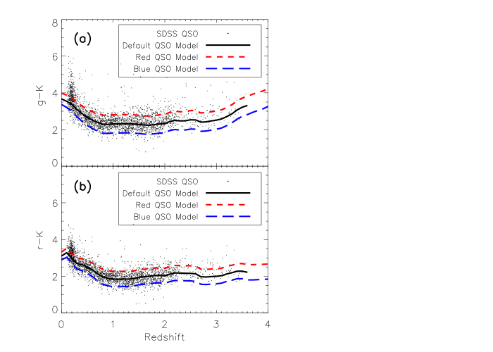
Figure 1: Colours of the bright SDSS DR3 quasar subsample, the median quasar model, a red quasar model, and a blue quasar model. (a) $g-K$; (b) $r-K$. The cluster of redder objects at very low redshift are mostly flagged as ‘extended’ in the DR3 quasar catalogue.

Comparison of the model quasar SED with the recently released optical–NIR empirical composite of Glikman, Helfand & White (2005) shows striking similarily, with a few differences. Most notably, the model quasar is somewhat redder at longer wavelengths, causing the derived K-corrections to be larger, particularly at $z<1$.

Composite, quasar plus host-galaxy SEDs are constructed via a simple sum of quasar and galaxy fluxes. The fraction of quasar and galaxy contributing to the combined SED is specified by the ratio of the respective fluxes over the restframe interval $4000-5000$ Å.

2.3 Host Galaxy SED/Evolution

Due to the very different shapes of quasar and galaxy SEDs, light from the host galaxy of a quasar will be most important at longer wavelengths, particularly around $\lambda$=12 000 Å. A series of studies (see Table 1) have found that, for bright quasars, the host galaxies are massive, bright ellipticals. The hosts of less luminous AGN have been found to have disc components (e.g. Dunlop et al. 2003; Kauffmann et al. 2003) with some evidence of recent star formation. The majority of quasars included in the simulations presented here are of at least moderate luminosity, and thus likely to be hosted by an early-type galaxy. However, we have investigated the effect of different galaxy SEDs by utilising the redshift zero template elliptical and Sb galaxies from Mannucci et al. (2001). The use of the two SEDs should encompass the range of galaxy types expected at the redshifts ($z\la 1$) where the presence of the galaxy is significant. The star formation histories of later-type galaxies can take a variety of forms and, for simplicity, the SEDs of both galaxy types do not evolve with redshift.

The adopted relationships between the quasar and host galaxy luminosity are described in Section 3.2. One of the relationships investigated is based on the brightness distribution of host galaxies at $z\sim 0.2$ (Section 3.1), which are then allowed to brighten with increasing redshift to take account of passive stellar evolution. The baseline evolution of the galaxy luminosity with redshift has been taken from a Bruzual & Charlot (2003, hereinafter BC2003) model of a stellar population formed at $z=5$ in a single burst with an exponential decay $\tau=1\,$Gyr. The passive evolution of an old stellar population is appropriate for the elliptical SED and we perform a specific test (Section 5.5) to confirm that the results of the simulations are not sensitive to significantly more rapid evolution in luminosity with redshift.

In some of the simulations, a fraction of the quasars are located in very luminous galaxies. To ensure that such galaxies do not evolve to become brighter than any known galaxy, a single upper limit to the luminosity achieved by any galaxy at a given redshift is adopted. The limit at $z=0$ is taken as $M(b_{J})=-22.4$ (i.e. 2 magnitudes brighter than the redshift zero value for $M^{*}$ of $-20.4$ from the 2dFGRS, Norberg et al. 2002), then adjusted at each redshift to take account of the BC2003 model luminosity evolution.

Table 1: Quasar and host galaxy properties of several studies investigated. Host galaxy properties resulting from the simulations were compared to these values where appropriate.

Ref.a	Redshift	Mqsob,c,d	Radio?	Selection	Mgal	$R_{1/2}$b	Morphology
		($b_{J}$)			($b_{J}$)	(kpc)
Schade	$0.03-0.15$	$-23.5<M<-13.9$	RQ	Xray	$-22.6<M<-17.8$	$0.2-18.1$	mostly E, few Sab
Dunlop	$0.10-0.25$	$-24.7<M<-20.4$	RQ,RL	Radio, Optical	$-22.5<M<-20.4$	$2.5-14.8$	mostly E
Floyd	$0.297-0.43$	$-26.7<M<-23.1$	RL,RQ	Optical	$-23.1<M<-20.8$	$1.3-15.3$	mostly E
Croom	$0.1-\sim 3$	$-28.68<M<-18.43$	–	Optical	$-27.9<M<-17.6$	–	assumed E SED

^a Schade, Boyle & Letawsky 2000; Dunlop et al. 2003; Floyd et al. 2004; Croom et al. 2002
^b Magnitudes and scalelengths have been converted to concordance cosmology
^c $B$-band AB magnitudes have been converted to Vega magnitudes using $B_{AB}-B=-0.1$
^d The following offsets have been used to convert from the passband the individual studies were performed in to $b_{J}$: $b_{J}-B=-0.055$, $b_{J}-V=0.09$, $b_{J}-R=0.52$ for quasars, and $b_{J}-B=-0.15$, $b_{J}-V=0.783$, $b_{J}-R=1.395$ for an elliptical galaxy. The conversions for an Sb galaxy are very similar to those for an elliptical galaxy.

3 The Distribution of Host Galaxy Magnitudes

Although it is clear that most bright quasars are hosted by elliptical galaxies, the observed brightnesses of the galaxies range significantly for a given quasar luminosity (see references contained within Table 1). It has been shown that the mass of the central black hole and the mass of its host galaxy bulge component are related via the Magorrian relation (Magorrian et al. 1998), which would suggest a linear correlation between quasar and galaxy magnitudes, but quasar fuelling efficiency and obscuring dust would tend to complicate the relation. Quasars of a given magnitude may therefore be found in galaxies of a variety of magnitudes, an observational result further reinforced by recent simulation work by Lidz et al. (2005), among others. The distribution of host galaxy magnitudes for a given quasar luminosity is as yet unknown. This has prompted us to devise a method for determining the distribution using the information contained within the SDSS DR3 quasar catalogue.

3.1 Host Galaxy Magnitudes from SDSS Quasars

In contrast to the 2QZ survey, which selects only blue point sources as candidates, the SDSS quasar selection algorithm does not discriminate with regard to the observed morphology of targets. Therefore, the bright subset of DR3 quasars (Section 2.2) may be divided into point source and extended objects, and two separate composite spectra created. The extended source composite spectrum shows strong stellar absorption lines, indicating the presence of host galaxy light entering into the spectroscopic fibre. The EWs of the absorption lines, when compared to the EWs from a redshift zero elliptical galaxy template from Mannucci et al. (2001), implies that the host galaxies contribute $\sim 50$ per cent of the total flux to the objects. Much weaker absorption lines, corresponding to a host galaxy contribution of 5–10 per cent, are found in the composite created from the objects classified as point sources. Given the large fraction of starlight evident in the quasar spectra, the question of the impact on the SDSS PSF magnitudes, recommended for use with point sources, arises.

The SDSS photometric catalogue provides both Petrosian and PSF magnitudes for sources. The Petrosian magnitudes (Petrosian 1976) measure a close to constant fraction of the total flux received from extended objects by defining a characteristic Petrosian radius and summing the flux within that radius. The PSF magnitude is measured by fitting a scaled PSF model to the object. This method provides an accurate measurement of the flux received from point-like objects such as stars or bright quasars. All magnitudes included in the SDSS quasar catalogues are PSF magnitudes, which will contain a certain amount of flux from the quasar host galaxies, particularly for low redshift, resolved objects (Schneider et al. 2003). The presence of the host galaxy will affect both the total flux and the colours of the objects.

Fig. 2 shows the distribution of PSF $g-r$ colour vs redshift for a low-redshift ($0.1<z<0.3$) sub-sample of the quasar sample, defined in Section 2.2, with magnitudes $15.6<g<18.8$ ($-24.8<M_{g}<-21.3$). The redshift range is narrow, so there should not be any significant evolution effect. The solid lines show the $g-r$ colour of an elliptical galaxy (top) and a quasar created as described in Section 2.2 (bottom), between $0.0<z<0.5$. The dashed lines, from bottom to top, show the $g-r$ colours for synthetic quasars that have increasing amounts of light from an elliptical galaxy contributing to the overall shape of the combined SED. The relative amount of galaxy and quasar flux is parametrized as follows, with $R_{gq}=0$ for a quasar and $R_{gq}=1$ for a galaxy:

$$R_{gq}=\frac{F_{galaxy}}{F_{galaxy+quasar}}$$

where $F_{galaxy}$ is the flux of the galaxy over the restframe interval $4000-5000\,$Å and $F_{galaxy+quasar}$ is the combined flux of the galaxy and quasar over the same wavelength interval. The synthetic colours correspond to Petrosian measures, as they include the total flux from both the quasar and host galaxy. Crosses mark the objects that were classified as point sources by the SDSS photometric pipeline (Lupton et al. 2001), while circles mark objects that were classified as extended. The stellar sources have colours that cluster around the $g-r$ colour calculated from the pure quasar SED, but the non-stellar objects show a much larger spread in colour, with some objects consistent with significant light from a host galaxy.

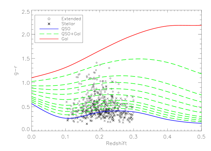
Figure 2: PSF $g-r$ colour of the bright subsample of SDSS DR3 quasars (crosses and circles). Also shown are the $g-r$ colours for an elliptical galaxy (top), the default quasar (bottom), and synthetic quasar+galaxy spectra for $0<R_{gq}<1$. The $R_{gq}$ values of the dashed lines, from bottom to top, are: 0.05, 0.1, 0.15, 0.2, 0.3, 0.4, 0.5, 0.6 and 0.8.

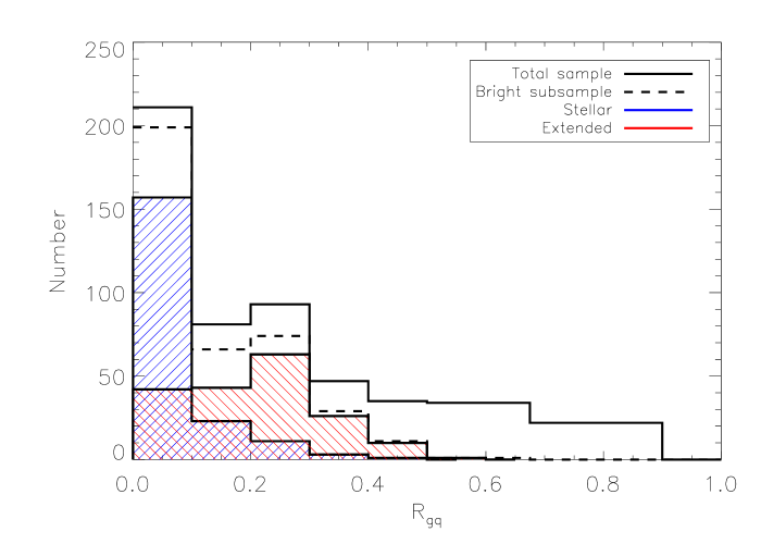
Figure 3: Histogram of $R_{gq}$ values derived from the Petrosian magnitude $g-r$ colours of the bright subsample of DR3 quasars. The $R_{gq}$ values have been binned.

When the same plot is created using the Petrosian magnitudes of the objects, the colours are skewed to larger $g-r$ values, indicating a larger contribution to the total flux from an extended component. The presence of i) spectral signatures due to starlight in the SDSS spectra, ii) a systematic trend between the $g-r$ colours and the morphological classification, iii) the strengthening of the trend when Petrosian magnitudes are employed, provides strong support for the presence of host galaxies as the dominant contribution to the extended distribution of $g-r$ colours. Furthermore, the distribution of $g-r$ colours is in excellent agreement with the model predictions for the colours of pure quasar and composite object SEDs which contain approximately equal contributions of quasar and elliptical galaxy light.

Fig. 2 is shown purely for illustration purposes. In order to correctly determine the fraction of galaxy flux contributing to each object, the Petrosian magnitudes must be used. Assuming the object SEDs are composed of a combination of quasar and galaxy light and that the Petrosian magnitudes provide an accurate measure of the total flux, then the position of an object on the $(g-r)$, redshift plane in relation to the model colours for composite SEDs gives a measure of the relative proportions of quasar and host galaxy light present in each object. The total object flux may then be separated into pure galaxy and pure quasar contributions, from which the magnitudes of each may be calculated.

As a result of the decomposition of the object magnitudes into their component brightnesses, 30 per cent of the sample possess quasar magnitudes that do not meet the absolute magnitude selection criterion of $M_{i}<-22.4$ used in the compilation of the SDSS DR3 quasar catalogue. Most of the excluded objects have large $g-r$ colours, but a significant number lie close to the faint magnitude limit and have $g-r$ colours consistent with only $\sim$ 30 per cent galaxy contribution (i.e. $R_{gq}=0.3$). It will be important for investigations of the form of the QLF at low redshifts using the SDSS sample to incorporate the effect of host galaxies on object magnitudes.

Excluding the objects that do not satisfy the absolute magnitude criterion leaves a quasar sample, in a narrow redshift range, for which the empirical distribution of $R_{gq}$ is now known. The distribution of $R_{gq}$, shown in Fig. 3, is used to determine the value and relative weighting of the constants describing the relation between quasars and their host galaxies in Section 3.2. We also have an empirical estimate, (Fig. 4) of the distribution of host galaxy magnitudes for quasars found in the SDSS survey at redshift $z\sim 0.2$.

Figure 4: Histogram of extracted host galaxy magnitudes from the bright, low redshift SDSS DR3 quasar sample, from the Petrosian magnitudes.

3.2 Quasar–Host Galaxy Luminosity Relationships

For the simulations, each quasar must be assigned to a host galaxy of a given brightness. Adopting a simple power law relationship, $L_{gal}\propto L_{qso}^{\gamma}$, or equivalently, expressed in magnitudes, $M_{gal}=A+\gamma M_{qso}$ with $A$ being a normalisation constant, there are essentially three possible parametrizations. First, at one extreme, the magnitudes of the quasar and its host galaxy are unrelated, corresponding to the case of $\gamma$=0.

But, since quasars of a given brightness are found in galaxies of a variety of brightnesses, a distribution of initial galaxy magnitudes, or constants $A$, is required. The empirical distribution found from Fig. 4 is used to determine the range and relative weighting of the constants, $A$. The SDSS $g$ passband is very similar to the $b_{J}$ passband and $b_{J}=g$ has been adopted without the use of a colour term. For this $\gamma$=0 case, the galaxies are then assumed to brighten due to passive stellar evolution according to the BC2003 prescription described in Section 2.3.

Alternatively, the quasar and galaxy magnitudes may be related with $0<\gamma\leq 1$. Croom et al. (2002) use the 2QZ+6QZ data set to find $\gamma$=0.42 and the constant $A=-11.10$. This normalisation is not expected to be representative because their sample excludes resolved objects, removing quasars with significant host galaxies. A range of normalisations for the Croom et al. relation was determined using the same quasar sample as above (Section 3.1). The resulting relative frequency of quasars with a host galaxy contributing a given fraction of the total brightness is shown in Fig. 3. The same procedure was adopted to determine the range and relative weightings of the constants $A$ for the third case, in which the brightnesses of quasars and their host galaxies follow the Magorrian relation, where $\gamma$ equals unity.

4 Simulation Program

All of the number-magnitude and number-redshift computations are performed in IDL, with the equations for cosmological quantities such as the distance modulus and comoving volume taken from Hogg (2000). Each simulation in a particular band is minimally parametrized by a QLF, bright and faint apparent magnitude limits, a range in redshift, and the K-correction values as a function of redshift. Additional options that may be specified include colour cuts to duplicate realistic surveys, magnitude errors and a prescription for the addition of host galaxy light to the quasars.

In real surveys there is generally some type of morphological selection applied, aimed at eliminating objects that are dominated by the host galaxy. To accommodate such selection, each simulation includes a restriction on the maximum fraction of the total light from the host galaxy, set at $R_{gq}<0.8$ (see Section 3.1 for definition). The $R_{gq}$ limit approximates the effect of morphological selection.

Every simulation also contains a faint absolute magnitude restriction on the total brightness of each object, as listed in Table 2. When host galaxy light is added, an additional faint magnitude limit of $M_{b_{J}}<-21$ is imposed on the quasar light alone thus ensuring intrinsically faint AGN are not boosted into the sample by the host galaxy light.

Measurement errors on the magnitudes of the objects are also included. The errors for $b_{J}$ are from Smith et al. (2005), and the SDSS DR3 catalogue (Schneider et al. 2005) for the SDSS $i$ and $K_{\rm 2MASS}$ passband errors. For the UKIDSS LAS, the errors are calculated using the magnitudes quoted on the UKIDSS website. Due to the relatively small errors for most of the simulations ($\lesssim$10 per cent), the effect on the final results is small.

The specified redshift range is divided into slices, and at each slice a luminosity function is created that covers the magnitudes accessible at that redshift, thus providing the number of objects at each magnitude at each redshift. If galaxy light is being added, the shape of the luminosity function will change due to the extra flux from the galaxies. The integral of the luminosity function at a specific redshift slice gives the number of objects at that redshift, or n(z). The sum over all redshifts within a small magnitude interval produces the number of objects at each apparent magnitude, or n(m).

5 Results

As described above, a QLF, a representative quasar SED, a galaxy SED and a relation between the magnitudes of the quasar and its host galaxy have been combined to produce number-redshift and differential number-magnitude counts for simulated surveys in the $b_{J}$, SDSS $i$, WFCAM $Y$ and $K$, and $K_{\rm 2MASS}$ passbands, over the redshift range $0.1<z<3.0$. Table 2 lists the parameters adopted for each survey. The faint absolute magnitude limits applied to every simulation are derived from the SDSS limit of $M_{i}<-22.4$, which is then converted to the other bands via the $z=0$ quasar colours.

The following subsections outline the results of the simulations, and highlight notable effects. As anticipated, host galaxy light has a significant effect on number-redshift relations, particularly for simulations in the near-infrared. The detailed shape of the galaxy SED has little effect, whereas the results are very sensitive to the shape of the quasar SED. Each prescription for adding host galaxy light increases number counts, but the redshifts and magnitudes of the objects most affected vary. Imposing a restriction on the fraction of host galaxy compared to the total flux, which approximates a morphological restriction, also becomes important, particularly at low redshifts.

Table 2: Simulated Surveys

Survey Name	Magnitude Range	Magnitude Limit	Morphological Restriction	Quasar Only	Quasar + Galaxy
			(input catalogue)	(N deg-2)	(N deg-2)
2QZ$+$6QZ	16.0 $<b_{J}<$ 20.85	M${}_{b_{J}}<-22.0$	Stellar	52.4	52.9
SDSS	16.0 $<i<$ 20.5	M${}_{i}<-22.4$	None	63.7	66.1
2MASS	12.0 $<K_{\rm 2MASS}<$ 15.0	M${}_{K_{\rm 2MASS}}<-25.6$	None	0.28	0.52
UKIDSS LASa	15.5 $<Y<$ 20.5	M${}_{Y}<-22.78$	None	81.7	88.1
UKIDSS LAS	14.0 $<K<$ 18.5	M${}_{K}<-25.7$	None	55.0	70.5

^a Large Area Survey

5.1 Initial Assessment

Fig. 5 shows the effect that adding host galaxy light to the flux of the quasars has on the shape of the QLF at $z=0.1$ and relatively faint magnitudes. The slope of the faint end is steepened significantly and the overall normalisation is increased. This effect decreases with increasing redshift, as the quasars become brighter and galaxy light is less significant.

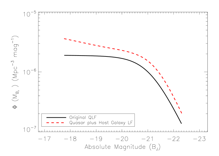
Figure 5: QLF before and after adding light from the host galaxy at $z=0.1$.

Figs. 6 and 7 are the number-redshift and differential number-magnitude relationships, respectively, that result from both the unaltered QLF and the LF when host galaxy light has been added, for a relatively shallow simulation corresponding approximately to 2MASS in the $K_{\rm 2MASS}$-band. The number-redshift counts are significantly increased at low redshifts, with the high redshift number counts remaining essentially the same. Fig. 7 shows that the number of objects detected at every magnitude is approximately doubled when host galaxy light is included. The number-redshift relationships for the other simulations listed in Table 2 are shown in Figs. 8(a) through (d), showing the increasing importance of host galaxy light at longer wavelengths. The concave shape of the n(z) curves at redshifts less than $\sim 1$ is due to the respective faint absolute magnitude restrictions on each simulation. This cut is particularly significant for the UKIDSS LAS $K$-band simulation, which has a relatively faint apparent magnitude limit, and thus many low redshift objects are eliminated. It is also worth noting in Fig. 8(d), that the presence of host galaxy light has a non-negligible effect on the number counts at redshifts as high as $z\sim$2.

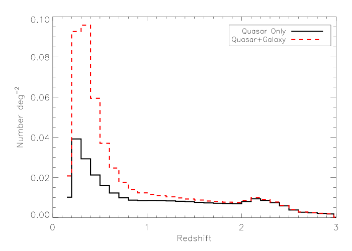
Figure 6: Number-redshift, n(z), relationship for $12<K_{\rm 2MASS}<15$, $0.1<z<3.0$ simulation.

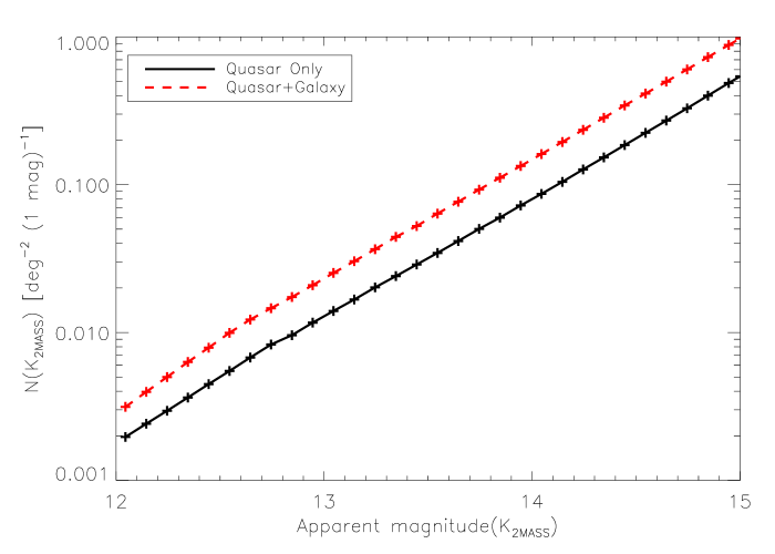
Figure 7: Differential number-magnitude, n(m), relationship for $12<K_{\rm 2MASS}<15$, $0.1<z<3.0$ simulation.

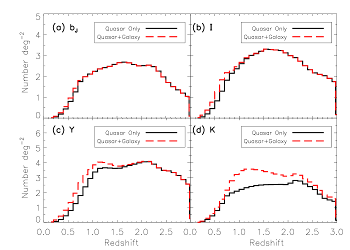
Figure 8: Number-redshift, n(z), relationships for simulations listed in Table 2. (a) 2QZ+6QZ $b_{J}$; (b) SDSS $i$; (c) UKIDSS LAS $Y$; (d) UKIDSS LAS $K$.

5.2 Quasar SEDs

The importance of the overall SED shape is illustrated in Figs. 9 and 10. As seen in Fig. 9(a), the K-correction derived from a pure power-law of spectral index $\alpha=-0.3$ is a good approximation to the K-correction from the default quasar SED in $b_{J}$ over the redshift range $0<z<3$, except for the lack of features due to emission lines within the passband. Fig. 9(b) shows that the bluer ($\alpha=0.0$) quasar SED increases the number counts at each redshift and the redder ($\alpha=-0.6$) SED decreases the number counts, as expected.

The situation is dramatically different for a near-infrared passband, as shown for $K_{\rm 2MASS}$ in Fig. 10. Comparing predictions for the default quasar SED against those for a quasar SED where the blue $\alpha=-0.3$ power law continuum extends all the way to $25\,000\,$Å, illustrates the effect of the inflection in the slope of the SED, at $\lambda\sim$12 000 Å, on the low redshift number counts. At $z>1$, the n(z)’s derived from the default and power-law SEDs (Fig. 10(b), solid and dotted histograms) come more into line, as the identical restframe optical portion of the SEDs become increasingly important.

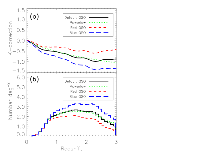
Figure 9: Effect of quasar SED shape on number-redshift counts, for the 2QZ+6QZ simulation in $b_{J}$. (a) The default QSO SED, a pure power-law with $\alpha=-0.3$, red QSO SED with $\alpha=-0.6$, blue QSO SED with $\alpha=0.0$; (b) number-redshift counts for each of the SEDs.

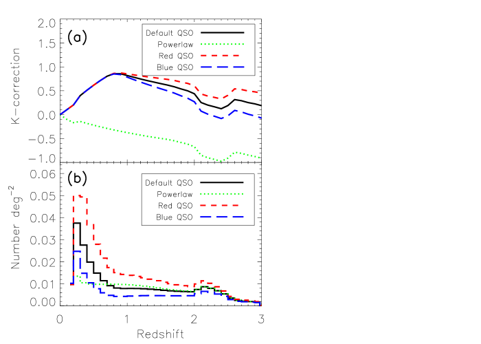
Figure 10: Effect of quasar SED shape on number-redshift counts, for the 2MASS simulation in $K_{\rm 2MASS}$. (a) The default QSO SED, a power-law with $\alpha=-0.3$ and emission lines, red QSO SED with $\alpha=-0.6$, blue QSO SED with $\alpha=0.0$; (b) number-redshift counts for each of the SEDs.

5.3 Galaxy SEDs

Although it has been shown that using an appropriate quasar SED can have significant effects on the number-redshift and number-magnitude relations derived from the simulations, the exact form of the galaxy SED incorporated has much less of an effect. Figs. 11(a) and (b) show the relatively small impact in the $K$-band, for both a deep and a shallow survey, due to the differences between the elliptical and Sb host galaxy SEDs. The presence of host galaxy light is much more important than the detailed shape of the SED. The two curves converge at $z\approx 2$ due to the restframe wavelength interval at which the quasar and host galaxy SEDs are normalised moving into the $K$-band (see Section 2.2).

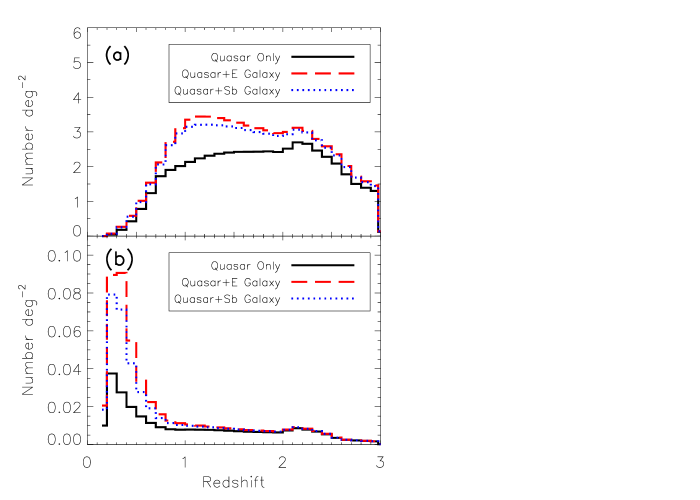
Figure 11: Difference between adding an early type galaxy and an Sb galaxy to quasar flux. (a) Simulation corresponding to UKIDSS LAS in $K$; (b) Simulation corresponding to 2MASS in $K_{\rm 2MASS}$. Note the different y scales.

5.4 Quasar–Galaxy Relationships

While the predictions are not very sensitive to the details of the host galaxy SED, the prescription determining the brightness of the host galaxy relative to the quasar has a major impact on the near-infrared number counts (Fig. 12).

Setting $\gamma$=0, every quasar at a given redshift is assigned to the same galaxy. This has very little effect when the galaxy is faint, but when a relatively bright galaxy is added, the faint quasars are now dominated by the host galaxy light. At higher redshifts, when all of the objects are much brighter than the set galaxy magnitudes, almost no effect is detectable, as seen in Fig. 12(b).

The $\gamma$=1 case is very different. Each quasar at a given redshift brightens in magnitude by the same amount when the galaxy flux is added, effectively shifting the QLF brightward. Because neither faint nor bright objects are preferentially affected in this scheme, the number counts are increased almost equally at all redshifts, as seen in Fig. 12(a).

Unsurprisingly, the $\gamma$=0.42 case produces intermediate behaviour. Relatively faint quasars are assigned to relatively faint host galaxies, while the brighter quasars end up in brighter galaxies, with a smooth transition in between. The counts are increased at low redshift, to a somewhat lesser degree than for $\gamma$=0, with a decreasing effect as redshift increases and the quasars become much brighter than their hosts.

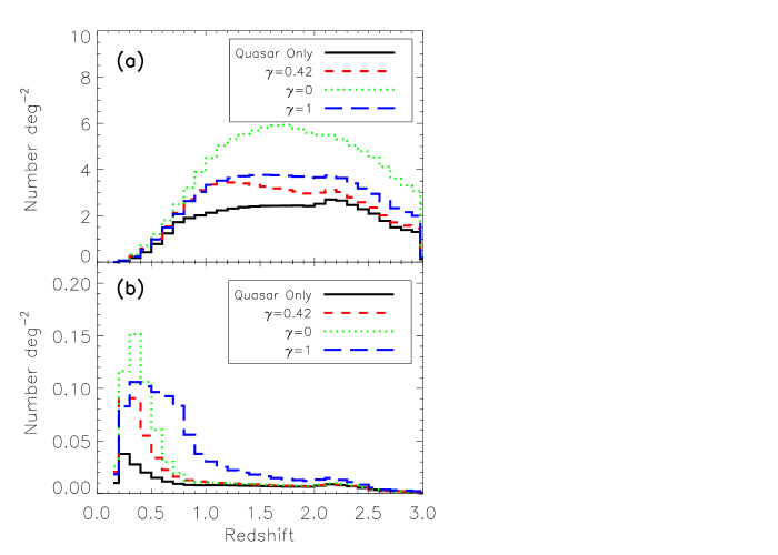
Figure 12: Comparison of prescriptions for adding galaxy light. (a) Simulation corresponding to UKIDSS LAS in $K$; (b) Simulation corresponding to 2MASS in $K_{\rm 2MASS}$. Note the different y scales.

5.5 Galaxy Luminosity Evolution

In the case of the empirical correlations between host galaxy and quasar luminosity, with $\gamma$=0.42 and $\gamma$=1, the BC2003 passive evolution model adopted for the change in galaxy luminosity only affects the maximum brightness a galaxy may obtain, at a given redshift. None of the simulations are sensitive to sensible changes in the adopted values for the maximum achievable galaxy luminosity.

In the case of the $\gamma$=0 model, with the galaxy luminosities evolving according to the adopted BC2003 passive evolution predictions, changes to the rate of evolution can have a significant effect. As an illustration, the galaxies were allowed to become 0.5 mag brighter than the passive evolution case, modelled as a linear increase in brightness as a function of lookback time over the range $0.0<z<4.0$. There is little discernable effect at low redshifts, as the luminosity increase is small, but for a near-infrared survey that probes to faint quasar luminosities at significant redshifts, the increase in numbers can be large. The origin of the increase is the fraction of intrinsically faint quasars in luminous host galaxies, where the increase in the host galaxy luminosity evolution brings additional quasars above the faint magnitude limit (Fig. 13). Such objects are, essentially by definition, dominated by galaxy light and the inclusion of a morphological restriction, such that $R_{gq}<0.8$, effectively removes the additional population. The significant changes in the fraction of host galaxy-dominated systems at high redshift in surveys to faint flux limits in the near-infrared illustrates the potential importance of the host galaxy on the number of quasars appearing above the survey flux limit.

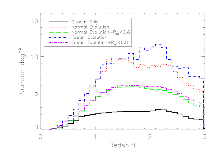
Figure 13: Comparison of galaxy brightness evolution, with and without a morphological restriction $R_{gq}<0.8$ imposed. Simulation corresponding to UKIDSS LAS in $K$.

5.6 Morphological Selection Criteria

It is clear from previous sections that the initial morphological selection criteria applied to define a candidate quasar sample can be important in certain circumstances. The conservative limit of $R_{gq}<0.8$ adopted above is chosen to approximate the fraction of host galaxy light that would result in an object being classified as a galaxy rather than a quasar, and thus excluded from a quasar sample. From Fig. 2, it can be seen that for $R_{gq}>0.3$ almost all objects are classified as extended in the SDSS catalogue. Therefore, $R_{gq}=0.3$ may be taken as the approximate fraction of galaxy light that is required for an object to appear non-stellar when relatively high-quality imaging observations are available.

Figs. 14(a) and (b) show the results from applying the more stringent morphological restriction for the UKIDSS and 2MASS $K$-band surveys, respectively, using the $\gamma$=0.42 host galaxy prescription. The main difference appears at low redshifts, where the quasars are of moderate luminosity and the host galaxies contribute significantly to the total light. As anticipated, there is little difference at high redshifts, where the objects are dominated by the quasar light.

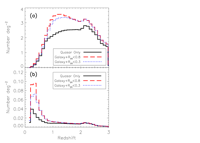
Figure 14: Number-redshift relations for morphological selection criteria set at $R_{gq}<0.8$ and $R_{gq}<0.3$. (a) Simulation corresponding to UKIDSS LAS in $K$; (b) Simulation corresponding to 2MASS in $K_{\rm 2MASS}$. Note the different y scales.

6 Discussion

6.1 Initial Assessment

Confidence in the results is gained by comparing the calculated number-magnitude and number-redshift relations with results from existing surveys. The excellent agreement between the predictions incorporating the distribution of host galaxy luminosities from the SDSS $i$-band sample, for 2QZ+6QZ in the $b_{J}$-band confirm that the presence of host galaxies has not biased significantly the determinations of the QLF from observations at blue wavelengths.

There is also good agreement between the predicted number counts in the $i$-band and the published SDSS results to $i\sim 19.0$, which indicates that the fraction of reddened quasars missing from a $b_{J}$-selected sample but visible in the $i$-band, at nearly twice the observed-frame wavelength, is not large.

As seen in Figs. 5 through 8, employing an SED that represents the median quasar over a large range of wavelengths and adding a prescribed amount of host galaxy light mostly affect the low redshift ($z\lesssim 1$) number counts, particularly at longer wavelengths. Hardly any effect is seen at $z\gtrsim 1.5$ except for the UKIDSS LAS $K$-band simulation, where the faint magnitude limits enable intrinsically faint quasars to be detected to high redshifts. In fact, the UKIDSS LAS survey probes approximately one magnitude fainter down the QLF than does the 2QZ survey.

Morphological and colour restrictions applied to define quasar candidate samples need to be considered in order to avoid contamination from the many low-redshift galaxy-dominated objects while allowing the resolved quasars to be included. The results are relevant to the design of future surveys as depths and areas required to observe a given number of unobscured objects are now known. For example, the area of sky in the UKIDSS LAS needed to establish the existence of a given fraction of obscured quasars may be readily calculated.

6.2 Quasar SEDs

The adoption of a single power-law approximation to the form of the restframe quasar continuum over $1200<\lambda<5000\,$Å has proved largely adequate for surveys in the optical out to redshifts $z\sim 2.5$. Extending observations into the near-infrared highlights the inadequacy of the single power-law approximation. Incorporation of the strong inflection in the SED at $\lambda\sim$12 000 Å is essential in order to understand observations at near-infrared wavelengths. Fig. 10(a) illustrates the dramatic difference in the K-correction at $z\lesssim 1$. The effect on the optical–NIR colours of the quasars is large and the observed behaviour is sometimes misattributed to the presence of the host galaxy making the colours much redder, as in figure 7 of Glikman et al. (2004). Fig. 1 shows both the reddening of the optical–NIR colour from the SED at $z\lesssim 1$ as well as the effect of the host galaxy, seen only at $z\lesssim 0.3$. The shape of the SED and the presence of host galaxy clearly produce different signatures. Fig. 10(b) shows the combined impact on the number of objects observed at $z\lesssim 1$ at bright near-infrared magnitudes.

The simulation predictions are very conservative in the sense that an object contributing to the counts must have a minimum quasar absolute magnitude of $M_{b_{J}}=-21.0$, equivalent to $M_{K_{\rm 2MASS}}=-24.6$. The objects identified as AGN in 2MASS by Cutri et al. (2002) and Francis et al. (2004) have no such limit applied. Furthermore, while a $J-K>2.0$ is often taken as a definition of a ‘red’ AGN, our default quasar SED has $J_{\rm 2MASS}-K_{\rm 2MASS}=2.5$ at $z=0.0$ and a non-negligible fraction of optically-selected quasars possess $J-K\geq 2.0$ at low redshift. The impact of adopting fainter absolute magnitude limits for ‘quasar’ samples, plus the effect of any additional colour selection criteria applied, need to be carefully assessed before reliable conclusions concerning any excess of objects over that predicted on the basis of optical samples can be reached.

6.3 Quasar–Galaxy Relationships

Given our lack of knowledge concerning the distribution of host galaxy luminosities as a function of quasar luminosity the relations adopted in the simulations deliberately span an extended range in possible behaviour. One extreme, ($\gamma$=1), is motivated by theoretical arguments from known relations between the mass of black holes and the mass of their host bulges. The distribution of $R_{gq}$ then approximates the range of accretion rates and efficiencies present in the population.

The other extreme, ($\gamma$=0), where there is no relationship between quasar and host galaxy luminosity, approximates a situation in which any underlying relation between quasar and galaxy properties is overwhelmed by variations in accretion rates and efficiency (relative to the Eddington luminosity).

Intermediate between the two extremes, the $\gamma$=0.42 case is observationally motivated (Croom et al. 2002). Such an observed relationship is perhaps not unexpected on theoretical grounds but the general applicability of the Croom et al. (2002) relationship remains to be established. The quasars included in their study cover a relatively modest range in redshift/luminosity and there must still be concerns over the exclusion of objects with substantial galaxy contributions. The fractional galaxy contribution was estimated from fibre spectra and Croom et al.’s claim that the fraction of host galaxy light that enters the fibre is effectively constant with redshift relies on assumptions concerning the host galaxy sizes and should be investigated quantitatively. However, we have chosen to adopt the $\gamma$=0.42 case as the default for the simulations.

The key result of the simulations, in Section 5.4, is the significant impact of the presence of host galaxy light on the surveys in the near-infrared. The n(z) results for both of the $K$-band simulations are shown in Fig. 12. The three prescriptions for adding host galaxy light affect different portions of the QLF at a given redshift. When $\gamma$=1, the galaxies increase in brightness at the same rate as the quasars in this case, thus the n(z) relation is affected to higher redshifts. As can be seen in Fig. 12(a) the n(z) at $z\sim 2$ differ significantly among the host galaxy prescriptions, offering the prospect of constraining the relation between quasar and host galaxy luminosity at high redshifts.

The $\gamma$=0 prescription is unique in that some relatively low-luminosity quasars have bright host galaxies. The faint quasars are then dominated by the host galaxy light, producing a dramatic steepening of the observed QLF at faint luminosities. The effect is most evident at low redshifts, $z<1$, as the fractional contribution of host galaxy light decreases with increasing redshift, as the luminosity of the quasars increases faster than the passively evolving host galaxies. Whether such host galaxy-dominated objects feature prominently in a near-infrared survey depends on the morphological restriction imposed, since many very faint quasars are boosted above the faint magnitude limit of the simulation due almost entirely to light from the host galaxy. Requiring $R_{gq}<0.8$ ensures that host galaxy-dominated objects are excluded. Interpreting the results of surveys where host galaxy dominated objects are detected depends on the ability to estimate accurately the luminosity of the central source alone, so that relatively weak AGNs located in bright galaxies are not classified as quasars (c.f. Section 3.1). As an illustration of the importance of accurately separating quasar from host galaxy light, the study of White et al. (2003) found several red objects in an $i$-band selected sample. However, two of the four objects with the largest derived $E(B-V)$ values from their table 1, (J1011+5205, J1021+5114), were classified as non-stellar by the SDSS photometry. As both objects are at $z\sim 1$, they must be dominated by their host galaxies in order to be resolved, and the red colours of the objects almost certainly result in part from host galaxy light.

6.4 Selection Criteria and Survey Design

Morphological and colour selection applied to an object catalogue usually form an integral part of the identification of quasar candidates. A morphological restriction on object selection is approximated in the simulations by monitoring the fraction of host galaxy flux that is contributing to the total flux of each object, denoted $R_{gq}$. This restriction is only an approximation, as in practice the $R_{gq}$ value separating morphological classifications will be dependent on both the redshifts of the targets and the seeing conditions of the observations.

In the case of the 2QZ+6QZ survey, based on (by modern standards) relatively poor quality photographic imaging, the adoption of strict morphological selection turns out to have little impact on the fraction of the quasar population included. Changing the morphological restriction from $R_{gq}<0.8$ to $R_{gq}<0.3$ has almost no effect on the counts. The insensitivity to the presence of host galaxies arises due to a combination of the increasingly large contrast between quasar and galaxy flux at ultraviolet wavelengths and the relatively high lower redshift limit of $z_{low}=0.4$ imposed by Croom et al. (2002).

The same is not true for surveys in the near-infrared, as seen in Fig. 14. Excluding extended sources will certainly eliminate many low redshift quasars. The effect can also be seen by using the 2MASS magnitudes for the objects in the SDSS DR3 quasar catalogue. If the restriction of requiring point-like morphology is imposed on the DR3 quasars, n(m) and n(z) counts in $K_{\rm 2MASS}$ agree well with the quasar-only $K_{\rm 2MASS}$ simulation, further reinforcing the importance of adopting a realistic quasar SED parametrization. Relaxing the point-like restriction, to include resolved objects, results in n(m) and n(z) counts in $K_{\rm 2MASS}$ that agree well with the $K_{\rm 2MASS}$ simulation that includes host galaxy light limited at $R_{gq}<0.8$. The study by Francis et al. (2004), searching for dust-reddened quasars, selected objects from the 2MASS catalogue and found a higher surface density of $1\pm{0.3}$ quasar deg^-2 to $K_{\rm 2MASS}=15.0$. They note that some of their ‘quasars’ have optical colours indistinguishable from galaxies, and the objects are dominated by their host galaxies. They impose no morphological restriction on their sample, and some of their objects could easily have $R_{gq}$ values approaching unity and would thus be removed from our simulations.

It is clear from the discussion above that the inclusion of certain non-stellar objects in quasar candidate samples selected in the near-infrared will be necessary for many investigations. Of particular interest is the impact of the presence of host galaxy light on the colours of quasars and, thereby, on the effectiveness of colour-based selection schemes designed to isolate particular elements of the quasar population. For example, a key goal, now that faint $K$-band data from UKIDSS LAS and other surveys are becoming available, is to establish the fraction of reddened luminous quasars.

Warren, Hewett & Foltz (2000) introduced the KX-method of selection (by analogy with the UV-excess selection, or UVX) specifically to address the problem of isolating reddened quasars using a combination of optical and near-infrared colours. However, they did not consider the impact of host galaxy light on the proposed selection scheme. Fig. 15 shows the colour-colour diagram advocated by Warren et al. (2000). Shown are the default quasar and elliptical galaxy loci for redshifts $0.1<z<3.0$ and $0.1<z<2.0$, respectively, the locus of galactic dwarf stars, as well as quasar tracks with $0<R_{gq}<1$ at several redshifts. The crucial aspect of the KX-method is that reddened quasars move further away from the locus of galactic stars, which will be present in enormous numbers relative to the much rarer quasars. It can be seen immediately that the presence of the host galaxies moves the quasars redward in $r-J$. Of more potential concern is the horizontal displacement in $J-K$. At a fixed redshift, the locus of objects with $0<R_{gq}<1$ is indicated by the dotted line, joining the track (blue line) for the pure quasar, $R_{gq}=0$, to the track (red) for the pure galaxy, $R_{gq}=1$.

At low redshifts, $z\lesssim 0.3$, increasing the amount of host galaxy light makes the objects more blue in $J-K$, so very low redshift, $z<0.1$, galaxy-dominated objects will be excluded with a moderate colour cut, like the $J-K>1.2$ selection employed by Francis et al. (2004). Fortunately, the effect of the host galaxy light diminishes rapidly with increasing redshift and only for redshifts $z<0.1$ is proximity to the stellar locus an issue for the quasar selection. At $z\gtrsim 0.3$, increasing host galaxy contribution causes the objects to appear redder in $J-K$, improving the effectiveness of the KX-selection scheme. Note however that the sense of the colour changes for quasars with $0.5\lesssim z\lesssim 2$ are very similar to those due to simply reddening a pure quasar SED, highlighting the importance of quantifying the fraction of host galaxy light present when interpreting surveys for reddened quasars.

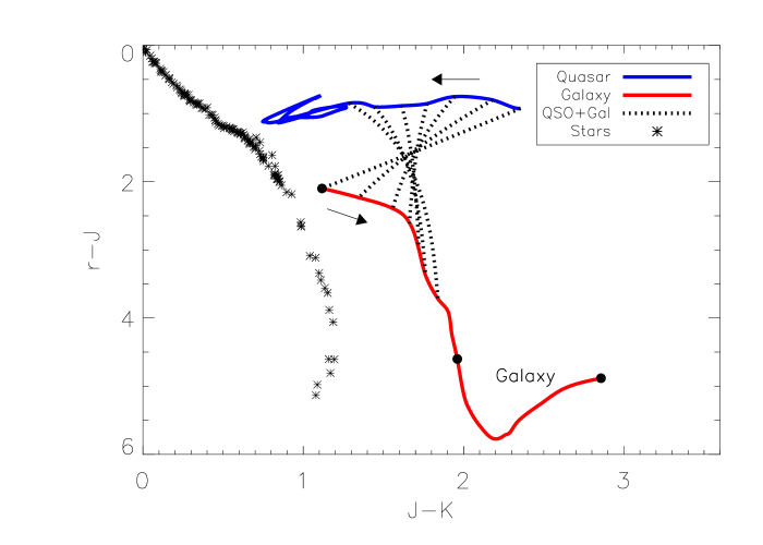
Figure 15: Colour-colour diagram showing the evolution of the quasar locus (top) for $0.1<z<3.0$ and galaxy locus (bottom) for $0.1<z<2.0$, as well as the location of the stellar locus for dwarf stars from the Bruzual-Persson-Gunn-Stryker Atlas included in the STSDAS SYNPHOT package. The dotted lines are for objects with $R_{gq}$ increasing from zero to unity, for redshifts 0.1, 0.2, 0.3, 0.4, 0.5, 0.6, and 0.7. Arrows indicate the direction of increasing redshift for the quasar and galaxy tracks, with the filled circles on the galaxy track marking redshifts 0.1, 1.0 and 2.0.

7 Summary

Simulations of quasar surveys ranging from optical to near-infrared wavelengths have been performed by combining current information on the quasar luminosity function and the quasar SED. Host galaxy light was added according to different prescriptions and has the most effect at longer wavelengths. The main results of this study are:

• The overall shape of the quasar SED is important, particularly the correct treatment of the continuum longward of 12 000 Å  for the surveys at near-infrared wavelengths.

• The near-infrared simulations produced many more galaxy-dominated objects than simulations at optical wavelengths and were much more affected by morphological restrictions, which should thus be chosen carefully if performing surveys at longer wavelengths.

• The simulations are not sensitive to the SED of the galaxy added to the quasar, but are sensitive to the prescription relating host galaxy and quasar luminosity.

The predictions presented should provide a reference for the contribution of the unobscured quasar population in near-infrared surveys, and are of direct relevance to the design of future surveys.

Appendix A The b_J passband

The $b_{J}$ passband was key in the compilation of the second period of all-sky photographic surveys that began in the 1970s with the programmes using the 1.2m United Kingdom Schmidt Telescope at Siding Spring in Australia (Cannon 1984) and continued with the initiation of the Palomar Observatory Sky Survey II (Reid et al. 1991) using the 1.2m Oschin Schmidt at Palomar Mountain in the United States of America. The resulting all-sky surveys have formed a critical part of modern astrophysical research, particularly in the form of the products from the digital scanning of the photographic plates (Lasker 1995).

Conventional colour equations relating $b_{J}$ to Johnson $B$ and $V$ were established at an early stage (Blair & Gilmore 1982). However, to our knowledge, no published determination of the response function for the $b_{J}$ passband exists in the astronomical literature. One of us (Hewett) made such a determination more than a decade ago and the resulting response function has been used in many investigations, frequently with a reference to ‘Hewett (private communication)’.

The basis for the determination of the $b_{J}$ passband is the unfiltered objective-prism plate UJ10738P, obtained on 1986 February 11, at a mean airmass of 1.3, with the United Kingdom Schmidt Telescope. The 55 minute exposure, on sensitised Kodak IIIaJ emulsion, of a portion of the Virgo Cluster was scanned by the APM Facility as part of the Large Bright Quasar Survey (Hewett, Foltz & Chaffee 1995). The follow-up observations of candidate quasars undertaken at the Multiple Mirror Telescope resulted in a large number of fluxed spectra of quasars and stars covering the wavelength range from the atmospheric cutoff at $\sim 3200\,$Å to $\sim 7500\,$Å, well beyond the red cutoff of the Kodak IIIaJ emulsion. It was therefore possible to make a direct empirical determination of the IIIaJ emulsion sensitivity by comparing the fluxed object spectra with the individual intensity scans of the corresponding objective-prism spectra from the APM.

The passband presented here is based on the use of $\sim 120$ spectra, each with corresponding unsaturated objective-prism spectra from the APM scans. The fluxed spectra were multiplied by an approximation to the wavelength dependent passband transmission (taken to be constant initially). A cutoff to the emulsion response, linear in wavelength, at the red end of the spectra was incorporated. The spectra were then rebinned to match the non-linear wavelength scale appropriate to the objective-prism spectra and convolved with a Moffat profile (Moffat 1969), to take account of the seeing. The resulting spectra were then compared to the corresponding objective-prism spectra. The fluxed and objective-prism spectra were normalised using the wavelength interval $4000-5000\,$Å. An approximation to the transmission at each wavelength was made by taking the median value at each wavelength of the 120 factors obtained by dividing each object-prism spectrum by the synthetic spectrum.

A $\chi^{2}$ measure of the goodness-of-fit for the new approximation to the transmission as a function of wavelength could then be obtained by including the new estimate at the initial stage of the process and calculating a $\chi^{2}$ value, over the full wavelength range for which the transmission is non-zero, using the resulting synthetic and actual objective-prism spectra. The procedure was incorporated into the AMOEBA routine from Numerical Recipes (Press et al. 1992) to determine the best-fit parameters describing the wavelength cutoff and the seeing, along with the wavelength dependent transmission. Technically, the wavelength dependent transmission should be determined independently by the routine, prior to blurring by the seeing. However, in practice, away from the relatively sharp emulsion cutoff, the effect of the seeing on the slowly varying transmission function is simply to apply a modest degree of smoothing. The synthetic spectra produced employing the final transmission function provide a superb match to the individual objective-prism spectra.

The resulting transmission function (Figure 16) represents the combination of atmosphere, telescope optics and the photographic emulsion. Transforming to a function appropriate to unit-, or zero-, airmass was achieved by correcting for extinction using the mean extinction curve for Kitt Peak, which is expected to be a good approximation for the Siding Spring site.

The objective-prism plate was obtained without any short-wavelength filter, with the decreasing transmission towards the blue due mainly to the effect of atmospheric extinction. The appropriate blue cutoff for the $b_{J}$ passband was applied using the transmission curve for a 2mm thick Schott GG395 filter. Note that the similar ‘$b_{J}$’ passband employed at several 4m-class telescopes in the 1980s employed a GG385 filter (e.g. Kron 1980).

The resulting transmission function is appropriate for calculating the magnitudes of objects recorded using detectors, such as photographic plates, that integrate energy per unit wavelength across the passband. The majority of modern detectors, such as CCDs, integrate photon counts across the passband and many synthetic photometry packages, such as STSDAS SYNPHOT, assume by default that the detector is a photon-counting device (see Bessell, Castelli & Plez (1998) for a more detailed discussion). In order to obtain the correct results for the $b_{J}$ passband using such packages it is necessary to modify the input transmission function, scaling the transmission by a factor of $1/\lambda$. Table 3 contains tabulations of the normalised $b_{J}$ passband transmissions suitable for use with energy- and photon-integration software packages.

Table 3: Relative Transmission for the $b_{J}$ Passband

Wavelength	Relative Transmission	Relative Transmissiona
(Å)
3540	0.000	0.000
3590	0.004	0.006
3640	0.022	0.031
3690	0.076	0.105
3740	0.150	0.207
3790	0.285	0.386
3840	0.420	0.562
3890	0.521	0.688
3940	0.604	0.788
3990	0.693	0.893
4040	0.724	0.920
4090	0.726	0.912
4140	0.721	0.896
4190	0.727	0.891
4240	0.720	0.873
4290	0.693	0.830
4340	0.679	0.804
4390	0.683	0.800
4440	0.686	0.794
4490	0.652	0.746
4540	0.672	0.761
4590	0.673	0.754
4640	0.738	0.817
4690	0.753	0.825
4740	0.762	0.826
4790	0.762	0.817
4840	0.763	0.810
4890	0.756	0.794
4940	0.783	0.815
4990	0.801	0.825
5040	0.855	0.872
5090	0.939	0.949
5140	1.000	1.000
5190	0.992	0.982
5240	0.851	0.834
5290	0.667	0.648
5340	0.494	0.476
5390	0.321	0.306
5440	0.134	0.127
5490	0.011	0.010
5540	0.000	0.000

^a Transmission values for use with software that assumes a photon counting detector

Figure 16: $b_{J}$ relative transmission function for energy integration detectors.

Appendix B Differential Number-Magnitude Tables

Tables containing the differential number-magnitude counts for each of the surveys simulated are given in Tables 4 through 8. The magnitude and redshift limits of the simulations are given in the caption of each table, and may also be found in Section 5. The definition of $R_{gq}$ is described in Section 3.1, and the prescription for adding host galaxy light to that of the quasar is taken from Croom et al. (2002), with $\gamma$=0.42. In each table, the first column gives the magnitude range for each entry, and the second column lists the number of objects predicted by simulations including only the quasar SED between the listed magnitudes. The third and fourth columns list the number of objects predicted by simulations that include host galaxy light, with limits of 80 and 30 per cent, respectively, imposed on the final galaxy light contributions.

Table 4: Differential number per 0.25 magnitude, deg^-2 for the survey in $b_{J}$, with magnitude limits of $16.0<b_{J}<20.85$ and a faint absolute magnitude limit for the total combined flux from quasar and host galaxy of $M_{b_{J}}<-22.0$, and redshifts $0.1<z<3.0$.

Magnitude	Quasar Only	Q+G	Q+G
		$R_{gq}<0.8$	$R_{gq}<0.3$
16.00 - 16.24	0.010	0.010	0.010
16.25 - 16.49	0.016	0.017	0.017
16.50 - 16.74	0.027	0.027	0.027
16.75 - 16.99	0.045	0.046	0.045
17.00 - 17.24	0.073	0.074	0.074
17.25 - 17.49	0.121	0.123	0.122
17.50 - 17.74	0.195	0.198	0.196
17.75 - 17.99	0.315	0.319	0.317
18.00 - 18.24	0.514	0.519	0.515
18.25 - 18.49	0.812	0.819	0.813
18.50 - 18.74	1.233	1.243	1.235
18.75 - 18.99	1.887	1.900	1.887
19.00 - 19.24	2.730	2.749	2.731
19.25 - 19.49	3.760	3.787	3.761
19.50 - 19.74	4.986	5.023	4.987
19.75 - 19.99	6.254	6.305	6.257
20.00 - 20.24	7.514	7.581	7.517
20.25 - 20.49	8.418	8.512	8.430
20.50 - 20.74	9.199	9.318	9.214
20.75 - 20.85	4.291	4.354	4.300
Total	52.40	52.93	52.46

Table 5: Differential number per 0.25 magnitude, deg^-2 for the survey in $i$, with magnitude limits of $16.0<i<20.5$ and a faint absolute magnitude limit for the total combined flux from quasar and host galaxy of $M_{i}<-22.4$, and redshifts $0.1<z<3.0$.

Magnitude	Quasar Only	Q+G	Q+G
		$R_{gq}<0.8$	$R_{gq}<0.3$
16.00 - 16.24	0.033	0.039	0.037
16.25 - 16.49	0.053	0.063	0.060
16.50 - 16.74	0.087	0.101	0.097
16.75 - 16.99	0.143	0.164	0.158
17.00 - 17.24	0.234	0.264	0.256
17.25 - 17.49	0.380	0.425	0.413
17.50 - 17.74	0.612	0.675	0.659
17.75 - 17.99	0.971	1.057	1.033
18.00 - 18.24	1.502	1.614	1.580
18.25 - 18.49	2.250	2.385	2.338
18.50 - 18.74	3.218	3.375	3.316
18.75 - 18.99	4.380	4.557	4.482
19.00 - 19.24	5.640	5.837	5.744
19.25 - 19.49	6.888	7.109	6.999
19.50 - 19.74	8.032	8.270	8.140
19.75 - 19.99	8.984	9.234	9.079
20.00 - 20.24	9.720	9.981	9.795
20.25 - 20.50	10.591	10.908	10.669
Total	63.720	66.058	64.852

Table 6: Differential number per 0.25 magnitude, deg^-2 for the survey in $K_{\rm 2MASS}$, with magnitude limits of $12.0<K_{\rm 2MASS}<15.0$ and a faint absolute magnitude limit for the total combined flux from quasar and host galaxy of $M_{K_{\rm 2MASS}}<-25.6$, and redshifts $0.1<z<3.0$.

Magnitude	Quasar Only	Q+G	Q+G
		$R_{gq}<0.8$	$R_{gq}<0.3$
12.00 - 12.24	0.001	0.001	0.001
12.25 - 12.49	0.001	0.002	0.001
12.50 - 12.74	0.002	0.003	0.002
12.75 - 12.99	0.003	0.005	0.004
13.00 - 13.24	0.004	0.007	0.006
13.25 - 13.49	0.006	0.012	0.010
13.50 - 13.74	0.010	0.018	0.016
13.75 - 13.99	0.016	0.029	0.025
14.00 - 14.24	0.025	0.047	0.040
14.25 - 14.49	0.040	0.075	0.065
14.50 - 14.74	0.065	0.120	0.106
14.75 - 15.00	0.111	0.203	0.182
Total	0.284	0.521	0.458

Table 7: Differential number per 0.25 magnitude, deg^-2 for the survey in $Y$, with magnitude limits of $15.5<Y<20.5$ and a faint absolute magnitude limit for the total combined flux from quasar and host galaxy of $M_{Y}<-22.78$, and redshifts $0.1<z<3.0$.

Magnitude	Quasar Only	Q+G	Q+G
		$R_{gq}<0.8$	$R_{gq}<0.3$
15.50 - 15.74	0.024	0.033	0.030
15.75 - 15.99	0.040	0.054	0.050
16.00 - 16.24	0.067	0.088	0.083
16.25 - 16.49	0.111	0.145	0.136
16.50 - 16.74	0.182	0.236	0.224
16.75 - 16.99	0.298	0.380	0.363
17.00 - 17.24	0.483	0.605	0.579
17.25 - 17.49	0.770	0.945	0.908
17.50 - 17.74	1.204	1.440	1.389
17.75 - 17.99	1.834	2.138	2.071
18.00 - 18.24	2.695	3.062	2.977
18.25 - 18.49	3.793	4.212	4.105
18.50 - 18.74	5.045	5.526	5.399
18.75 - 18.99	6.268	6.882	6.734
19.00 - 19.24	7.544	8.128	7.956
19.25 - 19.49	8.710	9.246	9.041
19.50 - 19.74	9.690	10.207	9.946
19.75 - 19.99	10.503	11.020	10.687
20.00 - 20.24	11.010	11.608	11.219
20.25 - 20.50	11.388	12.123	11.658
Total	81.658	88.076	85.555

Table 8: Differential number per 0.25 magnitude, deg^-2 for the survey in $K$, with magnitude limits of $14.0<K<18.5$ and a faint absolute magnitude limit for the total combined flux from quasar and host galaxy of $M_{K}<-25.7$, and redshifts $0.1<z<3.0$.

Magnitude	Quasar Only	Q+G	Q+G
		$R_{gq}<0.8$	$R_{gq}<0.3$
14.00 - 14.24	0.027	0.050	0.043
14.25 - 14.49	0.043	0.078	0.069
14.50 - 14.74	0.067	0.122	0.109
14.75 - 14.99	0.106	0.191	0.172
15.00 - 15.24	0.167	0.296	0.270
15.25 - 15.49	0.262	0.455	0.420
15.50 - 15.74	0.410	0.695	0.649
15.75 - 15.99	0.636	1.054	0.993
16.00 - 16.24	0.977	1.571	1.493
16.25 - 16.49	1.477	2.297	2.198
16.50 - 16.74	2.182	3.269	3.146
16.75 - 16.99	3.128	4.488	4.335
17.00 - 17.24	4.305	5.900	5.715
17.25 - 17.49	5.651	7.405	7.181
17.50 - 17.74	7.077	8.903	8.630
17.75 - 17.99	8.474	10.300	9.970
18.00 - 18.24	9.575	11.332	10.939
18.25 - 18.50	10.484	12.133	11.665
Total	55.049	70.537	67.998

References

- [\citeauthoryearAbazajian et al.2003] Abazajian K., et al., 2003, AJ, 126, 2081
- [\citeauthoryearAlexander et al.2003] Alexander D. M., et al., 2003, AJ, 126, 539
- [\citeauthoryearBaldwin1977] Baldwin J. A., 1977, ApJ, 214, 679
- [\citeauthoryearBarger et al.2005] Barger A. J., Cowie L. L., Mushotzky R. F., Yang Y., Wang W.-H., Steffen A. T., Capak P., 2005, AJ, 129, 578
- [\citeauthoryearBlair & Gilmore1982] Blair M., Gilmore G., 1982, PASP, 94, 742
- [\citeauthoryearBrotherton et al.2001] Brotherton M. S., Tran H. D., Becker R. H., Gregg M. D., Laurent-Muehleisen S. A., White R. L., 2001, ApJ, 546, 775
- [\citeauthoryearBrown et al.2005] Brown M. J. I., et al., 2005, preprint(astro-ph/0510504v1)
- [\citeauthoryearBruzual & Charlot2003] Bruzual G., Charlot S., 2003, MNRAS, 344, 1000
- [\citeauthoryearCannon1984] Cannon R. D., 1984, astt.coll, 25
- [\citeauthoryearCroom et al.2002] Croom S. M., et al., 2002, MNRAS, 337, 275
- [\citeauthoryearCroom et al.2004] Croom S. M., Smith R. J., Boyle B. J., Shanks T., Miller L., Outram P. J., Loaring N. S., 2004, MNRAS, 349, 1397
- [\citeauthoryearCutri et al.2002] Cutri R. M., Nelson B. O., Francis P. J., Smith P. S., 2002, ASPC, 284, 127
- [\citeauthoryearCutri et al.2003] Cutri R. M., et al., 2003, yCat, 2246, 0
- [\citeauthoryearDunlop et al.2003] Dunlop J. S., McLure R. J., Kukula M. J., Baum S. A., O’Dea C. P., Hughes D. H., 2003, MNRAS, 340, 1095
- [\citeauthoryearFan et al.2001] Fan X., et al., 2001, AJ, 121, 54
- [\citeauthoryearFan et al.2004] Fan X., et al., 2004, AJ, 128, 515
- [\citeauthoryearFloyd et al.2004] Floyd D. J. E., Kukula M. J., Dunlop J. S., McLure R. J., Miller L., Percival W. J., Baum S. A., O’Dea C. P., 2004, MNRAS, 355, 196
- [\citeauthoryearFrancis et al.1991] Francis P. J., Hewett P. C., Foltz C. B., Chaffee F. H., Weymann R. J., Morris S. L., 1991, ApJ, 373, 465
- [\citeauthoryearFrancis, Nelson, & Cutri2004] Francis P. J., Nelson B. O., Cutri R. M., 2004, AJ, 127, 646
- [\citeauthoryearGlikman et al.2004] Glikman E., Gregg M. D., Lacy M., Helfand D. J., Becker R. H., White R. L., 2004, ApJ, 607, 60
- [\citeauthoryearGlikman, Helfand, & White2005] Glikman E., Helfand D. J., White R. L., 2005, preprint (astro-ph/0511640)
- [\citeauthoryearGrandi1982] Grandi S. A., 1982, ApJ, 255, 25
- [\citeauthoryearGregg et al.2002] Gregg M. D., Lacy M., White R. L., Glikman E., Helfand D., Becker R. H., Brotherton M. S., 2002, ApJ, 564, 133
- [\citeauthoryearHewett, Foltz, & Chaffee1995] Hewett P. C., Foltz C. B., Chaffee F. H., 1995, AJ, 109, 1498
- [\citeauthoryearHewett et al.2006] Hewett P. C., Warren S. J., Leggett S. K., Hodgkin S., 2006, MNRAS, in press
- [\citeauthoryearHogg2000] Hogg D. W., 2000, preprint(astro-ph/9905116v4)
- [\citeauthoryearKauffmann et al.2003] Kauffmann G., et al., 2003, MNRAS, 346, 1055
- [\citeauthoryearKron1980] Kron R. G., 1980, ApJS, 43, 305
- [\citeauthoryearKuhn et al.2001] Kuhn O., Elvis M., Bechtold J., Elston R., 2001, ApJS, 136, 225
- [\citeauthoryearLasker1995] Lasker B. M., 1995, PASP, 107, 763
- [\citeauthoryearLidz et al.2005] Lidz A., Hopkins P. F., Cox T. J., Hernquist L., Robertson B., 2005, preprint (astro-ph/0507361)
- [\citeauthoryearLupton et al.2001] Lupton R., Gunn J. E., Ivezić Z., Knapp G. R., Kent S., Yasuda N., 2001, ASPC, 238, 269
- [\citeauthoryearMagorrian et al.1998] Magorrian J., et al., 1998, AJ, 115, 2285
- [\citeauthoryearMannucci et al.2001] Mannucci F., Basile F., Poggianti B. M., Cimatti A., Daddi E., Pozzetti L., Vanzi L., 2001, MNRAS, 326, 745
- [\citeauthoryearMoffat1969] Moffat A. F. J., 1969, A&A, 3, 455
- [\citeauthoryearNorberg et al.2002] Norberg P., et al., 2002, MNRAS, 336, 907
- [\citeauthoryearPentericci et al.2003] Pentericci L., et al., 2003, A&A, 410, 75
- [\citeauthoryearPetrosian1976] Petrosian V., 1976, ApJ, 209, L1
- [\citeauthoryearPress et al.1992] Press W. H., Teukolsky S. A., Vetterling W. T., Flannery B. P., 1992, Cambridge University Press, 2nd Edition
- [\citeauthoryearReid et al.1991] Reid I. N., et al., 1991, PASP, 103, 661
- [\citeauthoryearRichards et al.2003] Richards G. T., et al., 2003, AJ, 126, 1131
- [\citeauthoryearSchade, Boyle, & Letawsky2000] Schade D. J., Boyle B. J., Letawsky M., 2000, MNRAS, 315, 498
- [\citeauthoryearSchneider et al.2003] Schneider D. P., et al., 2003, AJ, 126, 2579
- [\citeauthoryearSchneider et al.2005] Schneider D. P., et al., 2005, AJ, 130, 367
- [\citeauthoryearSmith et al.2005] Smith R. J., Croom S. M., Boyle B. J., Shanks T., Miller L., Loaring N. S., 2005, MNRAS, 359, 57
- [\citeauthoryearSongaila2004] Songaila A., 2004, AJ, 127, 2598
- [\citeauthoryearStoughton et al.2002] Stoughton C., et al., 2002, AJ, 123, 485
- [\citeauthoryearVanden Berk et al.2001] Vanden Berk D. E., et al., 2001, AJ, 122, 549
- [\citeauthoryearWarren, Hewett, & Foltz2000] Warren S. J., Hewett P. C., Foltz C. B., 2000, MNRAS, 312, 827
- [\citeauthoryearWebster et al.1995] Webster R. L., Francis P. J., Peterson B. A., Drinkwater M. J., Masci F. J., 1995, Natur, 375, 469
- [\citeauthoryearWhite et al.2000] White R. L., et al., 2000, ApJS, 126, 133
- [\citeauthoryearWhite et al.2003] White R. L., Helfand D. J., Becker R. H., Gregg M. D., Postman M., Lauer T. R., Oegerle W., 2003, AJ, 126, 706
- [\citeauthoryearYip et al.2004] Yip C. W., et al., 2004, AJ, 128, 2603
- [\citeauthoryearZakamska et al.2003] Zakamska N. L., et al., 2003, AJ, 126, 2125
- [\citeauthoryearZakamska et al.2005] Zakamska N. L., et al., 2005, AJ, 129, 1212