You Can’t Get There From Here: Hubble Relaxation in the Local Volume

Abstract

A beginning end-point for galaxy motions within the 10-Mpc Local Volume is constructed by requiring a smooth distribution of (luminous) matter at the time of recombination, which is shown to be equivalent to a smooth Hubble flow at early times. It is found, by this purely kinematical method, that present peculiar motions are too small by a factor of at least several (and largely in the wrong direction) to have produced the observed structures within the age of the universe. Known dynamical effects are inadequate to remove the discrepancy. This result is different in origin from previously known “cold flow” problems. The simple dynamical picture often used within the Local Volume (for instance, in deriving masses through calculation of a zero-velocity surface) is thus called into question. The most straightforward explanation (though not the only possible) is that there exists a large quantity of baryonic matter in this region so far undetected, and unassociated with galaxies or groups.

1 Introduction: Dealing with End-Points

Matter was born smooth, and is everywhere in clumps. Departures from homogeneity in the CMB are tiny, on the order of a few dozen parts per million; yet the Local Volume, the region within about ten megaparsecs, is full of structure (see Figure (1)). Apart from the galaxies themselves, there are groups of galaxies as well as an overall flattening into the Supergalactic Plane.

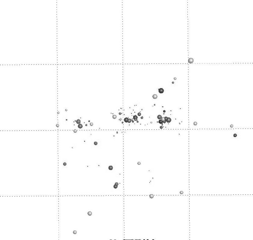
Figure 1: A representation of the Local Volume, looking in the Supergalactic Plane toward $L=90\arcdeg$. Galaxies are shown as spheres with volume proportional to luminosity. In the center is the Local Group; to the left Centaurus, to the right IC 342 and M81/2. The Supergalactic Plane itself is evident, as is the tendency for galaxies to collect in groups. Dotted lines are at 5 Mpc intervals.

The process by which a (nearly) smooth distribution of matter develops present-day structure is complicated, engaging the efforts of many people (and computers). But endpoints, if they can be usefully fixed, by themselves tell something about the process on the average. This study constructs a beginning endpoint for the galaxies in the Local Volume and investigates the consequences of it. (Structure formation by gravitational instability of small perturbations actually starts at recombination, many years after the Big Bang itself; but for our purposes it’s close enough that it may be placed at $t=0$.)

2 Constructing the Beginning

There are two conditions we may impose on the Local Volume at the beginning.

• The motions of the galaxies must be quiet, fitting smoothly onto the general Hubble flow at early times. This condition is imposed, for instance, by Peebles (1989) in his Least Action calculations (and in subsequent studies using similar techniques). It assumes, perhaps implicity, that each body retains some identity all the way back to $t=0$.

• The material out of which the galaxies are made must be smooth, evenly distributed (or with only very small fluctuations) over space. This is a very direct interpretation of measurements of the CMB: radiating matter at the surface of last scattering is observed to have only small deviations from the average. Note that this applies in the first instance to radiating baryonic matter alone; any effects of, or on, dark matter must be inferred.

These conditions are, strictly speaking, inconsistent. The first requires galaxies, or something like them, to exist at the beginning; the second requires that they do not. But a reasonable compromise is possible. We may assume, for the purposes of calculation, that the material out of which a given galaxy is made comes from a simply-connected region at the outset, which may be approximated by a body of the same total mass (or total luminous mass) placed at its centroid. The quality of the approximation will depend on the shape of the region. Strange shapes make it a poor assumption; but very strange shapes seem unlikely. In addition, in their comparison of n-body simulations to the Least Action technique, Dunn & Laflamme (1995) found that the shape of the original region had very little effect on subsequent calculations.

The first condition is dynamic, and implementing it in any practical way would involve us in difficult questions of mass-to-light ratio (and variations thereof with time, mass, and possibly other parameters). The second condition is purely kinematic, much more robust and in fact what we will use for our analysis. It would be convenient to start with the“smooth” condition and forget about quietness; unfortunately, the derivation of an important equation and the algorithm we shall use depend on the dynamical formulation. However, we shall show that, with a trivial substitution, the end points are equivalent. This is worth emphasizing: dynamics is invoked and used at the outset, but the final result we shall apply contains no dynamics at all.

2.1 The Quiet Endpoint: Hubble Equilibrium

Consider the motion of a body $i$ at a position ${\bf r}_{i}$ under the action of $j$ other gravitating bodies of mass $m_{j}$, along with a possible cosmological constant $\Lambda$. Its acceleration is given by

$$\ddot{\bf r}_{i}=G\sum_{j\neq i}m_{j}\frac{{\bf r}_{j}-{\bf r}_{i}}{|{\bf r}_{j}-{\bf r}_{i}|^{3}}+\frac{\Lambda}{3}{\bf r}_{i}$$ (1)

in the nonrelativistic approximation (which holds for the situation of interest to us here). We convert to a different set of coordinates by factoring out a scalar function $a$ which depends only on time, so that ${\bf r}=a{\bf x}$; this gives us

$$\ddot{a}{\bf x}_{i}+2\dot{a}\dot{\bf x}_{i}+a\ddot{\bf x}_{i}=\frac{1}{a^{2}}G\sum_{j\neq i}m_{j}\frac{{\bf x}_{j}-{\bf x}_{i}}{|{\bf x}_{j}-{\bf x}_{i}|^{3}}+a\frac{\Lambda}{3}{\bf x}_{i}$$ (2)

where dots indicate derivatives with respect to time. We are interested in comoving coordinates ${\bf x}$, that is, those which are not functions of time. In that case

$${\bf x}_{i}=\frac{G}{a^{2}\left(\ddot{a}-a\Lambda/3\right)}\sum_{j\neq i}\frac{{\bf x}_{j}-{\bf x}_{i}}{|{\bf x}_{j}-{\bf x}_{i}|^{3}}.$$ (3)

This equation (which may be termed the equation of Hubble equilibrium), when applied at early times, is the mathematical formulation of the quiet condition. The configuration of bodies expands uniformly, at constant comoving coordinates ${\bf x}_{i}$ in an undisturbed Hubble flow. If such a configuration had survived to the present day, it would show no peculiar velocities and no structure other than the bodies themselves.

A thorough study of the solutions to Equation (3) leads to some mathematically interesting results, but most have no obvious application to cosmology. A few are detailed in Whiting (1997). Note that it requires that the expression involving $a$ in the denominator be a constant; this results in the familiar expressions for the universal line-element in (pressureless) Friedmann-Robertson-Walker universes.

To apply the quiet condition to a specific situation, we seek to produce a Hubble equilibrium configuration from a given set of masses at given positions. Now, one may think of the situation described by Equation (3) as an equilibrium between a set of inverse-square, attractive gravitational forces due to the other masses in the universe, and a general repulsive force linear in distance form wherever we take as the center. (Note that this general force is not due to the cosmological constant; it is an artifact of conversion to a non-inertial set of coordinates.) As it stands the equilibrium is unstable: motion toward a given mass makes the attraction to that mass stronger, resulting in more motion toward that mass; moving away makes the gravitational attraction weaker and the general repulsion stronger, increasing motion away. Using even a damped version of the dynamical equations, then, will not find Hubble equilibrium configurations (nor even time-reversed dynamical equations, since it can be shown that Equation (2) has growing modes in either direction).

However, a set of masses at arbitrary coordinates can be relaxed to Hubble equilibrium using the “treacle” method suggested by Lynden-Bell (1995). From the equation of equilibrium (Eq. (3)) construct an effective acceleration

$${\bf A}_{i}={\bf x}_{i}-G\sum_{j\neq i}\frac{{\bf x}_{j}-{\bf x}_{i}}{|{\bf x}_{j}-{\bf x}_{i}|^{3}}$$ (4)

(where various negative constants have been absorbed into $-G$). Since the equilibrium is unstable this effective acceleration must be in a direction away from equilibrium, so if we step each body backwards along this acceleration a small amount, we are getting closer to equilibrium. We may then recalculate the accelerations and iterate again.

It may be useful to think of Hubble relaxation sort of inside-out. In a line of thought attributed to Carlberg (but denied by him, at least in this form), consider that if all forces are reversed, an equilibrium will remain an equilibrium but its stability may change. Thus if the cosmic repulsion of Equation (3) is replaced by a general drawing-in toward the center of the universe and the gravitational attraction by a localized soft repulsion one would still find the same equilibrium. Think of drawing together a number of soft foam balls in a fishing net. This is what the the “treacle” relaxation procedure does.

2.2 The Smooth Endpoint

We now compare the grainy universe of the last section with a completely smooth one. Consider a section of a universe of homogeneous, pressureless fluid of mass density $\rho(t)$. Assuming isotropy, we may determine its dynamics by looking only at a sphere centered on our origin of coordinates. We seek the equation of motion of a point some vector distance ${\bf r}_{i}$ away from the origin. This will be due to the combined gravitational attraction of all the mass in our sphere, plus a cosmological constant if present:

$$\ddot{\bf r}_{i}=G\int\frac{\rho({\bf r}^{\prime})({\bf r}^{\prime}-{\bf r}_{i})}{\left|{\bf r}^{\prime}-{\bf r}_{i}\right|^{3}}d{\bf r}^{\prime}+\frac{\Lambda}{3}{\bf r}_{i}$$ (5)

where the integral must formally be taken over all the sphere. But note that we need only consider the difference between a sphere of matter centered on ${\bf r}_{i}$ (which would exert no net force) and this eccentric sphere centered on the origin, which amounts to an extra shell on one side and a deficit on the other. If the reference sphere is taken to be large enough, these shells can be treated as thin shells at a constant distance.

To remove any explicit dependence on the the details of our coordinate system we consider another point a vector distance ${\bf r}_{j}$ from the origin, opposite ${\bf r}_{i}$, and find

$$\ddot{\bf r}_{i}-\ddot{\bf r}_{j}=G\int\frac{\rho({\bf r}^{\prime})({\bf r}^{\prime}-{\bf r}_{i})}{\left|{\bf r}^{\prime}-{\bf r}_{i}\right|^{3}}d{\bf r}^{\prime}-G\int\frac{\rho({\bf r}^{\prime})({\bf r}^{\prime}-{\bf r}_{j})}{\left|{\bf r}^{\prime}-{\bf r}_{j}\right|^{3}}d{\bf r}^{\prime}+\frac{\Lambda}{3}\left({\bf r}_{i}-{\bf r}_{j}\right).$$ (6)

Now we impose a comoving coordinate system, so that ${\bf r}=a{\bf x}$ and the time derivatives of ${\bf x}$ vanish (that is, the smooth universe is in uniform Hubble-flow expansion); this gives us

$${\bf x}_{i}-{\bf x}_{j}=\frac{G}{\left(\ddot{a}-\Lambda a/3\right)a^{2}}\int\rho({\bf x}^{\prime})\left(\frac{{\bf x}^{\prime}-{\bf x}_{i}}{\left|{\bf x}^{\prime}-{\bf x}_{i}\right|^{3}}-\frac{{\bf x}^{\prime}-{\bf x}_{j}}{\left|{\bf x}^{\prime}-{\bf x}_{j}\right|^{3}}\right)d{\bf x}^{\prime}$$ (7)

where the integral is taken over the appropriate thin shells. Performing these integrals gives the equation of motion for the scale factor:

$$a^{2}\left(\ddot{a}-\frac{\Lambda a}{3}\right)=-\frac{4\pi G}{3}a^{3}\rho$$ (8)

which, if $\rho$ is taken as varying with time in the appropriate way, gives the familiar Friedmann-Robertson-Walker results.

Now we consider, instead of the fluid universe, one in which the mass is concentrated at points, but which is still in Hubble equilibrium; that is, Equation (3) holds for each mass-point. We assume that, on some scale, the discrete universe approaches a constant-density continuous universe, so that we may assign the same $\rho$ to a sufficiently large volume of each. We also assume that the discrete universe approaches isotropy on this same large scale. By applying Equation (3) to the Hubble equilibrium distance between two points we have

$${\bf x}_{i}-{\bf x}_{j}=\frac{G}{\left(\ddot{a}-\Lambda a/3\right)a^{2}}\left(\sum_{k\neq i}m_{k}\frac{{\bf x}_{k}-{\bf x}_{i}}{\left|{\bf x}_{k}-{\bf x}_{i}\right|^{3}}-\sum_{k\neq j}m_{k}\frac{{\bf x}_{k}-{\bf x}_{j}}{\left|{\bf x}_{k}-{\bf x}_{i}\right|^{3}}\right).$$ (9)

Comparing this with Equation (7) we note that the condition of smoothness amounts to each sum approximating the corresponding parts of the integral; and that the fact that the integral need only be taken over thin shells at large distances, means the approximation need only hold at large distances also.

We now seek to compare the gravitational effect of the two Hubble-equilibrium point masses $m_{i}$ and $m_{j}$ on each other with that of the corresponding region in the smooth universe. To isolate the effects we are interested in, let us remove the effects of the distant shells of matter from each universe (smooth and grainy), say by momentarily imposing just the necessary anisotropy. Then, for the discrete case,

$${\bf x}_{i}-{\bf x}_{j}=\frac{G}{\left(\ddot{a}-\Lambda a/3\right)a^{2}}(m_{i}+m_{j})\frac{{\bf x}_{j}-{\bf x}_{i}}{\left|{\bf x}_{j}-{\bf x}_{i}\right|^{3}}.$$ (10)

Now we impose the same behavior of $a$ as in the smooth universe, using Equation (8):

$${\bf x}_{i}-{\bf x}_{j}=\frac{m_{i}+m_{j}}{-4\pi a^{3}\rho/3}\frac{{\bf x}_{i}-{\bf x}_{j}}{\left|{\bf x}_{i}-{\bf x}_{j}\right|^{3}}$$ (11)

that is,

$$\rho=\frac{m_{i}+m_{j}}{4\pi a^{3}\left|{\bf x}_{i}-{\bf x}_{j}\right|^{3}/3}.$$ (12)

So if the two masses are found, one on the center and one on the surface of a sphere of radius $\left|{\bf r}_{i}-{\bf r}_{j}\right|$, as they are in Hubble equilibrium, we recover the behavior of a (dynamically) smooth universe (Equation 8): the masses $m$ are spread out in such a way as to give a constant density, when averaged over any volume containing two or more bodies. (This is much stronger than the earlier assumption of approaching a constant density at large scales.)

2.3 Quiet is also Smooth

Now if we interpret the quantities $m$ in the “treacle” algorithm not as masses, but as luminosities, we find that it allows us to spread out the luminous matter in the smoothest possible way in which the galaxies retain an identity at the beginning. As noted, we have used dynamics only to throw it away at the end.

There are three things to emphasize at this point:

• The “treacle” result is robust, in that very few assumptions are made leading to it. It directly applies the requirement of a smooth distribution of luminous matter.

• The process is not dynamical. How material got from smooth to clumpy is not assumed, inferred or calculated. In particular, the role of dark matter is left quite open.

• The algorithm produces the closest end point (averaged over all the galaxies) to the present configuration. There are very many ways of arranging proto-galactic masses which satisfy Equation (3); it is not contended that “treacle” produces the exact one which led to the structures we now see. In some possible arrangements, the distance a given galaxy travels from the beginning to the end (in some comoving sense, which will be dealt with in detail below) will be smaller; but another galaxy’s distance will be greater. The version calculated here forms an averaged lower limit. (If the Local Volume in fact is dynamically simple, still undergoing infall into the various galaxy groups and the Supergalactic Plane, the “treacle” end point should be close to the actual end point.)

3 Constructing the Final Endpoint

In order to fix the final end point, as well as to start the “treacle” process, we need accurate distances and photometry for all or most of the galaxies within the Volume. We will also be using peculiar velocities, which must be determined from some kinematic model. In what follows we use the data and model of Whiting (2005). References to sources and details of calculations will be found in that paper; here an outline is given.

High-accuracy distances for 149 galaxies were taken from the literature. These are mostly Cepheid and tip of the Red Giant branch (TRGB) distances, with uncertainties of $\sim 10\%$ or better. Another 21 galaxies with distances of lower quality ($\sim 20\%$), but among the brightest, were added. The total of 170 by no means exhausts the total population of the Local Volume, which is estimated to be around 500 (Karachentsev et al., 2004). However, it does include all known galaxies in the Volume brighter than $M_{B}\sim-18.5$, and thus accounts for all but a few percent of the luminosity field. Put another way, all the unincluded dwarfs together would amount to perhaps 2 or 3 giant galaxies of $M_{B}\sim-21$.

There are certainly galaxies hiding behind the plane of the Milky Way which have not found their way into any catalog, and so are not accounted for. One could also consider the possibility of a dark galaxy of the type reported by Minchin et al. (2005), detected (in the Virgo cluster) only in HI radio emission, and so also missing from local galaxy catalogs. But as they note, anything like their discovery within about 6 Mpc would have been detected by the HIPASS survey (which is not blocked by the Galactic plane). It is unlikely that any large galaxy in the Local Volume is missing from our data set. To change the results of this study materially, there would have to be many such objects. (Of course galaxies outside the Volume are not included. Their possible influence is considered below.)

Radial velocities for the galaxy sample were also taken from the literature. Most are HI measurements, with uncertainties of a few km s^-1; a few optical radial velocities, with uncertainties typically of $\sim 10$ km s^-1, are included. (In general, radial velocities are the most accurately determined of the input data.)

From these data an isotropic expansion model was fit by a direct least-squares procedure. The result has the expansion rate of 65.5 km^-1 Mpc^-1 and a motion of the Sun (relative to the average of all galaxies) of 340 km s^-1 in the direction of Galactic longitude $98\arcdeg$, latitude $12\arcdeg$. None of these figures is at great variance with similar determinations. The rms peculiar radial velocity, the deviation from this model, is 79 km s^-1, of which about 8-10 km s^-1 is attributable to distance uncertainties.

It is worth emphasizing that the peculiar velocities thus derived are entirely kinematic. They do not depend on any dynamical model used to describe the overall behavior of the Volume.

Photometric measurements of each galaxy in $B$ and $K$ were sought in the literature. Three galaxies in the sample did not have $B$ photometry; almost two-thirds were missing $K$ measures. In all cases, though, the missing data applied to dwarf galaxies, whose total contribution to the total luminosity is small. The apparent magnitudes were converted to absolute using the known distances.

4 Results and Analysis

The treacle procedure was performed as outlined on the Local Volume data set, and the resulting configuration scaled to be the same average size as the input data. (Since $K$-band luminosities are expected to be more representative of luminous mass than $B$-band, the procedure was run using infrared photometry.) A view of the resulting Hubble equilibrium configuration is shown in Figure (2). The Supergalactic Plane and group structure have been erased, as expected. If we interpret the equation of Hubble equilibrium dynamically (and if $K$ luminosity were exactly proportional to mass) this is one of the possible results if all the Local Volume galaxies had expanded in an undisturbed Hubble Flow. None of these galaxies has any peculiar velocity, nor has any performed any peculiar motion. If we interpret Hubble equilibrium as a kinematic condition on luminous baryons, this configuration spreads them out in the smoothest possible way while each galaxy retains its identity.

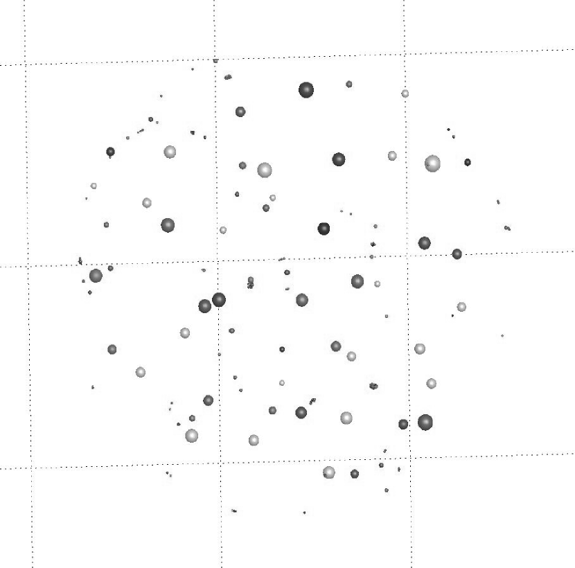
Figure 2: The nearest Hubble equilibrium configuration as found by the “treacle” method for the Local Volume. As in Figure (1), each galaxy is represented by a sphere of volume proportional to luminosity. The even distribution in three dimensions is only hinted at by this two-dimensional view.

To derive any useful or quantitative results from this result, we need to connect the endpoints.

We take, for convenience, the centroid of the Local Volume as the origin. The average motion of a given galaxy from $t=0$ to now is the vector from the origin to its present position, ${\bf r}_{1}$. The average motion it would have followed in the absence of structure formation is the vector from the origin to its position in the Hubble equilibrium configuration, ${\bf r}_{2}$. The average motion required to get from the smooth configuration to the real one is $\Delta{\bf r}={\bf r}_{2}-{\bf r}_{1}$; we may call this the average peculiar motion. (This is not expected to be the actual peculiar motion, which will be curved in some way; but forms a lower bound to it in distance.) To compare computed motions with anything observable we must take radial components, so forming the computed average peculiar radial motion:

$$r_{c}=\Delta{\bf r}\cdot\hat{\bf r}$$ (13)

which, when divided by the age of the universe, gives the computed average peculiar radial velocity. (The terms are clumsy, but it is necessary to be precise.)

A comparison between the calculated peculiar motions and observed peculiar velocities is shown in Figure (3). (Only the 149 galaxies with high-accuracy distances are used, since peculiar velocity uncertainties for the others were much larger.) The solid line gives the relationship one would expect if all galaxies had proceeded directly from their places in the beginning configuration to their present positions at a constant speed over 13.7 Gyr. That is a simplistic idea and it is no surprise at all that the points do not lie on that line.

But there is not even an average monotonic relationship here. Galaxies are as likely to be heading in the wrong direction as not, when compared to the assumption that they came from the nearest smooth Hubble equilibrium configuration. The assumption of dynamical youth, that (apart, perhaps, from the very inner regions) all the galaxy groups in the Local Volume are still experiencing infall and gathering their outlying members from afar, doesn’t appear to be true. In particular, results from the timing argument, whether in its original form by Kahn & Woltjer (1959) or in the zero-velocity surface formulation of Lynden-Bell (1981), must be reexamined (in spite of its continuing popularity, of which van den Bergh (2000) and Karachentsev (2005) are examples). Looked at another way, current peculiar velocities are in the wrong direction to have moved the galaxies of Figure (1) more or less directly from a smooth beginning endpoint.

For further analysis we need to examine the relationship between the computed and observed average speeds.

Figure 3: Peculiar velocity for each body in the 149-galaxy sample of Whiting (2005) plotted against the component of peculiar motion which should show up as radial motion, assuming straight-line motion from the nearest Hubble equilibrium configuration. For an age of the universe of 13.7 Gyr the solid line gives the most direct relation between the two; for 10 Gyr, the dashed line. Present peculiar velocities cannot account for more than about 2 Mpc of peculiar motion.

4.1 Problems with Peculiar Speeds

Leaving aside the matter of roundabout trajectories for the moment, we note that the magnitude of the observed peculiar radial velocities is lower than the required average peculiar radial velocities by a factor of three or more. Of course galaxies did not start with a certain speed on a certain course and proceed thus from the beginning. How should the present observed velocity, $v_{n}$, compare with the average, $\bar{v}$? Consider the following effects:

Nonlinear evolution. Peculiar velocities are not produced from nothing. They come, according to current theory (and there appears to be no viable alternative), from gravitational effects of mass concentrations. We expect these to grow in the course of time, so their effect will be greater at later times. In addition, as objects get closer to each other their gravitational influence will grow (until they pass; see next paragraph). From each of these considerations we expect $v_{n}>\bar{v}$, the opposite of what we see.

Dissipationless collapse. Suppose that, instead of seeing a system in the midst of infall, the components have interacted to the point of virialization. How will the velocities compare?

For a uniform sphere of mass $M$ and total energy $-E$, the radius $r$ during pressureless collapse is given by the parametric equations

$$r = \frac{GM}{E}\sin^{2}(\eta)$$

$$t = \frac{GM}{\sqrt{2}E^{3/2}}\left(\eta-\frac{1}{2}\sin(2\eta)\right)$$

When the radius is just half of maximum, the time elapsed is

$$t_{1/2}=\frac{GM}{\sqrt{2}E^{3/2}}\left(\frac{\pi}{4}+\frac{1}{2}\right)$$ (14)

Though the surface of the sphere has changed its position by half the original radius, most points have not gone so far; the average motion over the volume is 3/8 of the original radius. With this figure and the time above we have the expected average velocity.

Now consider the same sphere, but allow its components to virialize. Then its original total energy at maximum expansion, $-E=3GM^{2}/(5R)$, is distributed among its components such that

$$\frac{1}{2}Mv_{v}^{2}=E$$ (15)

and the virialized radius is half the original one. Comparing the average virialized velocity with the average infall velocity above, we find

$$\frac{v_{v}}{v_{i}}=5.7$$ (16)

So dissipationless collapse will also tend to increase observed velocities.

Dissipational collapse. In order to form galaxies at all, baryonic matter must interact and lose kinetic energy to fall to the center of dark-matter potential wells, so dissipation must act at some point in structure formation. However, when dealing with the whole Local Volume the density of luminous matter is far lower than in galaxies (or protogalaxies). Indeed, since the local Hubble flow is so close to the global value (and the age is the same), the local average density must be close to the global density, which is far too low for gas pressure to have any effect. For dissipation to happen galaxies must come together.

There is dissipation within galaxy groups. Indeed, merging has certainly taken place in the major galaxies (as the remnants of merged satellites show). That does not help with motions on several-Mpc scales, however. To modify peculiar velocities sufficiently we need interactions between galaxy groups, and they are too far away from each other now to have interacted and then reached their present positions at their present speeds.

Possibly one could arrange trajectories so that galaxies coming from very different directions or places preferentially merged, or interacted in some way so as to convert most of their kinetic energy into other forms. This does not seem likely (merging is most probable for objects with similar velocities, not those speeding past each other) and does not appear to be a feature of simulations.

Under expected conditions, then, dissipational collapse should not be an important effect for motions on several-Mpc scales.

The effect of external bodies. The 10 Mpc limit is somewhat arbitrary, set by current observational capabilities (resolved-star distances are very difficult to get at larger distances), not by dynamical or kinematic considerations. There are certainly galaxies beyond the border which have some dynamical effect.

One effect could be to flatten the configuration of Figure (2), which would bring galaxies closer to their present positions in the Supergalactic Plane. This solves only a minor part of the problem, however; there are still gaps in the Plane which cannot be filled at present peculiar velocities. One could imagine placing external galaxies in such a way as to fill in all the holes. But this is terribly contrived, and very unlikely; and would result in some strange peculiar velocity patterns outside the Volume.

External masses could affect peculiar velocities. But even large nearby clusters do not generate the tidal fields of high spatial frequency needed to interfere with Mpc-scale motions. Virgo, for instance, can attract everything in the Volume toward it (monopole effect) and add an ellipsoidal (quadrupole) component to peculiar velocities. But it cannot make a significant change in the infall pattern into, say, the M81/2 group, which is at best 2 Mpc across, from 17 Mpc away. And there does not appear to be an obvious way for an external mass to have a general cooling effect on all peculiar motions.

The decay of peculiar velocity. The peculiar velocity of an object moving freely in an expanding universe decays, slowing down relative to the local coordinate system. As shown, for example, in Peebles (1993), $v\sim 1/a$, where $a$ is the scale factor of the background cosmology. For the simplest background, the critical, lambda-less universe,

$$\frac{\bar{v}}{v_{n}}=\frac{t_{n}^{2/3}}{t_{n}-t_{0}}\int_{t_{0}}^{t_{n}}\frac{dt}{t^{2/3}}$$ (17)

where variables with subscript $n$ denote the values now and subscript 0 the time at which the particle began to propagate. If we take the extreme case of $t_{0}=0$, we get

$$\frac{\bar{v}}{v_{n}}=3$$ (18)

that is, the average speed of a freely-moving particle which starts out at the beginning is three times its present speed. For a flat universe with cosmological constant $\Lambda$ the expression is more complicated,

$$\frac{\bar{v}}{v_{n}}=\frac{\sinh(3\sqrt{\Lambda}t_{n}/2)^{2/3}}{(3\sqrt{\Lambda}/2)(t_{n}-t_{0})}\int_{t_{0}}^{t_{n}}\frac{dt}{\sinh(3\sqrt{\Lambda}t/2)^{2/3}}$$ (19)

but inserting the values appropriate for a 13.7 Gyr universe with a 70 km s^-1 Mpc^-1 Hubble constant we come up with

$$\frac{\bar{v}}{v_{n}}=3.6$$ (20)

(not an enormous difference).

This time we have a present velocity smaller than the average, and a glance at Figure (3) shows it to be apparently the right amount. If the magnitude of the peculiar velocities is increased by a factor of three or four then the 13.7 Gyr line is found among them, not rising far above and falling far below. But there remains a problem: half of the galaxies are still moving in the wrong direction. They will need speeds of several times that shown, in order to go around and come back (speaking roughly). Even though the decay of peculiar velocity acts in the right direction, it’s still not enough to fix the problem.

This is worth emphasizing. By taking a galaxy at $t=0$ (before any had formed) and giving it an initial push (before there was anything to push it), we have given it more than the longest possible time for its peculiar velocity to decay; this is a limit. Even under these conditions, it is not enough.

Bias in the data. The result relies upon galaxy distances reported in the literature. They were chosen for study for a variety of reasons and with no necessary relation to other objects, the opposite of a carefully-constructed survey. In such a situation one expects to encounter bias, at least in the sense that the data used are not strictly representative of the underlying population. In the Local Volume in particular one expects more attention to be paid to brighter galaxies (more interesting because more complicated, having a wider variety of internal features, and of course easier to study). And indeed the galaxies lacking in the sample are mostly small dwarfs.

But the sample does contain a wide range of luminosities, as shown in Figure (4). In addition, a bias in the sample toward bright galaxies seems to make no difference in peculiar velocity; the graphs have a remarkably even distribution.

And even if the Local Volume galaxies missing in the present sample had radically different kinematics it would make no difference to the result, since almost all of the luminosity is accounted for. A few percent additional would not affect the relaxed configuration in any significant way; it might not even be measurable.

Figure 4: Peculiar velocities for the sample of Local Volume galaxies, plotted against (left) absolute magnitude in the $B$ band and (right) absolute magnitude in the $K$ band. Of the 149 galaxies with accurate distances, two did not have $B$ photometry and do not show up on the left; about two-thirds lacked $K$ photometry and do not show up on the right. The missing galaxies are dwarfs, fainter than about -18 in $B$ and -15 in $K$. Apart from an apparent lack of high negative peculiar velocities among giant galaxies in $B$ and a sparsely-populated plot for faint $K$, there are no visible correlations.

To dispose of another red herring, dynamical bias has been reported in cosmological simulations between the general dark matter velocity dispersion and those objects identifiable as galaxies. Diemand et al. (2004) find that it amounts to 10-20%, and so too small to interest us here. More importantly, as noted, Hubble relaxation using luminosity makes no reference to dark matter at all. Any bias between dark and luminous matter is beside the point: the luminous matter by itself is required to be smooth at $t=0$.

In summary, observed peculiar velocities are too small by a factor of at least a few to produce the observed structure in the Local Volume from a smooth distribution at recombination. If we ignore all effects which tend to increase current peculiar velocities relative to the overall time average, and push the one decreasing effect to an unreasonable limit, we still cannot resolve the discrepancy.

Looked at another way, if the structures of Figure (1) are pushed apart at the observed peculiar speeds over 13.7 Gyr, they would still be far from smoothly distributed over the Volume.

5 Comparison with Other Work

5.1 Cold Flow

A point should be emphasized here: the low peculiar velocities referred to here do not consitute the long-standing problem of “cold flow.” As found in the literature, that phrase seems to refer to three slightly different situations:

• Local peculiar velocities of the same size as the observational uncertainties, about 60 km s^-1, so that one could not conclude that there was any departure from uniform expansion. Sandage (1986), for example, makes this point. This problem was in part due to small-number statistics giving a slightly low dispersion and in part due to large observational uncertainties. As noted above, with uncertainties on the 10 km s^-1 level, one can say that 70 km s^-1 of motion is real.

• The discrepancy between simulations (mostly CDM with a critical, lambdaless universe) giving peculiar velocity dispersions near 500 km s^-1 and local determinations one-fifth that size. Going to a different background cosmology seems to have resolved this issue; see, for example, Klypin et al. (2003). But, as noted, the present study makes no dynamical calculations at all, so does not apply to this problem.

• The local velocity dispersion is still small compared with the bulk motion of the whole Local Volume with respect to the CMB, $\sim 600$ km s^-1. Since I have not dealt with motion outside the Volume, there is no direct connection between this “cosmic Mach number” discrepancy and that shown by the Hubble relaxation process.

5.2 N-Body Simulations

Any new result in the area of structure formation prompts a call for comparison with n-body simulations. This is reasonable, given the great success the method has enjoyed in producing results which match observations, especially on large scales. Unfortunately, there is no direct way to compare my procedure with these codes. Some of the assumptions (an expanding background universe, a smooth beginning) are the same; but simulations are dynamical calculations, dealing directly with the process of producing velocities, while Hubble equilibrium (interpreted in the form of baryon luminosity) has nothing to say about dynamics. One cannot compare, for instance, methods of dealing with dark matter, as one can between codes.

5.2.1 Simulating the Local Volume?

There are no doubt ways to make an indirect connection with some suitable simulation of the Local Volume. Unfortunately, such a phrase is something of a misnomer: even if we had all the distance and velocity information to start a backwards integration (which we certainly do not), the process is mathematically unstable at early times, producing the wrong type of infinite motions.

N-body simulations work the other way, starting at some early time and running forward. The output is scrutinized for its resemblence to the observed universe. Overall features can be specified to some degree (Klypin et al., 2003), but in the strict sense no one simulates the Local Volume; one simulates something which shares the important features of the Volume (and what those features are will vary from study to study).

Complicating the problem is the probability of the Volume being, in a dynamical sense, rather unusual. Over large volumes, for instance, the observed rms peculiar velocity is much higher than locally, 400-500 km s^-1 (Hawkins et al., 2003), which one might list as a fourth interpretation of “cold flow”. This means that a simulation might be an accurate picture of the universe in general, containing all the right physics and cosmological input parameters, while still failing to produce something quite like the Local Volume. Along these lines, note that Diemand et al. (2004) simulate the velocity dispersions well in galaxy clusters but poorly (compared to observations) around individual galaxies.

There are also some difficulties in interpreting a simulation in terms of observational data. For instance, a recent simulation of the region around the Milky Way (Macciò et al., 2005) has the right number of dark-matter haloes for large galaxies but far too many for the smaller dwarfs (the venerable “missing satellite” problem). To deal with this kind of situation, the simulation of Benson et al. (2002) implements a relatively sophisticated procedure for converting the characteristics of a dark halo into those of an observable galaxy, but one which they note has its limitations.

So producing a convincing simulation of the Local Volume is difficult. Especially problematic is judging the uncertainties in the procedure, so that one might be able to say that something is indeed ruled out by the calculation. The strategy of this paper is different. Instead of searching for accurate models it seeks to put limits on possible behavior. The results are cruder, but more robust.

5.2.2 Testing Assumptions

There has been one study testing some of the assumptions used in this paper against simulations. Dunn & Laflamme (1995) compared an n-body code with a Least Action reconstruction technique similar to that in Peebles (1989). It was a comparison between dynamical calculations, with results framed in terms of the determined mean density of the region ($\Omega$) in a lambdaless cosmology, and so dealing with different questions than we are here. However, the authors have two results worth noting. First they found that the initial shape of a protogalaxy (the fact that it was not a point mass, as assumed by the Least Action method) had little or no effect on any difference in results. The two calculations did indeed come up with different answers for trajectories and velocities; the authors attributed the difference to “orphan” dark matter particles not included in identified galaxies. As far as that is applicable, it underlines the difficulty in deciding how to choose observables from a given simulation.

5.3 The Baryon Deficit

The main result of this study, that the luminous matter in the Local Volume is moving too slowly to have been smoothly distributed at recombination, has one strightforward explanation for which there is some independent observational evidence. If all the luminous matter in the universe (or a representative part thereof) is counted up, that is everything in stars and stellar remnants, it only makes up a small part of the baryon density required by Big Bang nucleosynthesis. Persic & Salucci (1992) noted the discrepancy and the slightly updated figures of Fukugita, Hogan & Peebles (1998) make stars and remnants 17% of the required baryons, the rest being ionized gas. Suppose such gas is present in the Local Volume in large quantities and distributed differently from galaxies. In particular, if it is found preferentially away from the structures in Figure (1) then the baryons within the structures need not travel so far (in comoving terms); thus it might allow all baryons at recombination to present a smooth front to the world, while allowing galaxies to move to their present positions at a more stately pace.

In principle the gas might be detectable in X-rays, in emission or absorption. Some galaxy groups of quite modest mass (less than 100 km s^-1 dispersion) have an observed X-ray flux (Helsdon, Ponman & Mulchaey, 2005), though none are in the Local Volume, and for those the inferred gas mass fraction is on the order of 10%. It is unclear how much gas would be necessary to explain the peculiar velocity deficit (there is no obvious way to run the “treacle” procedure with an unknown additional field of matter), but certainly it would be several times that of the (visible-light) luminous matter. It might soon be possible to detect much more tenuous material (Yoshikawa et al., 2003).

6 Summary and Conclusions

Imposing an end condition on the visible matter in the Local Volume has revealed a problem with the currently-visible structures: they are moving too slowly and often in the wrong direction for the observed peculiar velocities to have produced them from a smooth distribution at the time of recombination. Setting limits (rather than performing detailed calculations), it has been found that no known dynamical process explains the deficit.

The most straightforward explanation is that much or most of the baryonic matter in the Volume is in the form of ionized gas, or for some other reason not now presently detectable; and that it is distributed largely in the places where galaxies are not. In that case it might be observed soon, as X-ray technology improves.

This is not the only possible explanation, however. Some previously unsuspected way of modifying peculiar velocities might be at work, slowing everything down greatly. This solution, though, is only speculative.

Complicating the interpretation of this result is the fact that the Local Volume is both dynamically unusual and the only region which may be examined in this detail. It is possible that any volume in which the peculiar velocity field can be determined to an accuracy of, say, 20 km s^-1 and sampled to scales of well under one Mpc, will show this kind of anomaly. It is also possible that something is happening here that does not occur in most of the universe.

It is certain, however, that the assumption of simple trajectories for galaxies within the Volume, freely employed up to this time, must be reexamined. It might indeed be a reasonable approximation on some scales and in some cases, but subsequent use of it must be justified.

References

- Benson et al. (2002) Benson, A. J., Frenk, C. S., Lacey, C. G., Baugh, C. M., & Cole, S. 2002, MNRAS, 333, 177
- Diemand et al. (2004) Diemand, J., Moore, B., & Stadel, J. 2004, MNRAS, 352, 535
- Dunn & Laflamme (1995) Dunn, A. M., & Laflamme, R. 1995, ApJ, 443, 1
- Finney (1970) Finney, J. L. 1970, Proc. Royal Soc. London, 319, 479
- Fukugita, Hogan & Peebles (1998) Fukugita, M., Hogan, C. J., & Peebles, P. J. E. 1998, ApJ, 503, 518
- Hawkins et al. (2003) Hawkins, E., et al. 2003, MNRAS, 346, 78
- Helsdon, Ponman & Mulchaey (2005) Helsdon, S. F., Ponman, T. J., & Mulchaey, J. S. 2005, ApJ, 618, 679
- Kahn & Woltjer (1959) Kahn, F. D., & Woltjer, L. 1959, ApJ, 130, 705
- Karachentsev et al. (2004) Karachentsev, I. D., Karachentseva, V. E, Huchtmeier, W. K., & Makarov, D. I. 2004, AJ, 127, 2031
- Karachentsev (2005) Karachentsev, I. D. 2005, AJ, 129, 178
- Klypin et al. (2003) Klypin, A., Hoffman, Y., Kravtsov, A. V., & Gottlöber, S. 2003, ApJ, 596, 19
- Layzer (1963) Layzer, D. 1963, ApJ, 138, 174
- Lynden-Bell (1981) Lynden-Bell, D. L. 1981, Observatory, 101, 111
- Lynden-Bell (1995) Lynden-Bell, D. L. 1995, private communication.
- Macciò et al. (2005) Macciò, A. B., Moore, B., Stadel, J., & Diemand, J. 2005, MNRAS, in press (astro-ph/0506125)
- Minchin et al. (2005) Minchin, R., et al. 2005, ApJ, 622, L21
- Peebles (1989) Peebles, P. J. E. 1989, ApJ, 344, 53
- Peebles (1993) Peebles, P. J. E. 1993, Principles of Physical Cosmology (Princeton: Princeton University Press)
- Persic & Salucci (1992) Persic, M., & Salucci, P. 1992, MNRAS, 258, 14p
- Sandage (1986) Sandage, A. 1986, ApJ, 307, 1
- van den Bergh (2000) van den Bergh, S. 2000, PASP, 112, 529
- Whiting (1997) Whiting, A. B. 1997, PhD thesis, University of Cambridge
- Whiting (2005) Whiting, A. B. 2005, ApJ, 622, 217
- Yoshikawa et al. (2003) Yoshikawa, K., et al. 2003, PASJ, 55, 879