Nonaxisymmetric Magnetorotational Instability in Proto-Neutron Stars

Abstract

We investigate the stability of differentially rotating proto-neutron stars (PNSs) with a toroidal magnetic field. Stability criteria for nonaxisymmetric MHD instabilities are derived using a local linear analysis. PNSs are expected to have much stronger radial shear in the rotation velocity compared to normal stars. We find that nonaxisymmetric magnetorotational instability (NMRI) with a large azimuthal wavenumber $m$ is dominant over the kink mode ($m=1$) in differentially rotating PNSs. The growth rate of the NMRI is of the order of the angular velocity $\Omega$ which is faster than that of the kink-type instability by several orders of magnitude. The stability criteria are analogous to those of the axisymmetric magnetorotational instability with a poloidal field, although the effects of leptonic gradients are considered in our analysis. The NMRI can grow even in convectively stable layers if the wavevectors of unstable modes are parallel to the restoring force by the Brunt-Väisälä oscillation. The nonlinear evolution of NMRI could amplify the magnetic fields and drive MHD turbulence in PNSs, which may lead to enhancement of the neutrino luminosity.

1 INTRODUCTION

Neutron stars are formed in the aftermath of supernova explosions associated to the gravitational core-collapse of massive stars (8 – $30M_{\sun}$) at the end of their evolutions. The binding energies released by core-collapse are stored in the interior of a newly born hot neutron star, and those energies are emitted as the neutrinos in the explosion stage. Neutrino emission from proto-neutron stars (PNSs) is one of the key processes of the delayed explosion scenario of core-collapse supernovae, in other words, the size of neutrino luminosities and the energy deposition efficiency determine whether the explosion will succeed or not (Bethe 1990).

Convection in PNSs is considered to play an important role in enhancing the neutrino luminosities (Epstein 1979; Lattimer & Mazurek 1981; Arnett 1987; Burrows & Lattimer 1986; Burrow & Fryxell 1993). Other hydrodynamic instabilities may also contribute to the enhancement of neutrino luminosities (Bruenn & Dineva 1996; Mezzaacappa et al. 1998a; Miralles et al. 2000, 2002, 2004). Mayle (1985) and Wilson & Mayle (1988, 1993) have argued that the material in the PNSs would be unstable to a double diffusive instability which is referred to as “neutron finger”. Bruenn et al. (2004) have found a new double diffusive instability called “lepto-entropy finger instability”. However, despite considering various hydrodynamic instabilities, recent numerical simulations have not succeeded in producing sufficient neutrino luminosities leading to the delayed supernova explosions (Burrows et al. 1993; Keil et al. 1996; Mezzacappa et al. 1998b; Buras et al. 2003).

One of the primary causes of the inefficient neutrino luminosity is the strong radial gradients of the entropy and leptonic fraction. Stable stratification of these quantities appears at the outer layer of PNSs and suppresses convective motions (Janka & Müller 1996). Convective regions are located deep inside of PNSs and surrounded by a convectively stable layer in which the surface fluxes of $\nu_{e}$ and $\tilde{\nu_{e}}$ are mainly built up (Buras et al. 2003). Thus the convection in PNS has little influence on the emission of neutrinos and is irrelevant for the supernova dynamics.

On the other hand, MHD instabilities could be a seed of turbulence even in the stably stratified layer. Magnetic effects on the dynamics of supernovae have been examined actively since the importance of magnetorotational instability (MRI) in supernova cores is pointed out (Akiyama et al. 2003). Two-dimensional MHD simulations of the collapse of supernova cores indicate that the shapes of shock waves and the neutrino sphere can be modified by the effects of magnetic fields (Kotake et al. 2004; Yamada & Sawai 2004; Takiwaki et al. 2004). Thompson et al. (2005) suggest that the turbulent viscosities sustained by the MRI convert the rotational energies of supernova core into the thermal energies and may affect the supernova dynamics. However, effects of magnetic phenomena inside of the PNSs have not been understood yet and still have many uncertainties.

Therefore, in this paper we analyze the linear growth of MHD instabilities in the stably stratified layer of PNSs, and discuss the possibility of enhancement of neutrino luminosities. Especially, we focus on the instabilities caused by a strong differential rotation. We assume the toroidal component of the field is dominant in the supernova cores. Local stability of stellar objects with a rotation and toroidal magnetic fields have been investigated by many authors (Fricke 1969; Tayler 1973; Acheson 1978; Pitts & Tayler 1985; Schmitt & Rosner 1986; Spruit 1999, 2002). Spruit (1999) concluded that the kink-type instability (Tayler instability) grows at first among various MHD instabilities in stellar radiative zone. However, most of the previous work assume a weak differential rotation because their motivation is for the interiors of main sequence stars like the Sun. The stability analysis for the cases of a strong differential rotation, which is expected in PNSs, has not been carried out sufficiently. In such cases, nonaxisymmetric magnetorotational instability (NMRI) could be dominant over the kink-type instability (Balbus & Hawley 1992). The nonlinear evolutions of the NMRI can initiate and sustain MHD turbulence and amplify magnetic fields, which may lead to the enhancement of neutrino luminosity via magnetoconvection, viscous heating, and the other MHD phenomena.

The paper is organized as follows. In §2 we obtain the dispersion equation that determines the stability of PNSs. In §3 we discuss the general properties of the dispersion relation, and in §4 stability criteria and the maximum growth rate are derived by an analytical approach. In §5 we apply our results to the interiors of PNSs, and examine the linear growth of MHD instabilities. The conditions that the NMRI can be dominant over the kink-type instability and the nonlinear effects of MHD instabilities are discussed in §6. Finally, we summarize our main findings in §7.

2 THE DISPERSION RELATION

We examine the stability of PNSs with a toroidal magnetic field using a linear perturbation theory. Acheson (1978) obtained a local dispersion equation for MHD instabilities in stellar objects with a toroidal field. We derive our dispersion equation following Acheson’s analysis. One of the original features of this work is that we consider the effects of leptonic gradients which can be important in PNSs. The size of differential rotation in PNSs could be much larger than that in other stellar objects (Villain et al. 2004). Therefore we focus on the cases of a strong differential rotation which are not well studied in previous work.

The leptonization and cooling timescales of PNSs are much longer than the growth time of the instabilities considered in this paper. Thus the unperturbed state can be treated in a quasi-stationary approximation. The conductivity of plasma inside PNSs is so large that the decay timescale of magnetic fields is much longer than their cooling time. Then, the governing equations are the ideal MHD equations;

$${\frac{\partial\rho}{\partial t}}+\nabla\cdot(\rho\mbox{\boldmath$u$})=0\;,$$ (1)

$${\frac{\partial\mbox{\boldmath$u$}}{\partial t}}+(\mbox{\boldmath$u$}\cdot\nabla)\mbox{\boldmath$u$}=-\frac{1}{\rho}\nabla\left(p+\frac{1}{2\mu}\mbox{\boldmath$B$}^{2}\right)+\frac{1}{\rho}(\mbox{\boldmath$B$}\cdot\nabla)\mbox{\boldmath$B$}+\mbox{\boldmath$g$}\;,$$ (2)

$${\frac{\partial\mbox{\boldmath$B$}}{\partial t}}=\nabla\times(\mbox{\boldmath$u$}\times\mbox{\boldmath$B$})\;,$$ (3)

where $\rho$ is the mass density, $u$ is the fluid velocity, $p$ is the pressure, $B$ is the magnetic field, $g$ is the gravity, and $\mu$ is the magnetic permeability.

We use the cylindrical coordinates $(r,\phi,z)$, and consider the Eulerian perturbations (denoted by a prefix $\delta$) with the WKB spatial and temporal dependence, $\delta\propto\exp\{i(k_{r}r+m\phi+k_{z}z-\sigma t)\}$. Our analysis is purely local one, formally valid only in the immediate neighborhood of a particular location $(r,z)$ and then only for perturbations of wavelength $\lambda$ in the $r$-$z$ plane such that $\lambda^{2}\ll r^{2}+z^{2}$. The azimuthal wavelength can be quite large, perhaps order of radius.

Let us consider a PNS rotating with the angular velocity $\Omega$ and toroidal magnetic fields $B_{\phi}$. We assume these variables depend only on $r$ and have a power-law dependence; $\Omega(r)\propto r^{-q}$ and $B_{\phi}(r)\propto r^{-s}$. At the unperturbed state, the PNS is in the magneto-hydrostatic equilibrium, that is,

$${\frac{B_{\phi}^{2}}{\mu\rho r}}+\displaystyle{\frac{1}{\rho}}\displaystyle{\frac{\partial p}{\partial r}}+\displaystyle{\frac{B_{\phi}}{\mu\rho}}\displaystyle{\frac{\partial B_{\phi}}{\partial r}}=-g_{r}+r\Omega^{2}\;,$$ (4)

$$\vbox{\kern 20.0pt}\displaystyle{\frac{1}{\rho}}\displaystyle{\frac{\partial p}{\partial z}}=-g_{z}\;,$$ (5)

in the radial and vertical directions, respectively.

When written out in component form and only the largest terms retained, the above set of equations becomes to linear order ;

$$k_{r}\delta u_{r}+k_{z}\delta u_{z}=0\;,$$ (6)

$$i\omega\delta u_{r}+2\Omega\delta u_{\phi}+\displaystyle{\frac{imB_{\phi}}{\mu\rho r}}\delta b_{r}=\displaystyle{\frac{ik_{r}}{\rho}}\delta p+\displaystyle{\frac{B_{\phi}}{\mu\rho r}}(2+ik_{r}r)\delta b_{\phi}+\displaystyle{\frac{\delta\rho}{\rho}}g_{r}^{*}\;,$$ (7)

$$i\omega\delta u_{\phi}-(2-q)\Omega\delta u_{r}=-(1-s)\displaystyle{\frac{B_{\phi}}{\mu\rho r}}\delta b_{r}+\displaystyle{\frac{im}{\rho r}}\delta p\;,$$ (8)

$$i\omega\delta u_{z}+\displaystyle{\frac{imB_{\phi}}{\mu\rho r}}\delta B_{z}=\displaystyle{\frac{ik_{z}}{\rho}}\delta p+\displaystyle{\frac{ik_{z}B_{\phi}}{\mu\rho}}\delta b_{\phi}+\displaystyle{\frac{\delta\rho}{\rho}}g_{z}^{*}\;,$$ (9)

$$\omega\delta b_{r}=-\displaystyle{\frac{mB_{\phi}}{r}}\delta u_{r}\;,$$ (10)

$$i\omega\delta b_{\phi}+(1+s)\displaystyle{\frac{B_{\phi}}{r}}\delta u_{r}=q\Omega\delta b_{r}-\displaystyle{\frac{imB_{\phi}}{r}}\delta u_{\phi}\;,$$ (11)

$$\omega\delta b_{z}=-\displaystyle{\frac{mB_{\phi}}{r}}\delta u_{z}\;,$$ (12)

where

$$\omega=\sigma-m\Omega\;,$$

$$\mbox{\boldmath$g$}^{*}=(-g_{r}^{*},-g_{z}^{*})=(-g_{r}+r\Omega^{2},-g_{z})\;.$$

Here we assume the local approximation $(k\gg 1/r,m/r)$. We also adopt the Boussinesq approximation (e.g., Chandrasekhar 1961) because the Alfv́en speed and the rotation velocity of PNSs would be much smaller than the sound speed $c_{s}\simeq 0.1c$ where $c$ is the speed of light. In addition to these linearized equations, we use a relation by virtue of the local approximation, $\delta p+B_{\phi}\delta b_{\phi}/\mu=0$. This relation means that a fluctuation of the total pressure is negligible (Acheson 1978).

To complete our set, we require another linearized equation. The chemical equilibrium is realized in PNSs, and thus the density is given by a function of pressure $p$, temperature $T$, and leptonic fraction $Y_{l}=(n_{e}+n_{\nu})/n$ where $n_{e}$, $n_{\nu}$, and $n$ are the number densities of electrons, neutrinos, and baryons, respectively. In the Boussinesq approximation, the pressure perturbations are negligible because fluid elements are assumed to be moving slowly and in the pressure equilibrium with their surroundings. Then, the perturbations of density $\delta\rho$ and entropy per baryon $\delta S$ can be expressed in terms of the perturbations of temperature $\delta T$ and leptonic fraction $\delta Y_{l}$:

$$\delta\rho=-\rho\Big{(}\alpha\displaystyle{\frac{\delta T}{T}+\xi\delta Y_{l}}\Big{)}\;,$$ (13)

$$\delta S=m_{B}c_{p}\displaystyle{\frac{\delta T}{T}}+\zeta\delta Y_{l}\;,$$ (14)

where $m_{B}$ is the baryon mass, $\alpha=-(\partial\ln\rho/\partial\ln T)_{pY_{l}}$, $\xi=-(\partial\ln\rho/\partial Y_{l})_{pT}$ are the coefficients of thermal and chemical expansion, and $c_{p}=(T/m_{B})(\partial S/\partial T)_{pY_{l}}$ is the specific heat at constant pressure. The sign of $\zeta=(\partial S/\partial Y_{l})_{pT}$ determines whether the leptonic gradient is stabilizing or destabilizing. Here we neglect the effects of thermal and chemical diffusions for simplicity. The role of these diffusive processes on the growth of MHD instabilities is discussed later in § 6.1. The equations governing the thermal balance and the diffusion of leptonic fraction are written as

$${\frac{\partial S}{\partial t}}+\mbox{\boldmath$u$}\cdot\nabla S=0\;,$$ (15)

$${\frac{\partial Y_{l}}{\partial t}}+\mbox{\boldmath$u$}\cdot\nabla Y_{l}=0\;,$$ (16)

(Miralles et al. 2004) and then the linearized equations are given by

$$-i\omega\delta T-\delta\mbox{\boldmath$u$}\cdot\left[\left(\displaystyle{\frac{\partial T}{\partial p}}\right)_{s,Y_{l}}\nabla p-\nabla T\right]=0\;,$$ (17)

$$-i\omega\delta Y_{l}+\delta\mbox{\boldmath$u$}\cdot\nabla Y_{l}=0\;.$$ (18)

Substituting equations (17) and (18) into equation (13), we obtain the linearized equation,

$$i\omega\displaystyle{\frac{\delta\rho}{\rho}}+\delta\mbox{\boldmath$u$}\cdot\nabla\Psi=0\;,$$ (19)

where

$$\nabla\Psi=-\displaystyle{\frac{\alpha}{T}}\left[\Big{(}\displaystyle{\frac{\partial T}{\partial p}}\Big{)}_{s,Y_{l}}\nabla p-\nabla T\right]+\xi\nabla Y_{l}\;.$$ (20)

Eliminating perturbed quantities in eight linearized equations [eqs. (6) – (12) and (19)], we obtain the following fourth-order dispersion equation,

$$\displaystyle{\frac{k^{2}}{k^{2}_{z}}}\omega^{4}-\left[2(1+s)\omega^{2}_{A}+\kappa^{2}+2{\frac{k^{2}}{k^{2}_{z}}}m^{2}\omega^{2}_{A}+\displaystyle{\frac{k^{2}}{k^{2}_{z}}}\mbox{\boldmath$G$}\cdot\nabla\Psi\right]\omega^{2}-8m\omega^{2}_{A}\Omega\omega$$

$$-m^{2}\omega^{2}_{A}\left[2q\Omega^{2}+2(1-s)\omega^{2}_{A}-{\frac{k^{2}}{k^{2}_{z}}}m^{2}\omega^{2}_{A}-\displaystyle{\frac{k^{2}}{k^{2}_{z}}}\mbox{\boldmath$G$}\cdot\nabla\Psi\right]=0\;,$$ (21)

where

$$k^{2}=k^{2}_{r}+k^{2}_{z}\;,$$

$$\kappa^{2}=2(2-q)\Omega^{2}=\displaystyle{\frac{1}{r^{3}}}{\frac{\partial(r^{2}\Omega)^{2}}{\partial r}}\;,$$

$$\omega_{A}=\displaystyle{\frac{B_{\phi}}{\sqrt{\mu\rho}r}}=\displaystyle{\frac{v_{A\phi}}{r}}\;,$$

and

$$\mbox{\boldmath$G$}=\mbox{\boldmath$g$}^{*}-\mbox{\boldmath$k$}(\mbox{\boldmath$k$}\cdot\mbox{\boldmath$g$}^{*})/k^{2}\;,$$ (22)

are the square of a poloidal wavenumber, the square of the epicyclic frequency, the Alfén frequency, and the effective gravity vector. When we assume that isobaric and isochoric surfaces coincide, the dispersion equation (21) is simplified further by noting that

$$\mbox{\boldmath$g$}^{*}\times\nabla\Psi=g_{r}^{*}\nabla_{z}\Psi-g_{z}^{*}\nabla_{r}\Psi=0\;.$$ (23)

Then, defining $N^{2}_{r}=g^{*}_{r}\nabla_{r}\Psi$ with an analogous expression for $N^{2}_{z}$, the final form of the dispersion equation becomes,

$$\displaystyle{\frac{k^{2}}{k^{2}_{z}}}\omega^{4}-\left[2(1+s)\omega^{2}_{A}+\kappa^{2}+2{\frac{k^{2}}{k^{2}_{z}}}m^{2}\omega^{2}_{A}+N^{2}_{e}\right]\omega^{2}-8m\omega^{2}_{A}\Omega\omega$$

$$-2qm^{2}\omega^{2}_{A}\Omega^{2}-2(1-s)m^{2}\omega^{4}_{A}+{\frac{k^{2}}{k^{2}_{z}}}m^{4}\omega^{4}_{A}+m^{2}\omega^{2}_{A}N^{2}_{e}=0\;,$$ (24)

where

$$N^{2}_{e}=\left(N_{r}-\displaystyle{\frac{k_{r}}{k_{z}}}N_{z}\right)^{2}\;.$$

The quantities $N_{r}$ and $N_{z}$ are components of the Brunt-Väisälä frequency $N=(\mbox{\boldmath$g$}^{*}\cdot\nabla\Psi)^{1/2}$. As the leptonic gradient is considered here, the Brunt-Väisälä frequency is divided into the thermal buoyancy frequency $N_{T}$ and the leptonic buoyancy frequency $N_{Y_{l}}$;

$$N^{2}=N^{2}_{T}+N^{2}_{Y_{l}}\;,$$ (25)

where

$$N^{2}_{T}=-\displaystyle{\frac{\alpha\mbox{\boldmath$g$}^{*}}{T}}\cdot\left[\left(\displaystyle{\frac{\partial T}{\partial p}}\right)_{s,Y_{l}}\nabla p-\nabla T\right],\ \ \ \ \ N^{2}_{Y_{l}}=\mbox{\boldmath$g$}^{*}\cdot\xi\nabla Y_{l}\;.$$ (26)

If the leptonic gradient is ignored, the dispersion equation (24) is identical to that obtained by Acheson (1978) in the incompressible limit ($c_{s}\to\infty$). There are two physical branches to the dispersion equation: An internal gravity wave branch which is present in the absence of magnetic fields, and an Alfvén wave branch which becomes unstable at sufficiently long azimuthal wavelengths when magnetic fields are present.

Notice that the local analysis is irrelevant in the case that the growth rate of unstable modes is smaller than the differential rotation rate $|d\Omega/d\ln r|=q\Omega$. In that case, this problem should be treated as an initial-value problem (Balbus & Hawley 1992; Kim & Ostriker 2000). This is because nonaxisymmetric disturbances cannot have a simple plane waveform in the presence of the shearing background on the wave crests (Goldreich & Lynden-Bell 1965). In this paper, we focus mainly on the NMRI for strong shear cases ($q\sim 1$) of which the growth rate is comparable to the angular velocity and use the local dispersion equation (24) for the stability analysis for simplicity. Kim & Ostriker (2000) examine the linear growth of the NMRI using both the local WKB analysis and direct integration of the linearized shearing-sheet equations taking account of the time-dependence of the radial wavenumber. They found that the instantenious growth rate in the direct integration is in good agreement with the WKB dispersion relation. The advantage of the simple WKB analysis is that we can derive analytical formula of the stability criteria and the growth rate of the instabilities. In fact, the stability conditions obtained by the WKB dispersion equation for a case of weak differential rotation (Acheson 1978) are quite useful and applied to the recent studies of the evolution of massive stars (Spruit 1999; Heger et al. 2005).

3 GENERAL FEATURES OF THE DISPERSION RELATION

In this section we solve the dispersion equation derived in the previous section and examine the characteristics of MHD instabilities in PNSs. There are four important parameters in the dispersion equation (24): the shear parameter $q$, the Brunt-Väisälä frequency $N$, the ratio between the angular velocity and the Alfvén frequency $\Omega/\omega_{A}$, and the power index of the field distribution $s$. The nature of MHD instabilities, such as the growth rate and characteristic wavelength, depends on these parameters, especially on the shear parameter $q$ and the Brunt-Väisälä frequency $N$.

The shear parameter is quite small in the Sun where the kink instability would be dominant among MHD instabilities (Spruit 1999). However the shear parameter can be of the order of unity in PNSs. In that case, the magnetorotational instability (MRI) can be important as is in rotationally supported accretion disks (e.g., Balbus & Hawley 1998). The growth rate of the MRI could be faster than that of the kink instability by many orders. MHD turbulence generated by the MRI can transport angular momentum inside of PNSs, which may affect their dynamical evolutions.

In stably stratified regions, the Brunt-Väisälä frequency $N$ is real and denotes the size of the negative buoyancy. When $N$ is large, the growth of the axisymmetric MRI is suppressed significantly because the Brunt-Väisälä oscillation prevents the radial motion of fluids (Balbus & Hawley 1994). If the field is purely azimuthal, axisymmetiric modes are stable for the MRI and only nonaxisymmetric modes can be unstable. The nonaxisymmetric MRI (NMRI) in accretion disks has been examined (Balbus & Hawley 1992; Terquem & Papaloizou 1996; Kim & Ostriker 2000) and the operating mechanism is described in detail by Kim & Ostriker (2000). In this paper we investigate the stabilizing effects of $N$ on the growth of the NMRI.

In what follows, we fix the values of the other two parameters. The ratio of angular velocity to the Alfvén frequency and the field distribution are assumed to be $\Omega/\omega_{A}=30$ and $s=-2$, respectively. These are about their typical values in rotating PNSs (see § 5).

3.1 Effects of the Shear Parameter

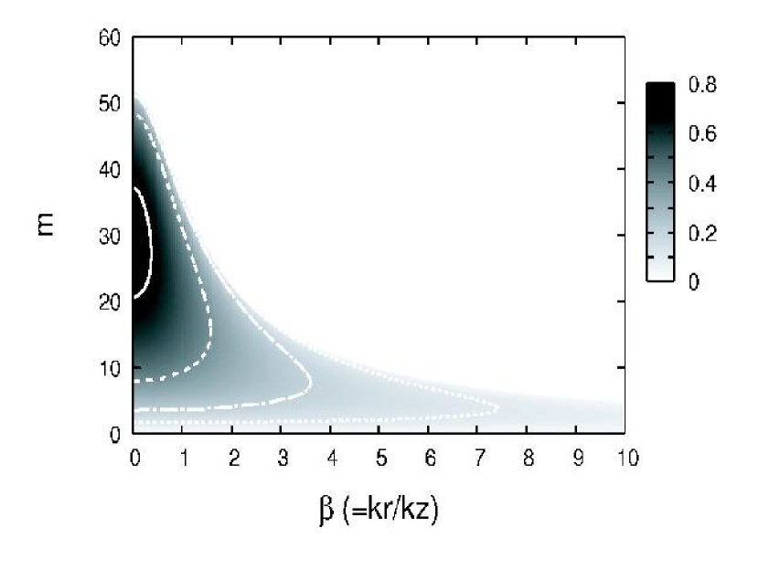
Figure 1: The unstable growth rate $\gamma\equiv\Im(\omega)$ is plotted by the gray contour on the $m$-$\beta$ plane, where $m$ is the azimuthal wavenumber and $\beta\equiv k_{r}/k_{z}$ denotes the ratio of the poloidal wavenumbers. The growth rate is normalized by the angular velocity $\Omega$. Three contour lines indicate $\gamma/\Omega=0.7$ (solid curve), 0.4 (dashed curve), and 0.2 (dot-dashed curve). In this figure, we assume the shear parameter $q=1.5$, the Brunt-Väisälä frequency $N=0$, the ratio of the angular velocity to the Alfvén frequency $\Omega/\omega_{A}=30$, and the field distribution $s=-2$.

First we show the dependence of the growth rate of an unstable branch on the shear parameter $q$. The unstable growth rate is given by the imaginary part of $\omega$, i.e., $\gamma\equiv\Im(\omega)$. In this subsection, the Brunt-Väisälä frequency is assumed to be $N=0$. Figure 1 is a contour plot of the growth rate $\gamma$ for a strong differential rotation case with $q=1.5$. The growth rate is shown as a function of the azimuthal wavenumber $m$ and the ratio of poloidal wavenumbers $\beta\equiv k_{r}/k_{z}$. In this figure, the azimuthal wavenumbers are treated as real values instead of integer. As is expected, the NMRI modes can be seen for this case and the unstable growth rate is of the order of the angular velocity $\Omega$. The maximum growth rate is $\gamma_{\rm{max}}\approx 0.75\Omega$ at $\beta=0$ and $m=29$. For a given $m$, the growth rate takes the maximum at $\beta=0$. The modes with a larger azimuthal wavenumber are stabilized with increasing $\beta$. When $k_{r}\neq 0$, the radial displacements of perturbations lead to undulations of the magnetic pressure, which acts as a stabilizing force for NMRI. Only when $m$ is small there exists unstable modes with a larger $\beta\gg 1$, although the growth rate is much smaller than $\Omega$.

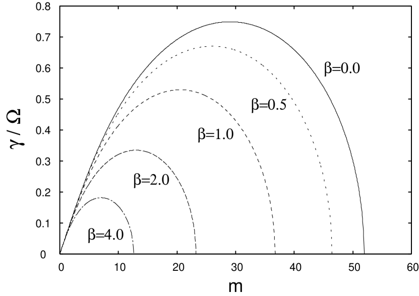
Figure 2: The unstable growth rate $\gamma/\Omega$ as a function of the azimuthal wavenumber $m$. Each lines are labeled by the ratio of the poloidal wavenumbers $\beta$. Model parameters are the same as those in Figure 1.

Figure 2 shows the growth rate $\gamma$ as a function of the azimuthal wavenumber $m$ for $\beta=0$, 0.5, 1, 2, and 4. Model parameters are the same as those in Figure 1. The shape of the dispersion relation is quite similar to that of the axisymmetric MRI (Balbus & Hawley 1991). For a given $\beta$, unstable modes exist when the azimuthal wavenumber $m$ is smaller than a critical value $m_{\rm crit}$ and the growth rate takes the maximum at $m_{\rm{max}}$. These characteristic wavenumbers and the maximum growth rate decreases as $\beta$ increases. When $\beta=0$, the critical and the most unstable wavenumbers are $m_{\rm{crit}}=51$ and $m_{\rm{max}}=29$, respectively.

It would be helpful to recall the axisymmetric MRI to understand the physical meanings of the characteristic values $m_{\rm{max}}$, $m_{\rm{crit}}$, and $\gamma_{\rm{max}}$ shown in Figures 1 and 2. The vertical wavenumber of the fastest growing mode $k_{\rm{max}}$ and the critical wavenumber $k_{\rm{crit}}$ for the axisymmetric MRI are given by $k_{\rm{max}}=\sqrt{-q^{2}+4q}\ \Omega/2v_{\rm{A}}$ and $k_{\rm{crit}}=\sqrt{2q}\ \Omega/v_{\rm{A}}$, and the maximum growth rate is $\gamma_{\rm{max}}=q\Omega/2$ (Balbus & Hawley 1991). When the vertical wavenumber $k$ is replaced by $m/r$, we can estimate the azimuthal wavenumbers $m_{\rm{max}}=\sqrt{-q^{2}+4q}\ \Omega/2\omega_{\rm{A}}\approx 29$ and $m_{\rm{crit}}=\sqrt{2q}\ \Omega/\omega_{\rm{A}}\approx 51$ for $q=1.5$ and $\Omega/\omega_{A}=30$. The maximum growth rate is given by $\gamma_{\rm{max}}=q\Omega/2=0.75\Omega$ for $q=1.5$. These values are exactly consistent with those derived from our dispersion equation (24).

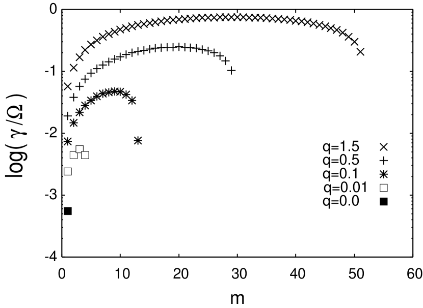
Figure 3: The dependence of the growth rate on the shear parameter $q$. The growth rate is shown as a function of the azimuthal wavenumber $m$ for the cases of $q$ = 1.5, 0.5, 0.1, 0.01, and 0. The poloidal wavenumber is assumed to be $\beta=0$. The other parameters are the same as in Figure 1. The growth rate decreases as the shear parameter decreases. Only the $m=1$ mode can be unstable for the rigid rotation case ($q=0$).

Figure 3 shows the growth rate $\gamma$ as a function of the azimuthal wavenumber $m$ for the cases with different shear parameters $q=0$, 0.01, 0.1, 0.5, and 1.5. The Brunt-Väisälä frequency and the poloidal wavenumber are assumed to be $N=0$ and $\beta=0$. As seen from this figure, the growth rate of NMRI decreases as the shear parameter $q$ decreases. When $q\sim 1$, the growth rate is comparable to the angular velocity. However, if $q$ is less than unity, the maximum growth rate is almost proportional to $q$. The characteristic wavenumber $m_{\max}$ becomes smaller as the shear is weaker. When $q\lesssim 10^{-3}$, only $m=1$ mode is unstable and the the growth rate is about $10^{-3}\Omega$. As is described above, the maximum growth rate of axisymmetric MRI is proportional to $q$, and thus it reaches to zero at $q=0$. However nonaxisymmetric $m=1$ mode is still unstable even for the rigid rotation case ($q=0$). This is quite different from the axisymmetric case and a unique feature of the NMRI.

3.2 Kink-type (Tayler) instability

The stability of the system with a toroidal magnetic field and a weak differential rotation is investigated by many authors (Tayler 1973; Acheson 1978; Schmitt & Rosner 1983; Pitts & Tayler 1986). They found that the kink-type instability ($m=1$) would be important in rigidly rotating stellar interior. The instability criterion for the $m\neq 0$ mode depends on the radial distribution of the field, $s=-d\ln B_{\phi}/d\ln r$ (Spruit 1999). The condition for the instability is given by

$$s<-\frac{m^{2}}{2}-1\;.$$ (27)

Obviously the kink mode ($m=1$) is unstable when $s=-2$. By comparison, the instability criterion for the pinch mode ($m=0$) is given by

$$s<-\displaystyle{\frac{1}{2}}\left(\frac{\Omega}{\omega_{A}}\right)^{2}-1\;.$$ (28)

The pinch mode ($m=0$) is usually stable in rigidly rotating stellar interiors if $\Omega\gg\omega_{A}$.

The growth rate of the kink-type instability is of the order of $\omega^{2}_{A}/\Omega$ (Spruit 1999), which is about $10^{-3}\Omega$ for the case of $\Omega/\omega_{A}=30$. Thus the unstable mode in the limit of $q\rightarrow 0$ shown in Figure 3 must be the kink-type instability. Notice that the NMRI and kink-type instability are on the same branch of the dispersion equation and the kink-type instability corresponds to an asymptotic solution of the NMRI in the limit of the rigid rotation ($q\rightarrow 0$). The growth rate of the kink-type instability is much smaller than that of the NMRI in PNSs with a strong differential rotation, so that it would be anticipated that the NMRI would be dominant there.

Hereafter, we describe the unstable modes with $m=1$ as ”kink modes” in distinction from ”NMRI modes” of $m\geq 2$. The marginal shear rate is estimated by using typical growth rates of the NMRI modes ($\sim q\Omega$) and the kink modes ($\sim\omega^{2}_{A}/\Omega$). From the comparison of these growth rates, we can easily find that NMRI modes are dominant in the strong differential rotation cases $q\gg(\omega_{A}/\Omega)^{2}$, while the kink modes are dominant in the weak differential rotation cases $q\ll(\omega_{A}/\Omega)^{2}$.

3.3 Effects of the Brunt-Väisälä Frequency

In this subsection, we investigate the effects of the Brunt-Väisälä frequency $N$ on the NMRI and kink modes. The Brunt-Väisälä frequency $N$ is real at stably stratified regions. The restoring force acts on displaced fluid elements along the direction of the entropy and leptonic gradients $N$, which is usually toward the center of the star. Using a polar angle $\theta\equiv\tan^{-1}(r/z)$, the radial and vertical components of the Brunt-Väisälä frequency are written as

$$N_{r}=N\sin\theta,\kern 15.0ptN_{z}=N\cos\theta\;.$$ (29)

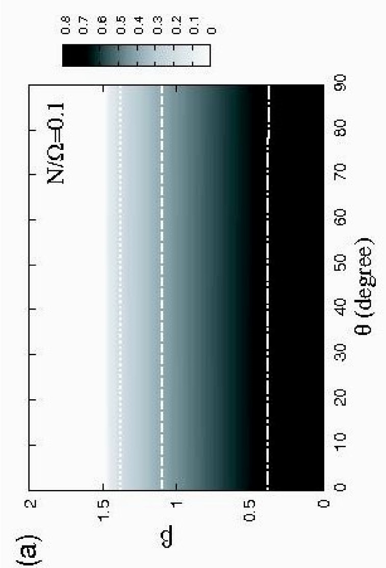
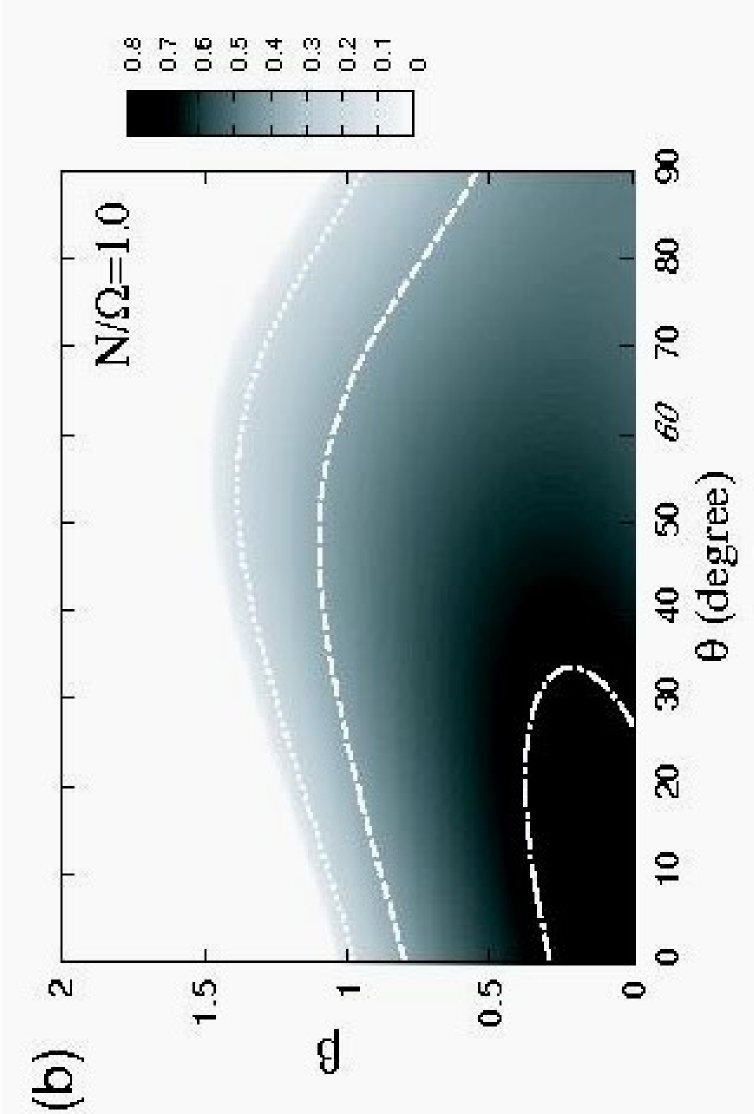
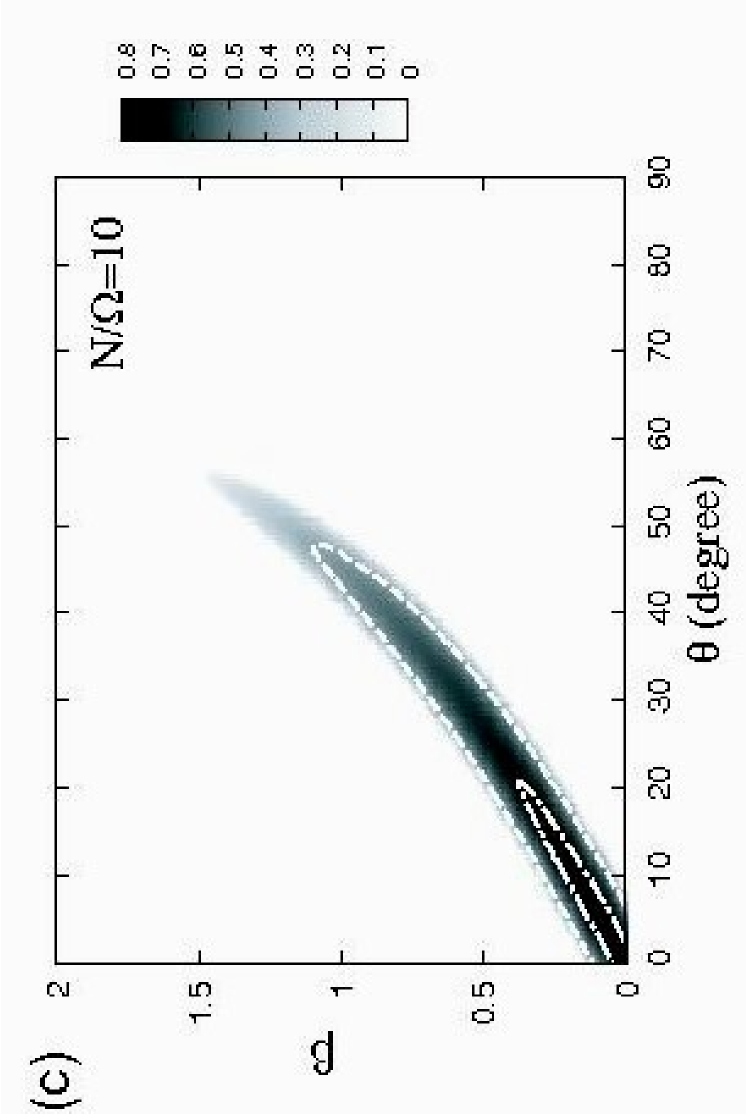
Figure 4: The contour plot of the growth rate of the NMRI modes ($m=29$) for the case of (a) $N/\Omega=0.1$, (b) $N/\Omega=1.0$, and (c) $N/\Omega=10$. The growth rate is shown on the $\theta$-$\beta$ diagram. The polar angle $\theta$ is defined as $\theta\equiv\tan^{-1}(r/z)$ and measured with a unit of degree. The contour lines in each figure denote $\gamma/\Omega=0.7$ (dot-dashed curve), 0.4 (dashed curve), and 0.2 (dotted curve). Model parameters are the same as those in Figure 1 except for the Brunt-Väisälä frequency $N$.

Figure 4 shows the effects of $N$ on the NMRI modes. The growth rate is shown by a gray contour on the $\theta$-$\beta$ plane for the case of $m=29$, which corresponds to the fastest growing mode of the NMRI. Since the size of the Brunt-Väisälä frequency in PNSs is highly uncertain (see § 5), we investigate a wide range of $N/\Omega$. From top to bottom, Figure 4 shows the results for $N/\Omega=0.1$, 1, and 10. The shear parameter is assumed to be $q=1.5$.

The growth rate of the NMRI decreases with increasing $N$. The stabilizing effect by the Brunt-Väisälä oscillation depends on the angle between the poloidal wavevector $k$ and $N$. When $N/\Omega=0.1$ (Fig. 4a), the effect of $N$ is weak, so that the growth rate is independent of $\theta$. The mode with $\beta=0$ is always the fastest and the maximum growth rate is $0.75\Omega$. When $N$ is comparable to $\Omega$ (Fig. 4b), the growth rate of the modes with $\mbox{\boldmath$k$}\perp\mbox{\boldmath$N$}$ is slightly suppressed due to the restoring force of $N$. On the other hand, unstable modes with the poloidal wavevector parallel to $N$ is unaffected by the Brunt-Väisälä oscillation and still have a growth rate of the order of the angular velocity $\Omega$. If the Brunt-Väisälä frequency is much larger than $\Omega$ (Fig. 4c), the unstable modes can exist only when $\mbox{\boldmath$k$}\parallel\mbox{\boldmath$N$}$. Near the equatorial plane ($\theta\gtrsim 60\arcdeg$), the growth of the NMRI ($m=29$) is completely suppressed.

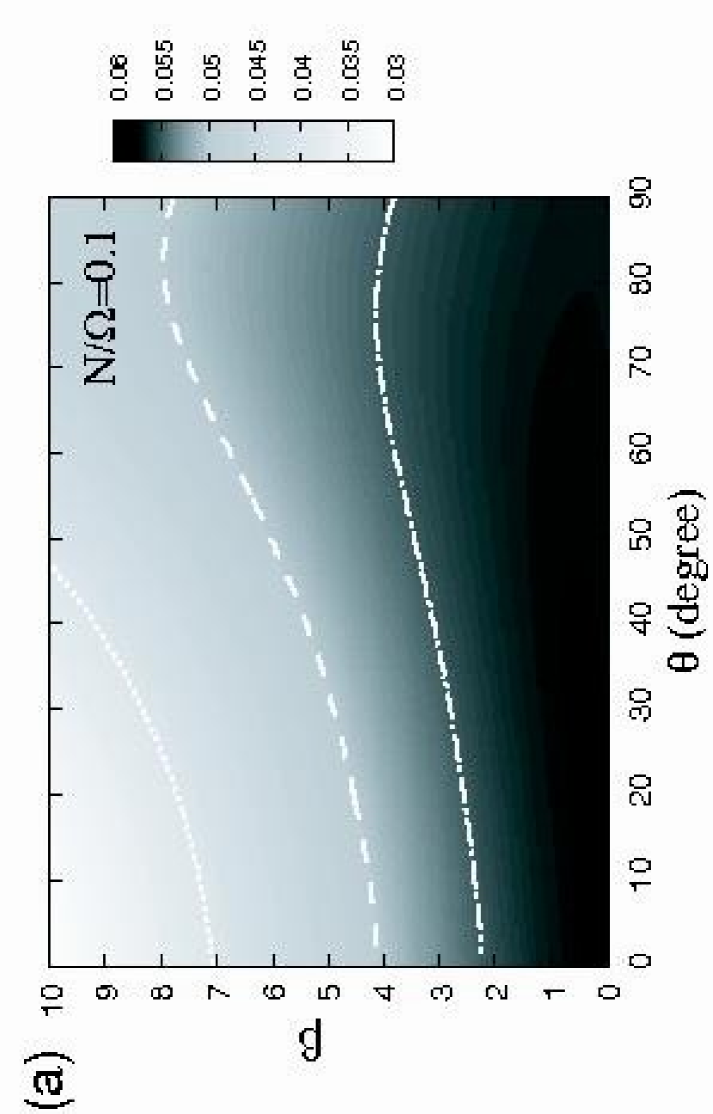
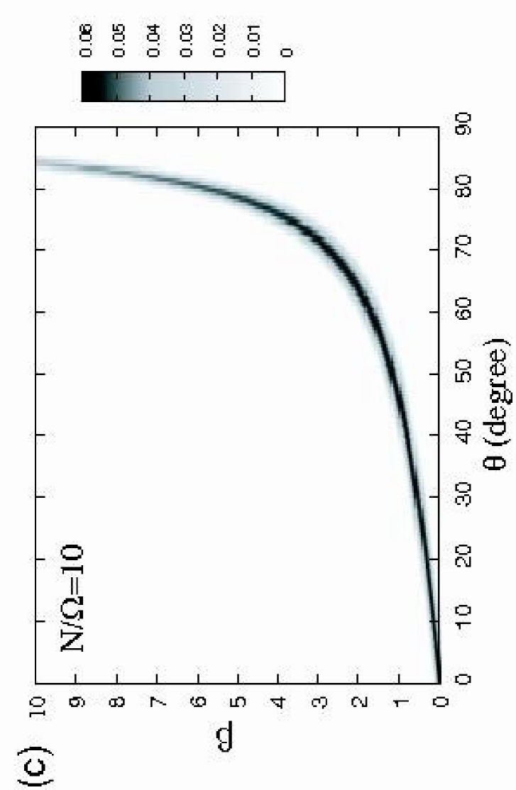
Figure 5: The contour plot of the growth rate of the kink modes ($m=1$) for the case of (a) $N/\Omega=0.1$, (b) $N/\Omega=1.0$, and (c) $N/\Omega=10$. The growth rate is shown on the $\theta$-$\beta$ diagram. The polar angle $\theta$ is defined as $\theta\equiv\tan^{-1}(r/z)$ and measured with a unit of degree. The contour lines in each figure denote $\gamma/\Omega=0.055$ (dot-dashed curve), 0.05 (dashed curve), and 0.04 (dotted curve). Model parameters are the same as those in Figure 1 except for the Brunt-Väisälä frequency $N$.

Next, we examine the effect of $N$ on the kink modes. Figure 5 shows the dimensionless growth rate $\gamma/\Omega$ as a function of $\beta$ and $\theta$ for the case of $m=1$. Notice that the growth rate of kink modes is much smaller than that of NMRI modes. When $N$ is comparable or larger than $\Omega$, almost all modes except that $k$ is parallel to $N$ are suppressed, the same as in the case of NMRI modes.

The difference between the NMRI and kink modes can be seen in the vicinity of the equatorial plane. The NMRI modes are suppressed around equatorial plane with increase of $N/\Omega$ (Fig. 4c). On the other hand, the kink modes can survive even near the equatorial plane (Fig. 5c). The direction of the entropy and leptonic gradients is almost horizontal when $\theta\sim 90\arcdeg$, so that only a mode with a wavevector $\mbox{\boldmath$k$}\parallel\mbox{\boldmath$N$}$, or $\beta=k_{r}/k_{z}\gg 1$, can grow against the Brunt-Väisälä oscillation. As seen in Figure 1, the kink mode can exist in the limit of $\beta\gg 1$, while the NMRI is suppressed completely. For the growth of the NMRI, the radial displacement of a perturbed fluid element is essential. However, the radial motion is stabilized near the equatorial plane and the NMRI cannot grow in such the situation. This would be the origin of the different behavior between two instabilities near the equatorial plane.

4 ANALYTICAL TREATMENT

In this section, we discuss the stability criteria and the maximum growth rate using an analytical approach. Since the dispersion equation (24) has a very complex form, it is difficult to treat for what it is. Therefore we simplify it under realistic approximations. Our simplified dispersion equation captures the features of the original equation precisely, so that our analytical stability criteria would be useful for applications to the stellar interiors.

The stability criteria for the cases of a weak differential rotation, $q\ll(\omega_{A}/\Omega)^{2}$, and a rigid rotation, $q=0$, have already been investigated in terms of the interior of normal stars (Fricke 1969; Tayler 1973; Acheson 1978; Schmitt & Rosner 1983; Pitts & Tayler 1986; Spruit 1999, 2002). Here we consider a strong differential rotation case, $q\gg(\omega_{A}/\Omega)^{2}$, because it would be common in PNSs. In that case, NMRI modes are dominant and then we can use the high rotational frequency approximation assuming that the growth rate is comparable to the angular velocity and much larger than the Alfvén frequency, $\omega\sim\Omega\gg\omega_{A}$.

4.1 Stability Criteria

The dispersion equation (24) can be rewrite as

$$\frac{k^{2}}{k_{z}^{2}}\left(\omega^{2}-m^{2}\omega^{2}_{A}\right)^{2}-\left[-2(1-s)\omega^{2}_{A}+\kappa^{2}+N^{2}_{e}\right]\left(\omega^{2}-m^{2}\omega^{2}_{A}\right)-4\omega^{2}_{A}\left(\omega+m\Omega\right)^{2}=0\;.$$ (30)

We consider a case of high rotational frequency, $\omega\sim\Omega\gg\omega_{A}$, and a large azimuthal wavenumber, $m\gg 1$. Then the Alfvén frequency in the second term can be negligible compared to the epicyclic and Brunt-Väisälä frequencies. We can also approximate $\omega+m\Omega\sim m\Omega$ in the third term. Using these approximations, we can obtain a simplified dispersion equation,

$$\frac{k^{2}}{k^{2}_{z}}\left(\omega^{2}-m^{2}\omega^{2}_{A}\right)^{2}-\left(\kappa^{2}+N^{2}_{e}\right)\left(\omega^{2}-m^{2}\omega^{2}_{A}\right)-4m^{2}\omega^{2}_{A}\Omega^{2}=0\;.$$ (31)

This is a quadratic equation of $\omega$ and the analytical solution is

$$\omega^{2}=m^{2}\omega^{2}_{A}+\frac{1}{2}\frac{k^{2}_{z}}{k^{2}}\left\{\kappa^{2}+N^{2}_{e}\pm\left[\left(\kappa^{2}+N^{2}_{e}\right)^{2}+16\frac{k^{2}}{k^{2}_{z}}m^{2}\omega^{2}_{A}\Omega^{2}\right]^{1/2}\right\}\;.$$ (32)

The stability condition is given by $\omega^{2}>0$, that is,

$$\left(\frac{k_{r}}{k_{z}}\right)^{2}A_{2}+\left(\frac{k_{r}}{k_{z}}\right)A_{1}+A_{0}>0\;,$$ (33)

where

$$A_{2}=m^{2}\omega^{2}_{A}+N^{2}_{z}\;,\ \ \ A_{1}=-2N_{r}N_{z}\;,\ \ \ A_{0}=N^{2}_{r}-2q\Omega^{2}+m^{2}\omega^{2}_{A}\;.$$ (34)

This inequality [eq. (33)] is satisfied if and only if (i) $A_{2}+A_{0}>0$ and (ii) $D=A^{2}_{1}-4A_{2}A_{0}<0$ . By using these two conditions, we can derive two criteria for stability;

$$\left(\frac{\omega_{A}}{\Omega}\right)^{2}m^{2}-q+\frac{1}{2}\left(\frac{N}{\Omega}\right)^{2}>0\;,$$ (35)

$$N^{2}\omega^{2}_{A}m^{2}-2q\Omega^{2}N^{2}_{z}>0\;.$$ (36)

These criteria are quadratic functions of the azimuthal wavenumber $m$. Thus, equations (35) and (36) are consistently satisfied for every azimuthal wavenumber in the case that zeroth order term of $m$ is positive. Therefore the general stability criteria can be derived as

$$N^{2}+{\frac{\partial\Omega^{2}}{\partial\ln r}}>0\;,$$ (37)

$$N^{2}_{z}\frac{\partial\Omega^{2}}{\partial\ln r}>0\;.$$ (38)

These criteria have forms similar to the Solberg-Høiland criteria but with gradients of angular velocity replacing the gradients of specific angular momentum. If the leptonic gradients are ignored, these criteria are exactly identical to those of the axisymmetric MRI (Balbus & Hawley 1995).

4.2 Maximum Growth Rate

The maximum growth rate of NMRI can be derived from equation (32). By differentiating partially with respect to $m$, the azimuthal wavenumber $m_{\rm{max}}$ that provides an extremum is obtained as

$$m_{\rm{max}}=\frac{1}{4\omega_{A}\Omega}\frac{k_{z}}{k}\left[16\Omega^{4}-\left(\kappa^{2}+N^{2}_{e}\right)^{2}\right]^{1/2}\;.$$ (39)

Substituting $m_{\rm{max}}$ into equation (32), the maximum growth rate with respect to $m$ is given by

$$\gamma_{\rm{max}}=\frac{q\Omega}{2}\frac{k_{z}}{k}\left(1-\frac{1}{2q}\frac{N^{2}_{e}}{\Omega^{2}}\right)\;.$$ (40)

We consider the characteristics of $\gamma_{\max}$ in two limiting cases, $N=0$ and $N\neq 0$. When $N=0$, the unstable growth rate takes the maximum value,

$$\gamma_{\rm{max}}=\frac{q\Omega}{2}\;,$$ (41)

when $k_{r}/k_{z}=0$ and

$$m_{\max}=\frac{\Omega}{2\omega_{A}}\sqrt{-q^{2}+4q}\;.$$ (42)

These results are consistent with the characteristics of the original dispersion equation (24) discussed in § 3.1.

If $N\neq 0$, the ratio of the poloidal wavenumbers for the fastest growing mode $\beta_{\rm{max}}$ can be obtained by differentiating equation (40) with respect to $\beta$. Then $\beta_{\rm{max}}$ should satisfy the following equation,

$$\left(\frac{N_{r}}{N_{z}}-\beta_{\max}\right)\left(\beta_{\max}^{2}+\frac{N_{r}}{N_{z}}\beta_{\max}+2\right)-2q\beta_{\max}\left(\frac{\Omega}{N_{z}}\right)^{2}=0\;.$$ (43)

When $N\gg\Omega$, we can solve this equation approximately and the solution is given by $\beta_{\rm{max}}\sim N_{r}/N_{z}$. This means that the poloidal wavevector of the fastest growing mode is parallel to the entropy and leptonic gradients ($\mbox{\boldmath$k$}\parallel\mbox{\boldmath$N$}$). This is also consistent with the results of the original dispersion equation shown in Figure 4.

5 APPLICATION TO PROTO-NEUTRON STARS

In this section, we apply the simplified dispersion equation (31) to the interiors of PNSs and investigate the stability for the NMRI. In order to do that, we must know the amplitude of the physical parameters in the dispersion equation. Here we estimate physical quantities of PNSs based on the observations of pulsars and the numerical simulations of core-collapse supernovae.

In the following we concentrate our discussions on the convectively stable regions in PNSs, which locates at the outer layer of PNSs (Janka & Müller 1996). If this region is magnetohydrodynamically unstable, neutrino luminosities would be amplified by various nonlinear magnetic processes (see § 6). The gain region behind the accretion shock is another site of MHD instabilities being important. Thompson et al. (2005) suggest that the viscous dissipation caused by MRI can enhance the heating in the gain region sufficiently enough to yield explosions. However, the gain region is convectively unstable. Convective motions may affect the growth of the MRI as is shown in convection-dominated accretion disks (Narayan et al. 2002). Although the linear and nonlinear interaction between the NMRI and convection would be a quite important issue, it is beyond the scope of this paper.

5.1 Physical Quantities in Proto-Neutron Stars

PNSs are expected to rotate differentially, as opposite to old neutron stars. Even when the iron core of a supernova progenitor is almost rigidly rotating (Heger et al. 2000; Heger et al. 2005), the collapse can generate a significant amount of differential rotation. Numerical studies of the rotating core-collapse indicate that the outer layers of PNSs would be rotating at the angular velocity $\Omega\simeq 100$ – $1000\ \rm{sec^{-1}}$ with a shear parameter $q\lesssim 1$ (Buras et al. 2003; Villain et al. 2004; Kotake et al. 2004). This angular velocity is comparable to the observations of young isolated pulsars associated with supernova remnants (Marshall et al. 1998). Thus, we adopt a rotational profile of $\Omega=100\ \rm{sec^{-1}}$ and $q\simeq 1$ as typical values in PNSs.

MHD simulations of the core-collapse suggest that toroidal magnetic fields would be much stronger than the poloidal component (Akiyama et al. 2003; Kotake et al. 2004; Yamada & Sawai 2004; Takiwaki et al. 2004; Ardeljan et al. 2005). This is because the toroidal component is generated by wrapping of poloidal fields by strong differential rotation during the core-collapse phase. On the other hand, observations of young isolated pulsars indicate that poloidal magnetic fields of neutron stars are typically of the order of $10^{12-13}$ G. Thus we expect that the toroidal fields at the interiors of PNSs could be $10^{13}$ G. When we employ $B_{\phi}=10^{13}$ G, the Alfvén frequency is

$$\omega_{A}\simeq 3.0\left(\frac{B_{\phi}}{10^{13}\ \rm{G}}\right)\left(\frac{r}{10^{6.5}\ \rm{cm}}\right)^{-1}\left(\frac{\rho}{10^{11}\ \rm{g}\ \rm{cm}^{-3}}\right)^{-1/2}\ \rm{sec^{-1}}\;.$$ (44)

The size of the Brunt-Väisälä oscillation in the stably stratified layer of PNSs is sensitive to microscopic physics such as the equation of state and neutrino opacity (Buras et al. 2003; Kotake et al. 2004; Thompson et al. 2005; Dessart et al. 2005). Therefore, we treat the Brunt-Väisälä frequency as a parameter. Because the Brunt-Väisälä frequency would be larger than the Alfvén frequency in the stellar interiors, $N^{2}\gg\omega^{2}_{A}$, the models with $N/\Omega=0.1$ – $10$ are examined here. We use our simplified dispersion equation (31) for the stability analysis. This equation does not include the parameter $s$, so that we can neglect the effects of field distribution in the following discussion.

5.2 Stability of Proto-Neutron Stars

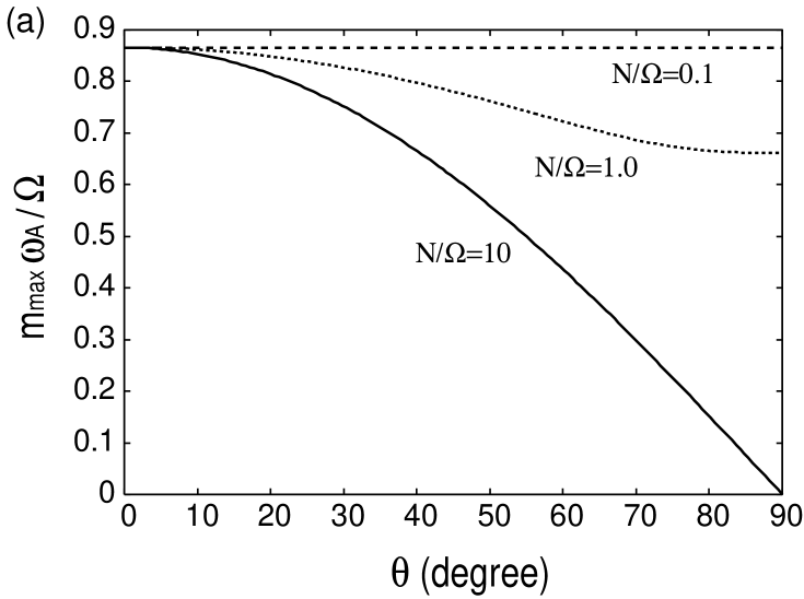
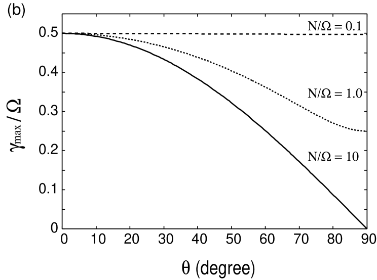
Figure 6: (a) The azimuthal wavenumber and (b) the maximum growth rate of the fastest growing mode as a function of the polar angle $\theta$ for the cases with $N/\Omega=0.1$, 1.0, and 10. These are obtained from our simplified dispersion equation (31). We choose the model parameters as $q=1.0$, $\Omega=100\ \rm{sec^{-1}}$, and $\omega_{A}=3\ \rm{\sec^{-1}}$.

The characteristics of the NMRI in stably stratified layers of PNSs are shown in Figure 6. We assume the physical parameters $q=1$, $\Omega=100\ \rm{sec^{-1}}$, and $\omega_{A}=3.0\ \rm{sec^{-1}}$. For the Brunt-Väisälä frequency, we examine three cases with $N/\Omega=0.1$, 1, and 10.

Figure 6a depicts the normalized azimuthal wavenumber of the fastest growing mode $m_{\rm{max}}\omega_{A}/\Omega$ obtained from equations (39) and (43). The characteristic wavenumber $m_{\max}$ depends on the polar angle $\theta$ and the Brunt-Väisälä frequency $N$. Figure 6b shows the dimensionless maximum growth rate $\gamma_{\rm{max}}/\Omega$ as a function of the polar angle $\theta$. The maximum growth rate $\gamma_{\rm{max}}$ is determined by $\beta_{\rm{max}}$ using equation (40). When the Brunt-Väisälä frequency is small $N/\Omega=0.1$, the azimuthal wavenumber $m_{\rm{max}}$ is independent of the polar angle $\theta$. The maximum growth rate $\gamma_{\rm{max}}$ is constant at a value given by equation (41), which means that the NMRI is quite important in the entire regions. If the Brunt-Väisälä frequency $N$ is comparable to the angular velocity $N/\Omega=1$, the maximum growth rate decreases near the equatorial plane. However the decrease of the growth rate is at most by a factor of 2 at $\theta\sim 90\arcdeg$. The azimuthal wavenumber is much larger than unity at any angle $\theta$ so that the NMRI is still dominant over the kink-type instability.

Even when $N/\Omega$ is much larger than unity, all the regions are magnetohydrodynamically unstable. However the kink modes are dominant in the vicinity of the equator and thus the maximum growth rate decreases by many orders. Near the rotational axis, on the other hand, the azimuthal wavenumber $m_{\max}$ and the maximum growth rate $\gamma_{\rm{max}}$ are unaffected by the Brunt-Väisälä frequency $N$. We define the critical angle $\theta_{\rm crit}$ at where the maximum growth rate becomes half of the value at $\theta=0$. The critical angle is about $\theta\sim 60\arcdeg$ for the case of $N/\Omega=10$. We find that the critical angle is independent of the Brunt-Väisälä frequency if $N/\Omega\gtrsim 10$.

As a result, we can conclude that stably stratified layers of PNSs are always unstable to MHD instabilities. For the cases of $N/\Omega<1$, the NMRI can grow at any angle $\theta$. Even when $N/\Omega$ is larger than unity, the polar regions is unstable to the NMRI. The growth rate is comparable to the angular velocity $\Omega$ and much faster than that of the kink modes. The kink modes can be dominant only in the vicinity of the equator when the Brunt-Väisälä frequency exceeds the angular velocity. The typical growth time of NMRI is about 100 msec. This is much shorter than the neutrino cooling time of PNSs ($\sim 10$ sec), and thus the nonlinear growth of NMRI may affect the neutrino luminosities.

We adopt $\Omega/\omega_{A}=30$ as a typical value in the discussions above. Recent numerical studies of rotating core-collapse suggests the possibility of more rapidly rotating PNSs up to $\Omega\simeq 1000$ sec^-1 (Fryer & Heger 2000; Dimmelmeier et al. 2002; Thompson et al. 2005) and more strongly magnetized PNSs with $B_{\phi}\simeq 10^{15}$ G as an origin of magneters (Kotake et al. 2004; Yamada & Sawai 2004; Takiwaki et al. 2005; Sawai et al. 2005). Therefore, it would be interesting to consider the rapidly rotating case, $\Omega/\omega_{A}\gtrsim 100$, and strongly magnetized case, $\Omega/\omega_{A}\simeq 1$.

The growth rate of the NMRI is proportional to the angular velocity. For rapidly rotating PNSs ($\Omega/\omega_{A}\gtrsim 100$), the NMRI can grow in shorter time scale than 10 msec. The characteristic length scale in the azimuthal direction, $v_{\rm A}/\Omega$, shifts to the shorter wavelength. In strongly magnetized PNSs ($\Omega/\omega_{A}\simeq 1$), on the other hand, the NMRI is stabilized by the strong magnetic tension. The critical azimuthal wavenumber for the growth of NMRI is given by $\sqrt{2q}\ \Omega/\omega_{A}$, and thus the NMRI modes would be suppressed completely if the field is very strong $\omega_{\rm A}\sim\Omega$. Only the kink modes can survive in such a situation because they are not affected by the magnetic tensions.

6 DISCUSSION

6.1 Effects of Diffusion Processes

In the interior of PNSs, neutrino radiation plays an important role in the heat and lepton transports. The thermal and lepton diffusions caused by the neutrino radiation can reduce both the thermal and leptonic buoyant frequencies significantly. The coefficients of the thermal and chemical diffusivities in PNSs are given by

$$\kappa_{\rm{T}}\simeq 10^{9}\ Y^{-1}_{1/3}l^{2}_{30}\frac{T_{4}}{\mu^{6}_{20}}\ {\rm cm}^{2}\ \sec^{-1}\;,\ \ \ \nu_{\rm{chem}}\simeq 10^{9}\ l^{2}_{30}\frac{T_{4}}{\mu^{6}_{20}}\ \ {\rm cm}^{2}\ \sec^{-1}\;,$$ (45)

where $Y_{1/3}$ is the electron fraction in units of $1/3$, $l_{30}$ is a length scale in units of 30 km, $T_{4}$ is the temperature in units of 4 MeV, and $\mu_{20}$ is the electron chemical potential normalized by 20 MeV (Socrates et al. 2005).

These diffusion processes must be considered if the wavelength of fluctuations is shorter than the critical length scale that can be estimated by equating the diffusion time and the period of the buoyant oscillations. The critical length scale of the thermal diffusion is given by $\lambda_{\rm{T}}\sim\sqrt{\kappa_{\rm{T}}/N_{\rm{T}}}\simeq 10^{3}$ cm, where we assume $N_{T}\simeq 1000$ sec^-1. The critical length of the chemical diffusion may be a few times larger than that of the thermal one, because the leptonic buoyant frequency is smaller than $N_{\rm T}$ (Thompson & Murray 2000). Thus, our analysis is valid for the wavelength of the perturbations longer than the diffusion length $\lambda_{\rm T}$.

However, the diffusive processes could affect the growth of the NMRI for the shorter wavelength $\lambda<\lambda_{\rm{T}}$. The primary effect of the thermal and chemical diffusions is to reduce the restoring force caused by the stable stratification (Acheson 1978; Spruit 1999). Therefore, the maximum growth rate of NMRI increases and approaches to the case of $N/\Omega\rightarrow 0$ when $\lambda\ll\lambda_{\rm T}$. Thus, the growth of these shorter wavelength modes may be dominant in the stably stratified layers of PNSs.

6.2 NMRI Modes vs. Kink Modes

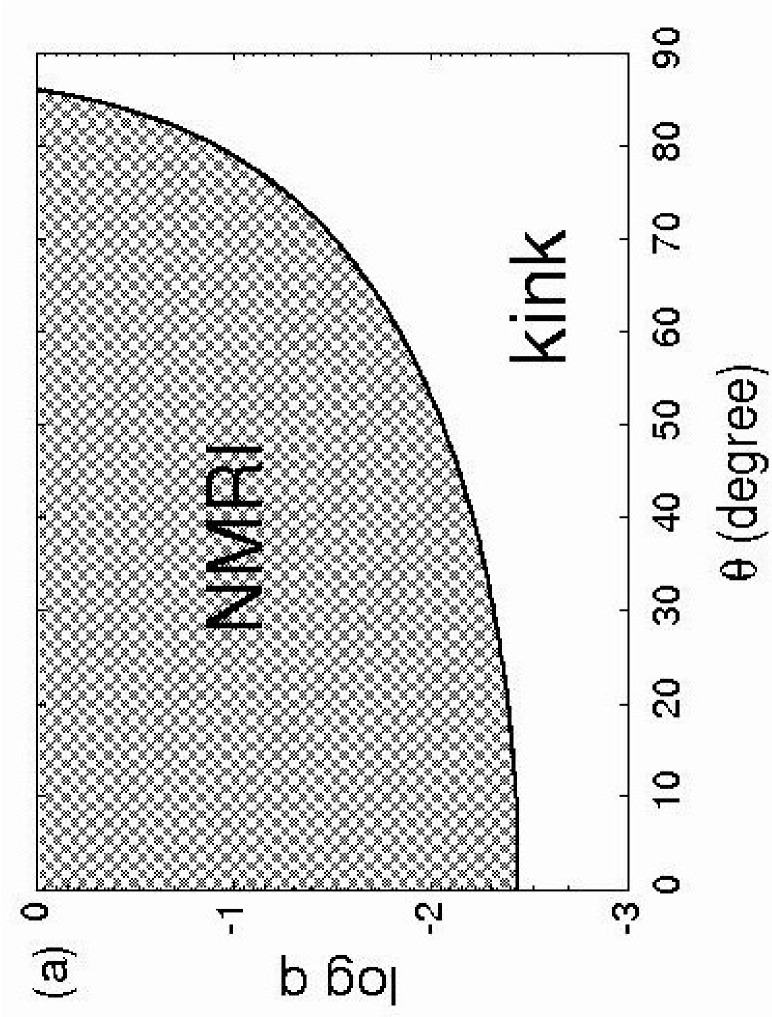
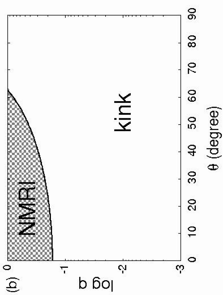
Figure 7: (a) The NMRI and kink dominant regimes in the diagram of the shear parameter $q$ and the polar angle $\theta$ for the case of the PNSs. The border of the two regions is where the maximum azimuthal wavenumber is $m_{\max}=2$ in equation (39). Model parameters for this case are $N=10\Omega$ and $\Omega=30\omega_{A}$. (b) The same plot for the case of the solar radiative zone. Model parameters are $N=10^{3}\Omega$ and $\Omega=5\omega_{A}$.

The conditions that the NMRI modes dominate over the kink modes can be derived from our simplified dispersion equation (31). The NMRI modes grow faster if the azimuthal wavenumber $m_{\max}$ is more than 2. The shaded (white) area in Figure 7a represents the NMRI (kink) dominant region in the $q$-$\theta$ diagram. The boundary of these two areas is given by where $m_{\rm{max}}=2$ is fulfilled in equation (39). In this figure, we assume $N/\Omega=10$ and $\Omega/\omega_{A}=30$ which are the typical values in PNSs. The NMRI modes are dominant at most of the regions if the shear parameter $q$ is relatively large ($q\gtrsim 10^{-2}$). The kink modes become important only when the shear parameter is extremely smaller than unity. The boundary curve is little changed by the size of the Brunt-Väisälä frequency.

For comparison, a similar picture for the solar radiative zone is shown by Figure 7b. In the solar radiative zone, the Brunt-Väisälä frequency is much larger than the angular velocity $N/\Omega\simeq 10^{3}$ (Spruit 2002). Here we assume the Alfvén frequency $\Omega/\omega_{A}=5$ as the typical value in the solar radiative zone. The parameter region where the kink modes are dominant extends to the larger $q$ regime because of the smaller ratio of $\Omega/\omega_{A}$. Only when the shear rate is about unity, the NMRI modes can be important for this case. According to the helioseismology, the solar radiative zone exhibits a nearly rigid rotation ($q\ll 1$). Thus, the kink modes are dominant and Tayler-Spruit dynamo would be amplifying the magnetic fields (Spruit 2002).

6.3 Nonlinear Growth of the NMRI

The NMRI can grow in the stably stratified layer of PNSs regardless of the size of the Brunt-Väisälä frequency. The nonlinear growth of the NMRI could initiate and sustain MHD turbulence and amplify magnetic fields. As is well known in the contexts of accretion disks, MHD turbulence leads to the angular momentum transport. Thus the rotational configurations within PNSs evolve toward a rigid rotation. If the PNSs will rotate rigidly, the neutrino sphere become oblate and the neutrino luminosies could be enhanced in the polar region (Kotake et al. 2003). Thus, the polar region would be heated by neutrinos preferentially.

Turbulent viscosity generated by the NMRI can convert the rotational energies into the thermal energies, so that the neutrino luminosities from the PNSs may be increased (Thompson et al. 2005). Ramirez-Ruiz & Socrates (2005) suggest that the heating of materials through magnetic reconnection may also lead to the enhancement of neutrino luminosity. We would like to stress that the magnetoconvection and magnetic Rayleigh-Taylor instability of magnetic flux tube would assist the mixing of materials in the layers where is heretofore thought to be convectively stable (Parker 1974, 1975, 1979).

Although these effects are absolutely a matter of speculation, it is sure that these effects are not considered in the present scenarios of core-collapse supernovae. Therefore, we anticipate that these multiple magnetic effects can enhance the neutrino luminosity sufficiently to yield explosions in models that would otherwise fail. Because these magnetic phenomena are essentially three-dimensional, we must perform three-dimensional MHD simulations to reveal those effects quantitatively. This is our future work.

7 SUMMARY

In this paper, we perform the local linear analysis of the stably stratified layers in stellar objects taking account of toroidal magnetic fields and differential rotation. We derive the local dispersion equation and apply it to the interior of PNSs. Our findings are summarized as follows.

1. NMRI modes are dominant when the rate of differential rotation $q$ is large and the growth rate is comparable to the angular velocity. In the limit of rigid rotation ($q\to 0$), only $m=1$ mode is unstable, which corresponds to the kink instability. The growth rate of the kink mode is given by $\omega^{2}_{A}/\Omega$ and typically much smaller than that of the NMRI.

2. The growth of NMRI is suppressed by the Brunt-Väisälä oscillation. However, because the stabilizing force is along the direction of the entropy and leptonic gradients $N$, the unstable modes can exist if the wavevector is parallel to $N$. Thus the kink modes is dominant over the NMRI modes in the vicinity of the equator when $N/\Omega$ is large.

3. Analytical formula of the stability criteria for NMRI and the maximum growth rate are derived from our simplified dispersion equation. The stability criteria are completely identical to those for the axisymmetric MRI if the leptonic gradient is ignored. The maximum growth is also agreed with that of the axisymmetric MRI for the case of $N=0$.

4. NMRI can grow in the interiors of differentially rotating PNSs in spite of the size of the Brunt-Väisälä frequency. The suppression by the Brunt-Väisälä oscillation can be seen only near the equatorial plane where the kink mode is dominating. The typical growth time of NMRI is about 100 m sec, which is much shorter than the neutrino cooling time of PNSs.

References

- Acheson (1978) Acheson, D. J. 1978, Phil. Trans. Roy. Soc. Lond. A 289, 459
- Akiyama et al. (2003) Akiyama, S., Wheeler, J. C., Meier, D. L., & Lichtenstadt, I. 2003, ApJ, 584, 954
- Ardeljan (2005) Ardeljan, N. V., Bisnovatyi-Kogan, G. S., Moiseenko, S. G. 2005, MNRAS, 359, 333
- Arnett (1987) Arnett, W. D. 1987, ApJ, 319, 136
- Balbus & Hawley (1991) Balbus, S. A., & Hawley, J. F. 1991, ApJ, 376, 214
- Balbus & Hawley (1992) Balbus, S. A., & Hawley, J. F. 1992, ApJ, 400, 610
- Balbus & Hawley (1994) Balbus, S. A., & Hawley, J. F. 1994, MNRAS, 266, 769
- Balbus & Hawley (1995) Balbus, S. A., & Hawley, J. F. 1995, ApJ, 453, 380
- Balbus & Hawley (1998) Balbus, S. A., & Hawley, J. F. 1998, Rev. Mod. Phys, 70, 1
- Bethe (1990) Bethe, H. 1990, Rev. Mod. Phys, 62, 801
- Bruenn & Dineva (1996) Bruenn, S. W., & Dineva, T. 1996, ApJ, 458, L71
- Bruenn et al (2004) Bruenn, S. W., Raley, E. A., & Mezzacappa, A. 2004, preprint (astro-ph/0404099)
- Buras et al. (2003) Buras, R., Rampp, M., Janka, H.-T., & Kifonidis, K. 2003, Phys. Rev. Lett., 90, 241101
- Burrows & Lattimer (1986) Burrows, A., & Lattimer, J. 1986, ApJ, 307, 178
- Burrows & Fryxell (1993) Burrows, A., & Fryxell, B. 1993, ApJ, 418, L33
- Burrows et al (1993) Burrows, A., Hayes, J., & Fryxell, B. 1993, ApJ, 450, 830
- Chandrasekhar (1961) Chandrasekhar, S., 1961 Hydrodynamic and Hydromagnetic Stability (Oxford University Press)
- Dessart et al. (2005) Dessart, L., Burrows, A., Livne, E., & Ott, C.D. 2005, preprint (astro-ph/0510229)
- Dimmelmeier et al. (2002) Dimmelmeier, H., Font, J. A, & Müller, E. 2002, A&A, 393, 523
- Epstein (1979) Epstein, R. 1979, MNRAS, 188, 305
- Fricke (1969) Fricke, K. 1969, A&A, 1, 338
- Fryer & Heger (2000) Fryer, C. L., & Heger, A. 2000, ApJ, 541, 1033
- Goldreich & Lynden-Bell (1965) Goldreich, P., & Lynden-Bell, D. 1965, MNRAS, 130, 125
- Heger et al. (2000) Heger, A., Langer, N., & Woosley, S. E. 2000, ApJ, 528, 368
- Heger et al. (2005) Heger, A., Woosley, S. E., Langer, N., & Spruit, H. C. 2005, ApJ, 626, 350
- Janka & Müller (1996) Janka, H.-T., & Müller, E. 1996, A&A, 306, 167
- Keil et al. (1996) Keil, W., Janka, H.-T., & Müller, E. 1996, ApJ, 473, L111
- Kim & Ostriker (2000) Kim, W.-T., & Ostriker, E. C. 2000, ApJ, 540, 372
- Kotake et al. (2003) Kotake, K., Yamada, S., & Sato, K. 2003, ApJ, 595, 304
- Kotake et al. (2004) Kotake, K., Sawai, H., Yamada, S., & Sato, K. 2004, ApJ, 608, 391
- Lattimer & Mazurek (1981) Lattimer, J. M., & Mazurek, T. J. 1981, ApJ, 246, 955
- LeBlanc & Wilson (1970) LeBlanc, J. M., & Wilson, J. R. 1970, ApJ, 161, 541
- Marshall et al. (1998) Marshall, F. E., Gotthelf, E. V., Zhang, J.-P., Middleditch, J., & Wang, Q. D. 1998, ApJ, 499, L179
- Mayle. (1985) Mayle, R. W., 1985, Ph.D thesis, Univ. California, Barkeley
- Mezzacappa et al. (1998) Mezzacappa, A., Calder, A. C., Bruenn, S. W., Blondin, J. M., Guidry, M. W., Strayer, M. R., & Umar, A. S. 1998a, ApJ, 493, 848
- Mezzacappa et al. (1998) Mezzacappa, A., Calder, A. C., Bruenn, S. W., Blondin, J. M., Guidry, M. W., Strayer, M. R., & Umar, A. S. 1998b, ApJ, 495, 911
- Miralles et al. (2000) Miralles, J. A., Pons, J. A., & Urpin, V. 2000, ApJ, 543, 1001
- Miralles et al. (2002) Miralles, J. A., Pons, J. A., & Urpin, V. 2002, ApJ, 574, 356
- Miralles et al. (2004) Miralles, J. A., Pons, J. A., & Urpin, V. 2004, A&A, 420, 245
- Narayan et al. (2002) Narayan, R., Quataert, E., Igumenshchev, I. V., & Abramowicz, M. A. 2002, ApJ, 577, 295
- Parker (1974) Parker, E.N. 1974, Ap&SS, 31, 261
- Parker (1975) Parker, E.N. 1975, ApJ, 198, 205
- Parker (1979) Parker, E.N. 1979, Ap&SS, 62, 135
- Pitts & Tayler (1985) Pitts, E., & Tayler, R. J. 1985, MNRAS, 216, 139
- Ramirez-Ruiz & Socrates (2005) Ramirez-Ruiz, E., & Socrates, A. 2005, preprint (astro-ph/0504257)
- Sawai et al. (2005) Sawai, H., Kotake, K., & Yamada, S. 2005, ApJ, 631, 446
- Schmitt & Rosner (1983) Schmitt, J. H. M. M., & Rosner, R. 1983, ApJ, 265, 901
- Socrates et al. (2005) Socrates, A., Blaes, O., Hungerford, A., & Fryer, C. L. 2005, ApJ, 632, 531
- Spruit (1999) Spruit, H. C. 1999, A&A, 349, 189
- Spruit (2002) Spruit, H. C. 2002, A&A, 381, 923
- Takiwaki et al. (2004) Takiwaki, T., Kotake, K., Nagataki, S., & Sato, K. 2004, ApJ, 616, 1086
- Tayler (1973) Tayler, R. J. 1973, MNRAS, 161, 365
- Terquem & Papaloizou (1996) Terquem, C., & Papaloizou, J. C. B. 1996, MNRAS, 279, 767
- Thompson & Murray. (2000) Thompson, C., & Murray, N. 2000, ApJ, 560, 339
- Thompson et al. (2005) Thompson, T. A., Quataert, E., & Burrows, A. 2005, ApJ, 620, 861
- Villain et al. (2004) Villain, L., Pons, J. A., Cerdá-Durán, P., & Gourgoulhon, E. 2004, A&A, 418, 283
- Wilson & Mayle (1988) Wilson, J.R., & Mayle, R.W. 1988, Phys. Rep., 163, 63
- Wilson & Mayle (1993) Wilson, J.R., & Mayle, R.W. 1993, Phys. Rep., 227, 97
- Yamada & Sawai (2004) Yamada, S., & Sawai, H. 2004, ApJ, 608, 907