Approximate dynamics of dark matter ellipsoids

Abstract

The collapse of a non-collisional dark matter and the formation of pancake structures in the universe are investigated approximately. Collapse is described by a system of ordinary differential equations, in the model of a uniformly rotating, three-axis, uniform density ellipsoid. Violent relaxation, mass, and angular momentum losses are taken into account phenomenologically. The formation of the equilibrium configuration, secular instability and the transition from a spheroid to a three-axis ellipsoid are investigated numerically and analytically in this dynamical model.

1 Introduction

According to modern cosmological ideas, most of the matter in the Universe is in the form of so-called cold dark matter, consisting of non-relativistic particles. The study of the formation of dark matter objects in the Universe is based on N-body simulations, which are very time consuming. In this situation, a simplified approach may become useful, because it allows one to investigate many different variants and to obtain some new principally important features of the problem, which could be lost or not visible during long numerical work.

The systematic analysis of ellipsoidal figures of equilibrium is presented in the classical book of Chandrasekhar (1969). Different types of incompressible ellipsoids are investigated there on the basis of virial equations, as well as their dynamical and secular stability. In particular, the points of onset of the bar-mode dynamical and secular instabilities of the Maclaurin spheroid, for its transition to the Jacobi ellipsoid, are found. Lynden-Bell (1964, 1965) applied the Chandrasechar’s virial tensor method for a rotating, self-gravitating spheroid of pressure-free gas and showed the growth of non-axisymmetric perturbations during collapse. It was also discussed that the slowly shrinking Maclaurin spheroid will enter the Jacobi series if it shrinks slowly enough for the dissipative mechanisms to be operative. There have been numerical investigations of collapsing pressureless spheroids in the papers of Lynden-Bell (1964) and Lin, Mestel & Shu (1965). The dynamics of a non-rotating sphere in two dimensions was considered in Lynden-Bell (1979), and it was shown that the pressure prevents the development of large-scale shape instability if initially the gravity is more than three-fifths pressure resisted. There is a wide-ranging review of this topic in the paper of Lynden-Bell (1996) in memory of Chandrasekhar.

Subsequent investigations of rapidly rotating figures are connected with stars, and with large-scale structure of the Universe. In Rosensteel & Huy (1991) the virial equations for rotating Riemann ellipsoids of incompressible fluid are demonstrated to form a Hamiltonian dynamical system. There is a detailed description of the ellipsoid model of rotating stars in the papers of Lai, Rasio & Shapiro (1993); Lai, Rasio & Shapiro (1994a); Lai, Rasio & Shapiro (1994b). Using a variational principle, they derived and investigated the equations for the evolution of a compressible Riemann-S ellipsoid, incorporating viscous dissipation and gravitational radiation. The solutions of these approximate equations permitted them to obtain equilibrium models, and to investigate their dynamical and secular stability. In a recent paper (Shapiro, 2004) secular bar-mode instability driven by viscous dissipation was investigated, using these equations, and the point of instability of compressible Maclaurin spheroids was found.

The modern theory of a large-scale structure is based on the ideas of Zel’dovich (1970), concerning the formation of strongly non-spherical structures during non-linear stages of the development of gravitational instability, known as ‘Zel’dovich’s pancakes’. Numerical simulations for these objects have been performed subsequently by many groups. In the case of structures in dark matter, we are dealing with non-collisional non-relativistic particles, interacting only by gravitation. The development of gravitational instability and collapse in dark matter do not lead to any shock formation or radiation losses, but are characterized by non-collisional relaxation. This relaxation is based on the idea of a ‘violent relaxation’ of Lynden-Bell (1967).

Here we derive and solve the equations for the dynamical behaviour in a simple model of a compressible uniformly rotating ellipsoid. We derive the equations for axes with the help of variation of the Lagrange function of an ellipsoid. Correct description of pressure effects, attained by such an approach, and the addition of relaxation permit us to obtain the dynamics of motion without any numerical singularities. In our model, motion along three axes takes place in the gravitational field of a uniform density ellipsoid, with account of the isotropic pressure, represented in an approximate non-differential way. Relaxation leads to a transformation of the kinetic energy of ordered motion into kinetic energy of chaotic motion, and to increases in the effective pressure and thermal energy. All losses are connected with runaway particles. The collapse of the rotating three-axis ellipsoid is approximated by a system of ordinary differential equations, where relaxation and losses of energy, mass and angular momentum are taken into account phenomenologically. The system is solved numerically for several parameters, characterizing the configuration. The approach in this work is similar to that used in Bisnovatyi-Kogan (2004), where only dark matter spheroids ($a=b\neq c$) were considered. In this case there are analytical formulae for the gravitational potential and forces. In the description of violent relaxation and different kinds of losses, we use the same approach as Bisnovatyi-Kogan (2004). In the present paper we also find the point of the onset of secular instability of a compressible Maclaurin spheroid, using the derived dynamical equations, and also from the analysis of the sequence of equilibrium configurations. A simple analytical formula for the point of onset of the bar-mode secular instability of the Maclaurin spheroid is found.

2 Equations of motion

Let us consider a three-axis ellipsoid, consisting of non-collisional, non-relativistic particles, with semi-axes $a\neq b\neq c$

$$\frac{x^{2}}{a^{2}}+\frac{y^{2}}{b^{2}}+\frac{z^{2}}{c^{2}}=1,$$ (1)

and rotating uniformly with angular velocity $\Omega$ around the $z$-axis. Let us approximate the density of the matter, $\rho$, in the ellipsoid as uniform.

The mass $m$ and total angular momentum $M$ of the uniform ellipsoid are connected with uniform density, angular velocity and semi-axes as ($V$ is the volume of the ellipsoid)

$$m=\rho\,V=\frac{4\pi}{3}\,\rho\,abc\,,\quad M=\rho\,\Omega\int\limits_{V}(x^{2}+y^{2})\,dV=\frac{m}{5}\,\Omega(a^{2}+b^{2})\,.$$ (2)

We assume a linear dependence of the velocities on the coordinates in the rotating frame,

$$\upsilon_{x}=\frac{\dot{a}x}{a}\>,\quad\upsilon_{y}=\frac{\dot{b}y}{b}\>,\quad\upsilon_{z}=\frac{\dot{c}z}{c}\,.$$ (3)

The gravitational energy of the uniform ellipsoid is defined as (Landau & Lifshitz, 1993)

$$U_{g}=-\frac{3Gm^{2}}{10}\int\limits_{0}^{\infty}\frac{du}{\sqrt{(a^{2}+u)(b^{2}+u)(c^{2}+u)}},$$ (4)

and is expressed in elliptical integrals (Gradshtein & Ryzhik, 1962). Let us consider a compressible ellipsoid with a constant mass and angular momentum, a total thermal energy of non-relativistic dark matter particles $E_{th}\sim V^{-2/3}\sim(abc)^{-2/3}$ and the relation between pressure $P$ and thermal energy $E_{th}$ as $E_{th}=\frac{3}{2}PV$. In absence of any dissipation, this ellipsoid is a conservative system. To derive the equations of motion, let us write the Lagrange function of the ellipsoid:

$$L=U_{kin}-U_{pot}\,,\quad U_{pot}=U_{g}+E_{th}+U_{rot}\>,$$ (5)

$$U_{kin}=\frac{1}{2}\,\rho\int\limits_{V}(\upsilon_{x}^{2}+\upsilon_{y}^{2}+\upsilon_{z}^{2})\,dV=\frac{m}{10}\,(\dot{a}^{2}+\dot{b}^{2}+\dot{c}^{2})\>,\quad E_{th}=\frac{E_{th,in}(a_{in}b_{in}c_{in})^{2/3}}{(abc)^{2/3}}=\frac{\varepsilon}{(abc)^{2/3}}\>,$$ (6)

where the entropy function $\varepsilon$ is constant in the conservative case, but variable in the presence of dissipation, and

$$U_{rot}=\frac{1}{2}\,\rho\int\limits_{V}V_{rot}^{2}\,dV=\frac{1}{2}\,\rho\,\Omega^{2}\int\limits_{V}(x^{2}+y^{2})\,dx\,dy\,dz=\frac{m}{10}\,\Omega^{2}(a^{2}+b^{2})\>.$$ (7)

Taking into account the second expression in (2), we obtain the relation

$$U_{rot}=\frac{5}{2}\,\frac{M^{2}}{m(a^{2}+b^{2})}\>.$$ (8)

By variation of the Lagrange function we obtain Lagrange equations of motion:

$$\ddot{a}=-\frac{3Gm}{2}\,a\int\limits_{0}^{\infty}\frac{du}{(a^{2}+u)\Delta}\,\,+\,\frac{10}{3m}\,\frac{1}{a}\,\frac{\varepsilon}{(abc)^{2/3}}\,\,+\frac{25M^{2}}{m^{2}}\,\frac{a}{(a^{2}+b^{2})^{2}}\,,$$ (9)

$$\ddot{b}=-\frac{3Gm}{2}\,b\int\limits_{0}^{\infty}\frac{du}{(b^{2}+u)\Delta}\,\,+\,\frac{10}{3m}\,\frac{1}{b}\,\frac{\varepsilon}{(abc)^{2/3}}\,\,+\frac{25M^{2}}{m^{2}}\,\frac{b}{(a^{2}+b^{2})^{2}}\,,$$ (10)

$$\ddot{c}=-\frac{3Gm}{2}\,c\int\limits_{0}^{\infty}\frac{du}{(c^{2}+u)\Delta}\,\,+\,\frac{10}{3m}\,\frac{1}{c}\,\frac{\varepsilon}{(abc)^{2/3}}\;,\;\;\Delta^{2}=(a^{2}+u)(b^{2}+u)(c^{2}+u)\,.$$ (11)

It is easy to check that the equilibrium solution of these equations are the Maclaurin spheroid and the Jacobi ellipsoid (Chandrasekhar, 1969).

3 Equations of motion with dissipation

In reality there is relaxation in the collisionless system, connected with phase mixing, which is called ‘violent relaxation’ (Lynden-Bell, 1967). This relaxation leads to a transformation of the kinetic energy of ordered motion into kinetic energy of chaotic motion and increases the effective pressure and thermal energy.

The main transport process is an effective bulk viscosity. Therefore, there is a drag force, which is described phenomenologically by adding the terms

$$-\frac{\dot{a}}{\tau_{rel}}\>,\quad-\frac{\dot{b}}{\tau_{rel}}\>,\quad-\frac{\dot{c}}{\tau_{rel}}$$ (12)

on the right-hand sides of the equations of motions.

Here we have scaled the relaxation time $\tau_{rel}$ by the Jeans characteristic time

$$\tau_{J}=\frac{2\pi}{\omega_{J}}=\frac{2\pi}{\sqrt{4\pi Gm}}=2\pi\sqrt{\frac{abc}{3Gm}}$$ (13)

with a constant value of $\alpha_{rel}$,

$$\tau_{rel}=2\pi\,\alpha_{rel}\sqrt{\frac{abc}{3Gm}}\,.$$ (14)

The process of relaxation is also accompanied by total energy $U_{tot}$, mass and angular momentum losses from the system. These losses may be described phenomenologically by characteristic times $\tau_{el}$, $\tau_{ml}$ and $\tau_{Ml}$, scaled by $\tau_{J}$ with the coefficients $\alpha_{el}$, $\alpha_{ml}$ and $\alpha_{Ml}$:

$$U_{tot}=U_{kin}+U_{g}+U_{rot}+E_{th}.$$

The corresponding equations describing the various losses are derived for a three-axis ellipsoid in section 4 of the paper by Bisnovatyi-Kogan (2004).

Using the variational principle and deriving the equation for the entropy function from energy balance give the correct relations for the pressure and the total energy. Fujimoto (1968) derived the equations of motion for a rotating ellipsoid from a system of hydrodynamical equations. However, the accounting for pressure effects in his approach was inconsistent with thermal processes, leading to the wrong results for the dynamical behaviour of a system with radiative losses (compare with Lai et al. 1994a and Bisnovatyi-Kogan 2004).

4 Non-dimensional equations

To obtain a numerical solution of the equations, we write them in non-dimensional variables. Let us introduce the variables

$$\tilde{t}=\frac{t}{t_{0}}\>,\quad\tilde{a}=\frac{a}{a_{0}}\>,\quad\tilde{b}=\frac{b}{a_{0}}\>,\quad\tilde{c}=\frac{c}{a_{0}}\>,\quad\tilde{m}=\frac{m}{m_{0}}\>,\quad\tilde{M}=\frac{M}{M_{0}}\>,\quad\tilde{\rho}=\frac{\rho}{\rho_{0}}\>,\quad\tilde{U}=\frac{U}{U_{0}}\>,\quad\tilde{E}_{th}=\frac{E_{th}}{U_{0}}\>,\quad\tilde{\varepsilon}=\frac{\varepsilon}{\varepsilon_{0}}\>,\quad\tilde{\tau_{i}}=\frac{\tau_{i}}{t_{0}}\>.$$

The scaling parameters $\,t_{0},\;a_{0},\;m_{0},\;M_{0},\;\rho_{0},\;U_{0},\;\Omega_{0}$ and $\varepsilon_{0}$ are connected by the following relations:

$$t_{0}^{2}=\frac{a_{0}^{3}}{Gm_{0}},\quad M_{0}^{2}=Ga_{0}m_{0}^{3},\quad U_{0}=\frac{Gm_{0}^{2}}{a_{0}},\quad\rho_{0}=\frac{m_{0}}{a_{0}^{3}},\quad\Omega_{0}=\frac{M_{0}}{m_{0}a_{0}^{2}},\quad\varepsilon_{0}=U_{0}a_{0}^{2}.$$

The parameter $U_{0}$ is used for scaling of all kinds of energies. Hereafter the ‘tilde’ is omitted for simplicity. In non-dimensional variables, we have

$$m=\frac{4\pi}{3}\,\rho\,abc,\quad M=\frac{m}{5}\,\Omega(a^{2}+b^{2}),\quad\tau_{i}=2\pi\,\alpha_{i}\sqrt{\frac{abc}{3m}}.$$

Taking into account violent relaxation, total energy, mass and angular momentum losses, the dynamics of the system is described by the following non-dimensional system of equations:

$$\ddot{a}=-\frac{\dot{a}}{m}\frac{dm}{dt}-\frac{3m}{2}\,a\int\limits_{0}^{\infty}\frac{du}{(a^{2}+u)\Delta}\,+\,\frac{10}{3m}\,\frac{1}{a}\,\frac{\varepsilon}{(abc)^{2/3}}\,+\frac{25M^{2}}{m^{2}}\,\frac{a}{(a^{2}+b^{2})^{2}}\,-\,\frac{\dot{a}}{\tau_{rel}},$$ (15)

$$\ddot{b}=-\frac{\dot{b}}{m}\frac{dm}{dt}-\frac{3m}{2}\,b\int\limits_{0}^{\infty}\frac{du}{(b^{2}+u)\Delta}\,\,+\,\frac{10}{3m}\,\frac{1}{b}\,\frac{\varepsilon}{(abc)^{2/3}}\,\,+\frac{25M^{2}}{m^{2}}\,\frac{b}{(a^{2}+b^{2})^{2}}-\,\frac{\dot{b}}{\tau_{rel}}\,,$$ (16)

$$\ddot{c}=-\frac{\dot{c}}{m}\frac{dm}{dt}-\frac{3m}{2}\,c\int\limits_{0}^{\infty}\frac{du}{(c^{2}+u)\Delta}\,\,+\,\frac{10}{3m}\,\frac{1}{c}\,\frac{\varepsilon}{(abc)^{2/3}}-\,\frac{\dot{c}}{\tau_{rel}}\,,$$ (17)

$$\dot{\varepsilon}=(abc)^{2/3}\,U_{kin}\left[\left(\frac{2}{\tau_{rel}}-\frac{1}{\tau_{el}}-\frac{2}{\tau_{ml}}\right)-\frac{U_{rot}}{U_{g}}\left(\frac{2}{\tau_{Ml}}-\frac{1}{\tau_{ml}}\right)+\frac{U_{kin}}{U_{g}\,\tau_{ml}}\right],$$ (18)

$$\dot{m}=-\frac{1}{3\tau_{ml}}\,(\dot{a}^{2}+\dot{b}^{2}+\dot{c}^{2})/\left(\int\limits_{0}^{\infty}\frac{du}{\Delta}\right),\;\;\frac{M}{M_{in}}=\left(\frac{m}{m_{in}}\right)^{\frac{\tau_{ml}}{\tau_{Ml}}}\;,\;\;\Delta^{2}=(a^{2}+u)(b^{2}+u)(c^{2}+u)\,.$$ (19)

This system is solved numerically for several initial parameters.

5 Numerical results

The integrals describing gravitational potentials and forces, are expressed in elliptical integrals (Gradshtein & Ryzhik, 1962). For ellipsoids that are close to a spheroid or to a sphere, we have carried out an expansion to linear terms near points $a=b\neq c$, $b=c\neq a$, $c=a\neq b$ and $a=b=c$, respectively. These expansions include only analytical expressions. All integrals reduce to two, $I0$ and $I1$, i.e.

$$I0=\int\limits_{0}^{\infty}\frac{du}{\sqrt{(a^{2}+u)(b^{2}+u)(c^{2}+u)}}\,,\quad I1=\int\limits_{0}^{\infty}\frac{du}{(a^{2}+u)\sqrt{(a^{2}+u)(b^{2}+u)(c^{2}+u)}}\,.$$ (20)

In the limiting cases these integrals are expressed analytically as follows:

$$I0=2{\frac{\arccos\left(c/a\right)}{\sqrt{{a}^{2}-{c}^{2}}}}-\frac{1}{2}\,\left({b}^{2}-{a}^{2}\right)\left[\frac{\arccos\left(c/a\right)}{\left({a}^{2}-{c}^{2}\right)^{3/2}}+{\frac{c}{\left({c}^{2}-{a}^{2}\right){a}^{2}}}\right],$$

$$I1=-\left({\frac{c}{a^{2}}}-\frac{\arccos\left(c/a\right)}{\sqrt{a^{2}-c^{2}}}\right)\frac{1}{a^{2}-c^{2}}\,-\,\frac{1}{2}\,\left({b}^{2}-{a}^{2}\right)\left[-\frac{3}{4}\,{\frac{c}{{a}^{2}\left({a}^{2}-{c}^{2}\right)^{2}}}\,-\,\frac{1}{2}\,{\frac{c}{{a}^{4}\left({a}^{2}-{c}^{2}\right)}}+\frac{3}{4}\,\frac{\arccos\left(c/a\right)}{\left({a}^{2}-{c}^{2}\right)^{5/2}}\right]$$

at

$$\left|{\frac{b}{a}}-1\right|<0.0001,\quad a,b>c,\quad\left|{\frac{c}{a}}-1\right|\geq 0.0001\,;$$ (21)

$$I0=2{\frac{\cosh^{-1}\left(c/a\right)}{\sqrt{{c}^{2}-{a}^{2}}}}-\frac{1}{2}\,\left({b}^{2}-{a}^{2}\right)\left[-\frac{\cosh^{-1}\left(c/a\right)}{\left({c}^{2}-{a}^{2}\right)^{3/2}}+{\frac{c}{\left({c}^{2}-{a}^{2}\right){a}^{2}}}\right],$$

$$I1=-\left({\frac{c}{a^{2}}}-\frac{\cosh^{-1}\left(c/a\right)}{\sqrt{c^{2}-a^{2}}}\right)\frac{1}{a^{2}-c^{2}}\,-\,\frac{1}{2}\,\left({b}^{2}-{a}^{2}\right)\left[-\frac{3}{4}\,{\frac{c}{{a}^{2}\left({a}^{2}-{c}^{2}\right)^{2}}}\,-\,\frac{1}{2}\,{\frac{c}{{a}^{4}\left({a}^{2}-{c}^{2}\right)}}+\frac{3}{4}\,\frac{\cosh^{-1}\left(c/a\right)}{\left({c}^{2}-{a}^{2}\right)^{5/2}}\right]$$

at

$$\left|{\frac{b}{a}}-1\right|<0.0001,\quad a,b<c,\quad\left|{\frac{c}{a}}-1\right|\geq 0.0001\,;$$ (22)

$$I1=2\,\left(\frac{1}{a}-\frac{\arccos\left(a/b\right)}{\sqrt{b^{2}-a^{2}}}\right)\frac{1}{b^{2}-a^{2}}\,-\,\frac{1}{2}\,\left({c}^{2}-{b}^{2}\right)\left[{\frac{a}{{b}^{2}\left({b}^{2}-{a}^{2}\right)^{2}}}+2\,{\frac{1}{a\left({b}^{2}-{a}^{2}\right)^{2}}}-3\,\frac{\arccos\left(a/b\right)}{\left({b}^{2}-{a}^{2}\right)^{5/2}}\right]$$

at

$$\left|{\frac{b}{c}}-1\right|<0.0001,\quad b,c>a,\quad\left|{\frac{b}{a}}-1\right|\geq 0.0001\,;$$ (23)

$$I1=2\,\left(\frac{1}{a}-\frac{\cosh^{-1}\left(a/b\right)}{\sqrt{a^{2}-b^{2}}}\right)\frac{1}{b^{2}-a^{2}}\,-\,\frac{1}{2}\,\left({c}^{2}-{b}^{2}\right)\left[{\frac{a}{{b}^{2}\left({b}^{2}-{a}^{2}\right)^{2}}}+2\,{\frac{1}{a\left({b}^{2}-{a}^{2}\right)^{2}}}-3\,\frac{\cosh^{-1}\left(a/b\right)}{\left({a}^{2}-{b}^{2}\right)^{5/2}}\right]$$

at

$$\left|{\frac{b}{c}}-1\right|<0.0001,\quad b,c<a,\quad\left|{\frac{b}{a}}-1\right|\geq 0.0001\,;$$ (24)

$$I0=\frac{2}{a}+\frac{1}{3}\,{\frac{{a}^{2}-{c}^{2}}{{a}^{3}}}+\frac{1}{3}\,{\frac{{a}^{2}-{b}^{2}}{{a}^{3}}},\quad I1=\frac{2}{3\,a^{3}}+\frac{1}{5}\,{\frac{{a}^{2}-{c}^{2}}{{a}^{5}}}+\frac{1}{5}\,{\frac{{a}^{2}-{b}^{2}}{{a}^{5}}}$$

at

$$\left|{\frac{b}{a}}-1\right|<0.0001,\quad\left|{\frac{c}{a}}-1\right|<0.0001.$$ (25)

Corresponding relations for other cases are obtained from equations (21),(22),(23),(24) by cyclic permutation. In the calculation we have used the Runge-Kutta method. The accuracy of the calculation is really very good, especially bearing in mind the relative simplicity of the equations. The integration was performed with relative precision of $10^{-5}$, and the corresponding variant with the precision of $10^{-7}$ was exactly the same. One plot contains several thousands of time-steps. Detailed information about the initial parameters for all variants of the calculation is given in Table 1.

Table 1: Initial values and parameters of the calculated variants.

Cases	1	2	3	4
Figure	1,2,3,4	5	6	7
$a$	1	1	1	1
$b$	1	1	1 + $10^{-5}$	1 + $10^{-5}$
$c$	1	1	1 + $2\times 10^{-5}$	0.5
$\dot{a}_{in}$	0.2	0.5	0	0
$\dot{b}_{in}$	0.2+$10^{-10}$	0.5+$10^{-10}$	0	0
$\dot{c}_{in}$	0.2	0.5	0	0
$M_{in}$	0.5	0.1	0	0.317
$\varepsilon_{in}$	0.01	0	0.01	0.149
$\alpha_{rel}$	3	3	-	-
$\alpha_{el},\alpha_{ml},\alpha_{Ml}$	15	15	-	-

The case of a spheroid ($a=b\neq c$) is considered in Bisnovatyi-Kogan (2004). Our 3D equations give the same results for spheroidal initial conditions. In the case of a three-axis ellipsoid, there are new qualitative effects, because there is an additional degree of freedom compared to the case of a spheroid. For the investigation of dynamical behaviour, we start the simulation from a spherical body of unit mass ($m_{in}=1$), and zero or small entropy $\varepsilon\ll 1$. We also specify the parameters characterizing different dissipations. In all calculations with relaxation, we use following values: $\alpha_{rel}=3$ and $\alpha_{el}=\alpha_{ml}=\alpha_{Ml}=15$. We set non-zero initial velocities. Because of rotation around $c$-axis, the initial sphere transforms to a spheroid during collapse if the initial parameters for axes $a$ and $b$ are exactly equal ($a=b,\>\dot{a}=\dot{b}$). Note that during the motion spheroids may be not only oblate but also prolate (Bisnovatyi-Kogan, 2004). To study the appearance of three-axis figures, the initial parameters for axes $a$ and $b$ were slightly different in all variants of the calculations.

In the first variant (see Fig. 1) there is a large initial angular momentum $M_{in}=0.5$. The field of velocities is slightly perturbed by increasing $\dot{b}$ in comparison with $\dot{a}$. Initially we observe the collapse and the formation of the pancake. During the motion the difference $(a-b)$ increases due to the development of the secular instability, and we obtain the transformation of a Maclaurin spheroid into a Jacobi ellipsoid in the dynamics. Because of the relaxation, the oscillation motion damps, and the configuration reaches the equilibrium state of the three-axis ellipsoid. The corresponding behaviours of total energy $U_{tot}$, entropy function $\varepsilon$ and mass $m$ are represented in Figs 2, 3 and 4. We see that the main changes of these parameters take place at the stages of the first few oscillations: the entropy function $\varepsilon$ increases, the mass $m$ and the total energy $U_{tot}$ decreases. Than these parameters reach equilibrium values.

Figure 1: The development of an instability at large angular momentum, and the formation of a stationary triaxial figure in case 1 (see Table 1 for cases).

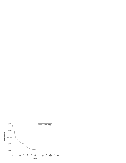
Figure 2: The total energy evolution for case 1.

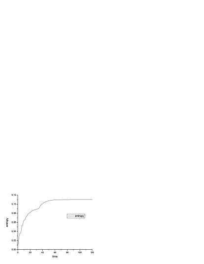
Figure 3: The entropy function evolution for case 1.

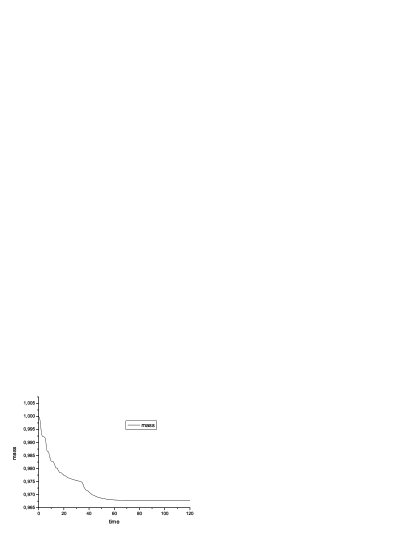
Figure 4: The mass evolution for case 1.

In the second variant of the calculations (see Fig. 5) we set a small initial angular momentum $M_{in}=0.1$. After the collapse, temporary oblate and prolate spheroids appear during the relaxation. There is no secular instability, and the system reaches the equilibrium oblate spheroid of Maclaurin. An initial small difference of parameters connected with axes $a$ and $b$ leads to a small deviation from the results of the similar variant of the 2D simulations (Bisnovatyi-Kogan, 2004). Here we have an additional instability: there is an increase in the difference $(a-b)$ at the early stages of motion. However, this difference remains too small to be visualized in the figure. This is the instability characteristic to the system with purely radial trajectories (Antonov, 1973; Fridman & Polyachenko, 1985). This instability takes place in all variants of the calculations, but in most cases it is very small and always disappears during the relaxation and formation of the equilibrium figure. In the cases of large angular momentum, this instability does not show up because the difference $(a-b)$ quickly increases as a result of secular instability.

To illustrate the radial instability, we consider an initial sphere without rotation ($M_{in}=0$) and without any relaxation process. Only the three equations (15)–(17) with $\tau_{rel}=\infty$ have been used, at constant $m=1$, $M=0$ and $\varepsilon$. We have set small initial differences between the axes $a$, $b$ and $c$, and have obtained an unstable behaviour evidently visible in Fig. 6.

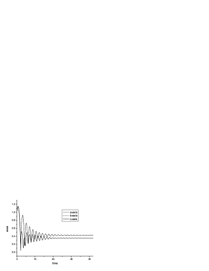
Figure 5: The relaxation to the spheroid at small angular momentum, case 2.

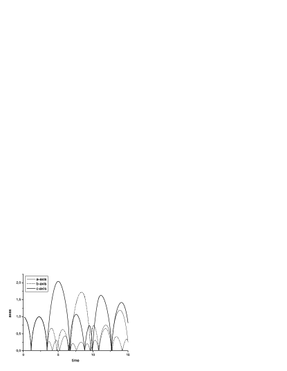
Figure 6: Radial instability development in the non-rotating body, without dissipation, case 3.

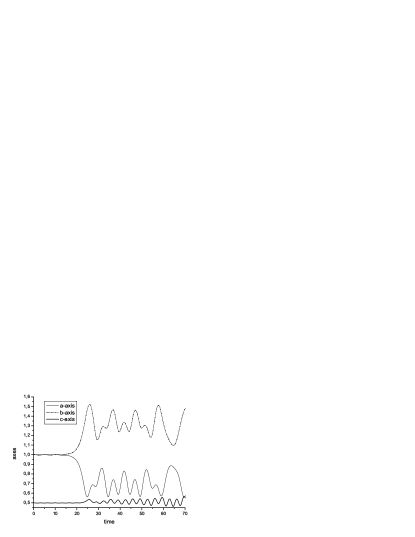
Figure 7: Development of the secular instability in a rapidly rotating body, without dissipation, case 4.

For numerical investigation of the secular instability, we consider equations of motion without dissipation, and take the equilibrium spheroids with small perturbation as the initial configuration. It is easy to obtain the equilibrium parameters of the spheroid from the equations of motion with zero accelerations. The initial equilibrium configuration of the Maclaurin spheroid was slightly perturbed by increasing $b$, as in the last column of Table 1. At small angular momentum we obtain the conservation of the initial configuration. There are small oscillations around the equilibrium spheroid, during which the difference $(a-b)$ changes sign periodically. At large angular momentum we obtain the development of the secular instability, and, after several low-amplitude oscillations, the Maclaurin spheroid, is transformed into the Jacobi ellipsoid (see Fig. 7 where the variant with large angular momentum is represented). Because of the absence of relaxation, the system does not reach an equilibrium configuration and oscillations continue. If we include relaxation in this variant, we should observe the final equilibrium state of the ellipsoid. Our calculations allow us to find approximately numerically the point of the onset of the secular instability of a compressible Maclaurin spheroid. It fits well with the analytical results obtained in the next section.

6 Equilibrium configurations and stability

Equilibrium of a uniformly rotating figure (spheroid or ellipsoid) is found from the equations (15)–(17) with zero time derivatives:

$$0=-\frac{3m}{2}\,a\int\limits_{0}^{\infty}\frac{du}{(a^{2}+u)\Delta}\,\,+\,\frac{10}{3m}\,\frac{1}{a}\,\frac{\varepsilon}{(abc)^{2/3}}\,\,+\frac{25M^{2}}{m^{2}}\,\frac{a}{(a^{2}+b^{2})^{2}}\,,$$ (26)

$$0=-\frac{3m}{2}\,b\int\limits_{0}^{\infty}\frac{du}{(b^{2}+u)\Delta}\,\,+\,\frac{10}{3m}\,\frac{1}{b}\,\frac{\varepsilon}{(abc)^{2/3}}\,\,+\frac{25M^{2}}{m^{2}}\,\frac{b}{(a^{2}+b^{2})^{2}}\,,$$ (27)

$$0=-\frac{3m}{2}\,c\int\limits_{0}^{\infty}\frac{du}{(c^{2}+u)\Delta}\,\,+\,\frac{10}{3m}\,\frac{1}{c}\,\frac{\varepsilon}{(abc)^{2/3}}.$$ (28)

Introducing the variables

$$x=\frac{u}{a^{2}},\quad k=\frac{c}{a},\quad k_{1}=\frac{b}{a},\quad j=\frac{M}{m},\quad\epsilon=\frac{\varepsilon}{m},$$ (29)

and integrals

$$I_{1}(k,k_{1})=\int_{0}^{\infty}\frac{dx}{(x+1)^{3/2}\sqrt{(k_{1}^{2}+x)(k^{2}+x)}}\,,\quad I_{2}(k,k_{1})=\int_{0}^{\infty}\frac{dx}{(x+k_{1}^{2})^{3/2}\sqrt{(1+x)(k^{2}+x)}}\,,$$ (30)

$$I_{3}(k,k_{1})=\int_{0}^{\infty}\frac{dx}{(x+k^{2})^{3/2}\sqrt{(1+x)(k_{1}^{2}+x)}}\,,$$

we can write equations (26)-(28), using (19), in the form

$$0=-\frac{3m}{2}\,a\,I_{1}(k,k_{1})+\,\frac{10}{3}\,\frac{\epsilon}{(kk_{1})^{2/3}}\,\,+\frac{25j^{2}}{(1+k_{1}^{2})^{2}}\,,$$ (31)

$$0=-\frac{3m}{2}\,ak_{1}\,I_{2}(k,k_{1})+\,\frac{10}{3}\,\frac{\epsilon}{k_{1}(kk_{1})^{2/3}}\,\,+\frac{25j^{2}\,k_{1}}{(1+k_{1}^{2})^{2}}\,,$$ (32)

$$0=-\frac{3m}{2}\,ak\,I_{3}(k,k_{1})+\,\frac{10}{3}\,\frac{\epsilon}{k(kk_{1})^{2/3}}.$$ (33)

Excluding $m$, we obtain

$$0=-\frac{1}{k^{2}}\frac{I_{1}(k,k_{1})}{I_{3}(k,k_{1})}+1+\frac{15j^{2}}{2\epsilon}\frac{(kk_{1})^{2/3}}{(1+k_{1}^{2})^{2}}\,,\quad 0=-\frac{k_{1}^{2}}{k^{2}}\frac{I_{2}(k,k_{1})}{I_{3}(k,k_{1})}+1+k_{1}^{2}\frac{15j^{2}}{2\epsilon}\frac{(kk_{1})^{2/3}}{(1+k_{1}^{2})^{2}}.$$ (34)

At $a=b$, $k_{1}=1$ equations (34) are identical, and determine the equilibrium of the Maclaurin spheroid (see Bisnovatyi-Kogan 2004). For Jacobi ellipsoids with $a\neq b\neq c$, we obtain the following relation between $k$ and $k_{1}$:

$$F(k,k_{1})=1-\frac{1}{k_{1}^{2}}+\frac{1}{k^{2}}\frac{I_{2}(k,k_{1})}{I_{3}(k,k_{1})}-\frac{1}{k^{2}}\frac{I_{1}(k,k_{1})}{I_{3}(k,k_{1})}=0.$$ (35)

This equation has a trivial solution $k_{1}=1$ at all $k$, corresponding to the Maclairin spheroid. Let us find the bifurcation point of the equation (35), at which non-trivial solutions appear. While $k_{1}=1$ is always a root of equation (35), we may write $F(k,k_{1})=(k_{1}-1)f(k,k_{1})$. An additional root of the equation $F(k,k_{1})=0$ appears when the root of the equation $f(k,k_{1})=0$ appears at $k_{1}=1$. The root of the zero derivative equation $F^{\prime}_{k_{1}}(k,k_{1})=f(k,k_{1})+(k_{1}-1)f^{\prime}_{k_{1}}(k,k_{1})=0$ at $k_{1}=1$ coincides with the root of the equation $f(k,1)=0$. Therefore the value of $k$ at the bifurcation point is determined by the equation

$$\frac{\partial F(k,k_{1})}{\partial k_{1}}|_{k_{1}=1}=0.$$ (36)

Using (30) and (35), this equation is written in the form

$$2k^{2}\,I_{3}(k,k_{1})|_{k_{1}=1}+\frac{\partial I_{2}(k,k_{1})}{\partial k_{1}}|_{k_{1}=1}-\frac{\partial I_{1}(k,k_{1})}{\partial k_{1}}|_{k_{1}=1}=0$$ (37)

At $k_{1}=1$ we have analytic expressions

$$\frac{\partial I_{1}(k,k_{1})}{\partial k_{1}}|_{k_{1}=1}=-I_{0},\quad\frac{\partial I_{2}(k,k_{1})}{\partial k_{1}}|_{k_{1}=1}=-3I_{0},\quad I_{0}=\int_{0}^{\infty}\frac{dx}{(1+x)^{3}\sqrt{k^{2}+x}}\,,$$ (38)

so that the equation (37) is reduced to

$$k^{2}\,I_{3}=I_{0},\quad{\rm where}\,\,\,I_{3}=I_{3}(k,1)\quad{\rm and}\,\,\,I_{2}=I_{2}(k,1)=I_{1}=I_{1}(k,1).$$ (39)

Taking the integrals $I_{0},\,\,I_{1}=I_{2}$ and $I_{3}$ analytically, we have

$$(1-k^{2})I_{0}=\frac{3}{4}I_{2}-\frac{k}{2}\,,\quad I_{3}=\frac{2}{k(1-k^{2})}\biggl{(}1-\frac{k\arccos{k}}{\sqrt{1-k^{2}}}\biggr{)},\,\quad I_{1}=I_{2}=-\frac{1}{k(1-k^{2})}\biggl{(}k^{2}-\frac{k\arccos{k}}{\sqrt{1-k^{2}}}\biggr{)}.$$ (40)

Using (40) in (39) we obtain the equation

$$\frac{\arccos k}{\sqrt{1-k^{2}}}=\frac{k(13-10k^{2})}{3+8k^{2}-8k^{4}}\,,$$ (41)

for which the solution $k=0.582724$ determines the bifurcation point at the sequence of the Maclaurin spheroids. For the uniform spheroid, the position of this point does not depend on the adiabatic index of the matter.

Above, we have obtained the bifurcation point on the equilibrium curve of the Maclaurin spheroids using only the equilibrium relations for the Jacobi ellipsoids. The usual way of investigating stability is to solve linearized equations of motion and to find the eigenfrequencies. The linearized equations (15)–(17) without violent relaxation reduce, with account of (29), to the following form:

$$\delta(\ddot{a}-\ddot{b})=3\frac{m}{a^{3}}\,\left[-k^{2}\int\limits_{0}^{\infty}\frac{du}{(1+u)(k^{2}+u)^{3/2}}\,+\int\limits_{0}^{\infty}\frac{du}{(1+u)^{3}(k^{2}+u)^{1/2}}\right]\delta(a-b)\,.$$

The $\varepsilon$, $U_{tot}$, $m$ and $M$ losses are quadratic to perturbations, so these values remain constant in linear approximation. Taking $\delta(a-b)\sim\exp(-i\omega t)$, we come to the characteristic equation

$$\omega^{2}=3\frac{m}{a^{3}}\,\left[k^{2}\int\limits_{0}^{\infty}\frac{du}{(1+u)(k^{2}+u)^{3/2}}\,-\int\limits_{0}^{\infty}\frac{du}{(1+u)^{3}(k^{2}+u)^{1/2}}\,\right].$$ (42)

The plot $\omega^{2}(k)$ at $m=a=1$ is given in Fig. 8. Using the notations of (38) and (39) in (42), we write the characteristic equation in the form

$$\omega^{2}=3\frac{m}{a^{3}}\,(k^{2}\,I_{3}-I_{0}).$$ (43)

Figure 8: Dependence of the squared eigenfrequency $\omega^{2}$ on the axis ratio $k$ in the Maclaurin spheroid without dissipation terms in the approximate equations of motion.

We see that a spheroid loses its stability for the transformation into a three-axial ellipsoid, at the bifurcation point $k=0.58272$, $e=\sqrt{1-c^{2}/a^{2}}=0.81267$. By derivation it is clear that the position of this point does not depend on the polytropic exponent $n$. Our approximate equations, even without dissipation, describe uniformly rotating ellipsoids (spheroids), which are not connected by adiabatic relations, and contain a ”hidden” non-conservation of the local angular momentum, which preserves the uniformity. Therefore, in the presence of this ”hidden” non-conservation, the loss of stability takes place exactly at the bifurcation point. The loss of stability is not connected with relaxation and follows from our equations even in the case when all the global integrals remain constant. In the exact approach, the instability at this point happens only in the direct presence of dissipative terms (Chandrasekhar, 1969). The pure adiabatic spheroidal system preserves stability until $e=0.952887$, where it becomes unstable via a vibrational mode.

In our approach we cannot exactly investigate the effect of pure bulk viscosity on the stability of the compressible spheroids, because the transition is influenced by the hidden non-conservation. Taking account of bulk viscosity and violent relaxation does not change the bifurcation point. However, in some cases the presence of relaxation has a stabilizing influence on the motion of the system.

We have considered an equilibrium configuration of the Maclaurin spheroid close to the bifurcation point, in the interval of the secular instability. After perturbation of the density, the spheroid starts to oscillate. Our calculations have shown that in the absence of relaxation the development of instability and the transition of the spheroid to a three-axis object both occur. In the presence of relaxation the perturbed spheroid remains a spheroid and the system reaches the equilibrium state. This behaviour takes place because during relaxation the thermal energy increases, and the eccentricity $e$ decreases and comes into the interval of stability. So the spheroid initially perturbed in the interval of instability, not far from the bifurcation point, becomes stable due to the processes of relaxation.

According hypothesis of Ostriker & Peebles (1973), the stability of an isolated axially symmetric system is determined by the ratio $U_{rot}/|U_{g}|$. They determined from numerical experiments the critical value for various configuration as $0.14\pm 0.03$. Shapiro (2004) found that compressible spheroids become secularly unstable to triaxial deformations at the bifurcation point, where $U_{rot}/|U_{g}|=0.1375$, independent of $n$. Our formula gives exactly the same result, which is also confirmed by our numerical simulations. As noted above, this result remains valid also in the presence of dissipation.

7 Conclusions

We have investigated the dynamics of a three-axis dark matter ellipsoid. The equations of motion for the axes of a uniform compressible ellipsoid have been obtained by variation of the Lagrange function, in which violent relaxation and losses of matter, energy and angular momentum have been included phenomenologically.

The system was solved numerically, until the formation of stationary rotating figures in the presence of relaxation. For lower angular momentum $M$ we have the formation of a compressed spheroid, while at larger $M$ we follow the development of a three-axial instability and the formation of a three-axial ellipsoid. The instability in this approximation happens at the bifurcation point of the sequence of Maclaurin spheroids, where the Jacobi ellipsoidal system starts.

The bifurcation point coinciding with the point of loss of stability is found analytically in the form of a simple formula, by static and dynamic approaches. Numerical and analytical considerations give identical results.

The development of instability, connected with radial orbits, is obtained for slowly rotating collapsing bodies.

References

• Antonov (1973) Antonov V.A., 1973, in Omarov G. B., ed., The Dynamics of Galaxies and Stellar Clusters. Nauka, Alma-Ata (in Russian), p.139
• Bisnovatyi-Kogan (2004) Bisnovatyi-Kogan G.S., 2004, MNRAS, 347, 163
• Chandrasekhar (1969) Chandrasekhar S., 1969, Ellipsoidal Figures of Equilibrium. Yale Univ. Press, New Haven, CT
• Fridman & Polyachenko (1985) Fridman A.M., Polyachenko V.L., 1985, Physics of Gravitating Systems. Springer Verlag, Berlin
• Fujimoto (1968) Fujimoto M., 1968, ApJ, 152, 523.
• Gradshtein & Ryzhik (1962) Gradshtein I.S., Ryzhik I.M., 1962, Table of Integrals, Sums, Series, and Products. Fizmatgiz, Moscow
• Lai, Rasio & Shapiro (1993) Lai D., Rasio F.A., Shapiro S.L., 1993, ApJS, 88, 205
• Lai et al. (1994a) Lai D., Rasio F.A., Shapiro S.L., 1994, ApJ, 423, 344.
• Lai, Rasio & Shapiro (1994b) Lai D., Rasio F.A., Shapiro S.L., 1994, ApJ, 437, 742.
• Landau & Lifshitz (1993) Landau L.D., Lifshitz E.M., 1993, The Classical Theory of Fields. Pergamon, Oxford
• Lin, Mestel & Shu (1965) Lin C.C., Mestel L., Shu F.H., 1965, ApJ, 142, 1431.
• Lynden-Bell (1964) Lynden-Bell D., 1964, ApJ, 139, 1195.
• Lynden-Bell (1965) Lynden-Bell D., 1965, ApJ, 142, 1648.
• Lynden-Bell (1967) Lynden-Bell D., 1967, MNRAS, 136, 101.
• Lynden-Bell (1979) Lynden-Bell D., 1979, The Observatory, 99, 89.
• Lynden-Bell (1996) Lynden-Bell D., 1996, Current Science, 70, 789.
• Ostriker & Peebles (1973) Ostriker J.P., Peebles P.J.E., 1973, ApJ, 186, 467
• Rosensteel & Huy (1991) Rosensteel G., Huy Q.T., 1991, ApJ, 366, 30
• Shapiro (2004) Shapiro S.L., 2004, ApJ, 613, 1213.
• Zel’dovich (1970) Zel’dovich Ya.B., 1970, Afz, 6, 119