11email: wfh@mpa-garching.mpg.de 22institutetext: Universität Würzburg, Am Hubland, D-97074 Würzburg, Germany
22email: [luigi,niemeyer]@astro.uni-wuerzburg.de 33institutetext: International University Bremen, Campus Ring 1, D-28759 Bremen, Germany
33email: m.brueggen@iu-bremen.de
The ignition of thermonuclear flames in Type Ia supernovae
In the framework of the Chandrasekhar-mass deflagration model for Type Ia supernovae (SNe Ia), a persisting free parameter is the initial morphology of the flame front, which is linked to the ignition process in the progenitor white dwarf. Previous analytical models indicate that the thermal runaway is driven by temperature perturbations (“bubbles”) that develop in the white dwarf’s convective core. In order to probe the conditions at ignition (diameters, temperatures and evolutionary timescales), we have performed hydrodynamical 2D simulations of buoyant bubbles in white dwarf interiors. Our results show that fragmentation occurring during the bubble rise affects the outcome of the bubble evolution. Possible implications for the ignition process of SNe Ia are discussed.
Key Words.:
Supernovae: general – Hydrodynamics – Methods: numerical – White dwarfs1 Introduction
Advances in computer simulations of type Ia supernovae (SN Ia) have led to a rough consensus over the nature of these explosions, even if several issues remain controversial. SNe Ia are believed to be the outcome of thermonuclear explosions of carbon-oxygen white dwarfs (CO WDs) in binary systems. Among possible explosion scenarios (see Hillebrandt & Niemeyer 2000 for a review of them) the single degenerate scenario fares best in explaining the observed homogeneity of SNe Ia (Leibundgut 2000). In this model a CO WD approaches the Chandrasekhar mass by mass transfer from a non-degenerate companion and is disrupted by a thermonuclear explosion.
In this paper we wish to study the processes that lead to the ignition of SNe Ia. The mechanism that ignites the thermonuclear flame in the WD core is the link between the late stages of the progenitor evolution and the development of the initial flame morphology. From a practical point of view, it provides the initial conditions for the explosion simulations. A large set of different initial conditions has been tested in the literature of SN Ia simulations, with results ranging from mildly energetic (Reinecke et al. 2002b; Gamezo et al. 2003; Travaglio et al. 2004; Röpke & Hillebrandt 2005) to failed explosions (Calder et al. 2004) in pure deflagration explosion models. The initial flame setup in multi-dimensional simulations of SN Ia explosions is considered basically a free parameter, though constrained by some analytical works (García-Senz & Woosley 1995; Woosley et al. 2004; Wunsch & Woosley 2004; Sect. 2.2). Consequently most simulation schemes are tested against different sets of initial flame shapes, allowing a comparison of the results for various setups (Reinecke et al. 2002b; Röpke & Hillebrandt 2005; García-Senz & Bravo 2005; Livne et al. 2005).
Among the possible initial conditions the most intuitive one, also for its use in 1D simulations, is the centrally ignited flame (e.g. Niemeyer & Hillebrandt 1995; Reinecke et al. 1999, 2002a; Gamezo et al. 2003). A different ignition condition is provided by a number of spherical flame kernels placed in the innermost part of the WD and detached from the center. Early works in 2D (Niemeyer et al. 1996; Reinecke et al. 1999) implemented only a few blobs per quadrant, while newer simulations (Reinecke et al. 2002b; Travaglio et al. 2004) have a finer spatial resolution and allow the implementation of more seeds. Nevertheless, the maximum number of blobs that constitute the initial flame is still constrained by resolution rather than physics. This situation may be cured by the use of co-expanding computational grids (Röpke 2005). A hybrid approach between centrally ignited flame and multi-spot scenario is presented by Röpke & Hillebrandt (2005) in a full-star 3D simulation.
The influence of different initial conditions on the outcome of the explosion has been discussed in several papers. There is general agreement that an initially larger number of blobs produces more vigorous explosions because the initial flame surface is relatively larger and can provide more flame acceleration. Also the comparison of different initial conditions in Röpke & Hillebrandt (2005) shows that the hybrid “foamy” initialization provides more seeds for the development of instabilities and gives a larger total energy and production of with respect to the model ignited at the center. In the same work, the comparison with the failed explosion found by Calder et al. (2004) is addressed. Their simulation starts from a single spherical flame seed, displaced slightly off-center.
Since the features of SN Ia explosions depend on the number of igniting points in the WD core, an interesting question pertains to an estimate of this number. In the papers cited above the study of this problem was conducted by means of an a posteriori evaluation of the explosion features as a function of the initial conditions, without exploring the physics of the ignition process itself (with the exception of Woosley et al. 2004). A successful ignition theory has to provide a physical basis for the choice of favored initial conditions in SNe Ia explosion models.
In this paper, a new approach to the ignition problem is based on 2D simulations performed with the FLASH code (Fryxell et al. 2000). We will use an indirect approach: the features of the ignition process will be explored by studying temperature perturbations in the WD core (“bubbles”) that are supposed to trigger the ignition (cf. Sect. 2.2). Using the results of the bubble simulations, we are able to obtain important clues about the ignition physics.
The paper is structured as follows: in Sect. 2 the basic ideas of the physics of ignition are introduced. Section 3 describes the setup of the simulations. Section 4 focuses on the bubbles, presenting the relevant physics and the issues related to the 2D simulations. Some important parameters for the bubble evolution are highlighted and their role is explored in Sect. 5. In Sect. 6 we use the results of the simulations in order to study possible implications for the ignition of SNe Ia. Our conclusions are summarized in Sect. 7.
2 The ignition process of SNe Ia
2.1 Final stage of the progenitor evolution
According to stellar evolution models, CO WDs are the endpoints of the evolution of main sequence stars in the mass range (Umeda et al. 1999). The energetics in the WD’s interior during the accretion phase is determined by the following processes:
-
•
Compressional heating caused by accretion, described in detail e.g. by Iben (1982).
-
•
Nuclear burning: Compression and heating trigger hydrostatic carbon burning in the WD core. According to Nomoto (1982) the burning starts in the pycnonuclear regime and turns to the thermonuclear regime for .
-
•
Neutrino emission: The energy loss by neutrino emission is important at densities below about (Arnett 1971; Nomoto et al. 1984; Woosley & Weaver 1986). In these conditions, the dominant contribution to neutrino losses comes from the production of plasmon neutrinos, a mechanism described for example by Clayton (1983) and Winget et al. (2004). As a result of accretion, the density increases above , the thermal photons do not have enough energy for plasmon excitation and the neutrino production in the WD core is strongly suppressed.
In the evolutionary plane of central density and temperature () (cf. Yoon & Langer 2003), the locus where the energy release due to carbon burning is equal to the energy loss by neutrino emission is traditionally referred to as the “ignition line”. Actually it marks the start of the last phase of the progenitor evolution. In order to get rid of the energy output of the carbon burning, the WD develops a convective core whose evolution is crucial for the knowledge of the ignition properties. The duration of the convective phase is of the order of years (Hillebrandt & Niemeyer 2000; Yoon & Langer 2003).
When the core temperature reaches , the convective zone encompasses most of the WD mass. Convection enters a reactive regime (Woosley et al. 2004), in which the convective turnover timescale and the nuclear timescale , defined as the time required to significantly reduce the carbon abundance in an isolated region of the fluid, are comparable. At the critical temperature (Timmes & Woosley 1992) for carbon burning is reached, i.e. the temperature where the energy generation rate is equal to the heat conduction rate. This point defines the start of the SN Ia explosion, the ignition of the thermonuclear runaway.
Beyond the description of this sequence of events, a consistent ignition model of SNe Ia is required to answer more detailed questions. In particular, the initial location and morphology of the flame in the WD, the time evolution of the ignition process and the thermodynamic state of the WD core prior to runaway need to be explored. One possible approach to study the multi-dimensional features of reactive convection is a direct numerical simulation of this phase. A 2D simulation performed with an implicit code and limited to the last few hours before the runaway was performed by Höflich & Stein (2002). According to the results of this work, the ignition occurs at the center of the WD and is triggered by compressional heating in the convective flow. These conclusions were challenged by Woosley et al. (2004) who claim that the central ignition was either an artifact caused by the forced symmetry of the 2D simulation, or caused by insufficient resolution.
2.2 Temperature fluctuations in the WD core
The idea that the SN Ia explosion is ignited by floating bubbles has been proposed first by García-Senz & Woosley (1995). The formation of these temperature fluctuations in the WD’s convective core is connected to the turbulent behavior of the WD fluid and can be explained in terms of velocity fluctuations. Wunsch & Woosley (2004) show that, when a fluid element, during the convective motion, approaches the energy generating core of the WD111Considering the high sensitivity of the C-burning rate on temperature, it may be proved (Woosley et al. 2004) that one half of the energy is produced in a small (estimated mass of , corresponding to about for the WD model examined by those authors) central part of the convective core. with a velocity smaller than the average convective velocity, it stays there for a slightly longer time than average and becomes hotter (and less dense) than the surrounding material. Therefore, the bubble is subject to buoyancy and rises from the center of the WD.
The rising bubbles play a key role in the ignition because they are regarded as the “seeds” for the subsequent flame propagation. The initial flame in the progenitor is determined by motion of the bubbles inside the convective core. The study of the bubble features is an important part of investigating the ignition process.
García-Senz & Woosley (1995) have developed an analytic model for the buoyant evolution of burning bubbles. They have performed a parameter study in which they investigate the bubble motion as a function of the initial bubble position, the diameter, and the initial temperature excess. The conclusion is that the bubbles reach the runaway temperature when they are at a central distance in the range , moving with a speed of about .
The topic has been revisited by Woosley et al. (2004). On the topic of ignition they conclude that it is initiated by bubbles at a central distance of up to about , when the central WD temperature is about . Moreover, they claim that a multi-point ignition is possible. This results from the fact that the e-folding timescale for the number of bubbles is comparable with the time for the expansion in the SN Ia explosion to shut off the ignition ().
Finally, the ignition has been addressed in a more general, heuristic model of turbulent convection by Wunsch & Woosley (2004). Two convective flow patterns are considered, an isotropic turbulent flow and a dipolar jet flow. As far as the central WD temperature is concerned, the conclusions for the SN ignition are similar to previous work. On the location of the hottest points in the WD the authors consider the competition between nuclear heating and adiabatic cooling and estimate that the ignition points should be concentrated at about 100 km from the WD center. For an isotropic flow it means that the ignition points should occur in a shell of 100 km of diameter while for a dipole flow these points would be clustered rather along the flow axes.
3 Numerical tools
The 2D simulations which we will present here have been produced using FLASH (version 2.3), a parallel adaptive-mesh hydro code (Fryxell et al. 2000). The FLASH code has been used, among other topics, for the study of SN Ia explosions (Calder et al. 2004; Plewa et al. 2004) and, in a different context, also in the study of the morphology of rising bubbles (Robinson et al. 2004; Brüggen et al. 2005a, b) in cooling flows in galaxy clusters.
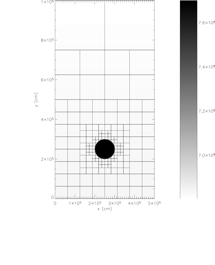
Figure 1 shows the computational domain at the beginning of a 2D bubble simulation. As explained below, the computational domain encloses only a small part of the WD. In this domain the bubble is set at rest. Since most of the calculations are performed with bubbles of in diameter, the following description will refer to this case (for different bubble diameters one just has to scale the lengths accordingly).
The size of the computational domain is . The bubble is initialized as a temperature perturbation in pressure equilibrium with the surrounding matter. The values of the thermodynamical variables in the domain are obtained from a one-dimensional WD model provided by S. Woosley, with mass , radius , , . The extent of the convective zone in the model is about 1000 km.
Since the computational domain encloses a relatively small part of the WD, a reasonable approach is to neglect the effect of curvature and to map the data from the WD model in a plane-parallel approximation. The values of physical quantities on the computational grid at coordinate are taken from the quantities in the WD model at the radius , where is the parameter which expresses the initial distance of the bubble from the WD center and is the coordinate of the bubble center in the computational domain. Before initialization, the pressure and density data are slightly modified to ensure the hydrostatic equilibrium, as described by Zingale et al. (2002). A spatially constant gravitational force, computed from the WD model, is applied to the computational domain. This assumption is not strictly valid because the variation of the gravitational acceleration along the whole computational domain (20 km) is relevant. However, we do not expect this to affect our results since the extent of the bubble motion is always smaller than the computational domain, namely of the order of a few kilometers (Fig. 2), comparable with the bubble diameter. The boundary conditions are set to be reflecting in the upper and lower boundaries, and periodic in the -boundaries.
The simulations are performed in 2D Cartesian geometry. In principle, this is not the most natural choice of geometry since a bubble is a spherical object and it would be better represented in 2D in cylindrical coordinates, exploiting the axial symmetry. Nevertheless, some tests have been performed, both, in 2D Cartesian and cylindrical geometry. Simulations in cylindrical geometry present special difficulties, with respect to the Cartesian geometry, because of larger numerical dispersion (cf. Sect. 4.3) and the appearance of “axis jets” which distort the bubble morphology. The tests show that the choice of the Cartesian geometry is acceptable for following the thermal evolution of bubbles.
The adaptive mesh refinement implemented in FLASH is apparent in Fig. 1. Resolution tests have shown that a good compromise between computational cost and adequate resolution is to use five levels of refinement yielding an effective grid size of zones (cf. Sect. 4.3). This corresponds to a spatial resolution of at the most resolved level.
Among the different equations of state implemented in FLASH, the Helmholtz EOS described by Timmes & Swesty (2000) was chosen for our setup. In order to follow the hydrostatic carbon burning the small reaction network iso7 was used. This -network is adequate for the physical problem under examination, as confirmed by Timmes et al. (2000).
To date, in the latest publicly available version of FLASH (v. 2.5) there is no treatment of flame propagation. Therefore, the simulations are followed until , which is when the flame is going to start, and are then stopped. Since this work is devoted to the study of the progenitor’s evolution before the runaway starts, this limitation does not concern us much.
4 Two-dimensional simulations of rising bubbles
4.1 List of the performed simulations
In order to cover the broad range of bubble parameters that is likely to exist inside the WD, we present a study that explores the dependence of the bubble evolution on the three main parameters:
-
•
The initial bubble diameter, .
-
•
The initial bubble temperature, .
-
•
The initial distance of the bubble from the WD center, .
The aim of the study is to understand under which (physically meaningful) conditions thermonuclear runaway ensues and what the related timescales are.
| Distance from the | Parameters | |||
| WD center and | of the simulations | |||
| background temperature | ||||
| 7.3 | 7.5 | 7.6 | ||
| Background = 6.96 | ||||
| 7.7, = 5 km | ||||
| 7.3 | 7.5 | 7.7 | 7.9 | |
| Background = 6.83 | 7.7, = 0.2 km | |||
| 7.3 | 7.5 | 7.7 | 7.9 | |
| Background = 6.63 |
The thirteen calculations performed for our parameter study are listed in Table 1. In the first column the central distances of the bubbles are given, together with the background temperature of the WD at that distance from the center (in units of ). In the other four columns, the simulations are identified by the initial temperature, again in units of . The bubble diameter is fixed at 1 km unless explicitly specified. Simulations that reach the thermal runaway are in boldface. To sum up, the initial parameters have been varied in the following way:
-
1.
(bubble diameter): for the case with , , the three values 0.2, 1, 5 km have been tested. The lower limit is constrained by computational feasibility, decreasing the timestep of the simulations together with the spatial resolution because of the CFL condition for the equations of hydrodynamics.
-
2.
(bubble temperature): . The upper end of this range is set in order to avoid too extreme temperature contrasts with respect to the background. For bubble temperatures smaller than the lower end of the range, the nuclear timescale is longer than about 5 s. It seems unlikely that a bubble can have such a long evolution, without being disrupted as described in Sect. 4.3.
-
3.
(distance from the WD’s center): the three values 50, 100, 150 km have been explored. Following Wunsch & Woosley (2004), we assume that the bubbles are produced in the energy generating core of the WD, which extends approximately over this range of central distances.
4.2 Diagnostic quantities
First, we will define some quantities that are useful for the interpretation of our simulations.
A first difficulty in defining these quantities is the lack of a good criterion about the bubble location in the computational domain. This is of course a typical problem, when dealing with an Eulerian system of coordinates. In principle, hot material (the bubble is set to be rather hotter than the background) could keep track of the bubble evolution. Unfortunately, in Sect. 4.3 we show that numerical diffusion hampers this approach and one cannot make safe use of “bubble averaged quantities”. Hence, the description of the thermal evolution of the bubble will be done by studying the maximum temperature in the bubble.
A useful quantity for the following analysis of the bubble is its area. As written above, it is difficult to provide an unambiguous definition of this variable. Test simulations have established that a good criterion is given by the following expression:
| (1) |
where the sum is calculated over the zones where and the threshold temperature is defined by
| (2) |
where is the initial bubble temperature. The quantity is geometry dependent. In Cartesian geometry it can be simply identified with the zone area , where and are the zone sizes in the two directions.
It is also useful to introduce the effective gravitational acceleration (García-Senz & Woosley 1995; Woosley et al. 2004). The acceleration exerted by buoyancy on a rising bubble is proportional to its density contrast:
| (3) |
In the previous equation, the density contrast between the bubble and the background can be expressed in terms of the temperature contrast times , the logarithmic derivative of density with respect to temperature at constant pressure.
4.3 The physics of the bubble
There exists an extensive literature on the fluid mechanics of rising bubbles. Nonetheless, we are not aware of any work that addresses the peculiarities of the present setup (degenerate matter, very small density contrasts and nuclear burning).
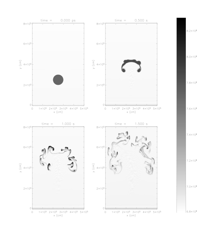
At first, our discussion will focus on the following “reference choice” of parameters: initial temperature , initial diameter , initial central distance (Fig. 2). These values have been chosen to lie well inside the range of variation of the three parameters, discussed in Sect. 4.1 and also suggested by Woosley et al. (2004). First we will describe the results for these reference parameters, while in Sect. 5 we will explore the results of varying these parameters.
If we neglect adiabatic cooling (as motivated in Sect. 6.1), the evolution of the bubble depends only on the interplay between nuclear burning and hydrodynamical instabilities.
Hydrostatic carbon burning sets the timescale for the bubble to reach the thermonuclear runaway. This nuclear timescale (Woosley et al. 2004) has been introduced in Sect. 2.1. Using the evolutionary timescales of the simulations that reach a runaway (cf. Table 1) and adding data from further tests an analytical fit to has been found. The result is
| (4) |
where and . This fit of is in rough agreement with the derivation by Woosley et al. (2004) for the conditions of interest in the WD core.
The bubble motion is a special case of a system subject to the Rayleigh-Taylor instability (in the following, RTI). In a gravitational field with the vector of gravitational acceleration pointing downwards along the -axis, the hotter and lighter fluid accelerates upwards. The development of the RTI and the features of the motion in this situation have been addressed in several works (Davies & Taylor 1950; Taylor 1950; Layzer 1955; Glimm & Li 1988; Li 1996). A crucial parameter in this problem is the Atwood number ,
| (5) |
where and are the bubble and background densities, respectively. In our bubble problem, the density contrast is very small because of the degeneracy of the WD matter, and is of the order of . Theory predicts that the rise velocity of the bubble tends to a value that is determined by the equilibrium between buoyancy and drag forces. An analytical model developed for nonlinear, single-mode, classical RTI at arbitrary Atwood number by Goncharov (2002) provides the estimate
| (6) |
where is the wavenumber of a perturbation of size of order of the bubble radius , and is a numerical constant whose value is 3 in 2D and 1 in 3D. From Eq. (6) one gets, for the reference choice of bubble parameters, . This is an appropriate order-of-magnitude estimate for the bubble velocity in the simulations, even if the morphology evolution of the bubble prevents a more quantitative analysis.
The vortical motions produced during the bubble rise cause its fragmentation as it is clear from Fig. 2. In the nonlinear stage of the RTI a large variety of phenomena can account for the observed fragmentation, as described e.g. by Abarzhi et al. (2003) and reviewed by Nakai & Takabe (1996) in the framework of inertial confinement fusion. We will not address a detailed study about the nature of these secondary instabilities. The features of the fragmentation process and some related numerical issues are described below.
An approximate estimate for the timescale of the fragmentation process can be given by defining a dispersion timescale
| (7) |
which, with the reference values of the parameters and the use of eq. (6), gives a timescale of about , a sort of “bubble lifetime”, to be compared with the morphological behavior shown in Fig. 2.


During the fragmentation, the typical length scale of the bubble fragments decreases in time. From a physical point of view, one can expect that the dispersion goes on until the typical length scale of a bubble part is comparable with the minimum size , defined as the diameter of the bubble in which the heat generated by nuclear burning is balanced by heat diffusion. An evaluation of this quantity is performed, with different derivations, by Woosley et al. (2004) and García-Senz & Bravo (2005), and gives results in the range .
For bubbles whose size is larger than , the nuclear heating is larger than the heat loss by conduction. In these bubbles the temperature increases (in this phase, in principle, they can still reach and trigger the thermonuclear runaway), until disruption causes their typical size to decrease to . Then they begin to cool down. Thus, the trend of the maximum temperature shown in Fig. 3 can be easily interpreted: the bubble is heated until either runaway occurs or the bubble is disrupted.
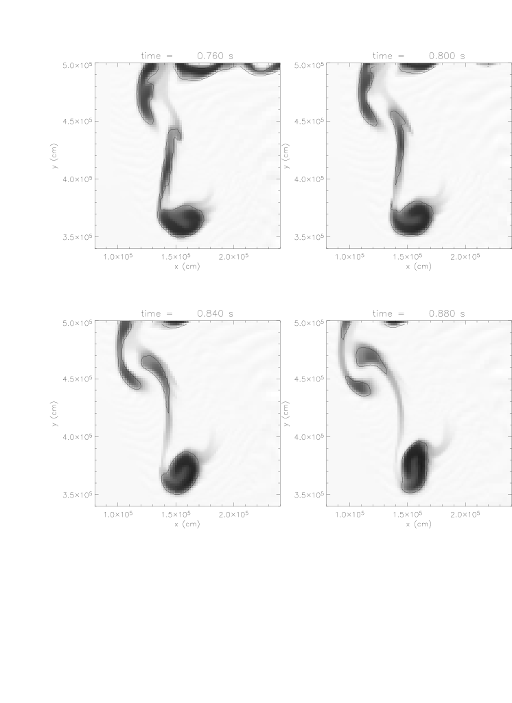
One should note, however, that the length scale for dispersion driven by heat conduction is much smaller than the spatial resolution of the simulations (). is so small that a direct simulation to that scale, even with AMR, is not feasible. What is actually observed in the bubble simulations is not a physical but a numerical dispersion. Figure 5 is meant to clarify this important point. The plots are zoomed on a small detail, a sort of “bridge” linking the top of the bubble with a lower vortical structure. This detail becomes thinner and, as its width is approximately 2–3 times the spatial resolution, it cools off unphysically. It is thus lost from the bubble area according to the definition in Sect. 4.2.
The dependence of the bubble fragmentation process on resolution is shown in Fig. 3. As expected, the numerical dispersion depends on spatial resolution, and the temperature decrease occurs earlier for the simulation with coarser level of refinement. The resolution which has been chosen for the parameter study (five levels of refinement) guarantees however to follow reliably the fragmentation process, as shown in Fig.4. Interestingly, the area evolution in the two most resolved simulations does not show any significant dependence of the bubble area decrease on the level of refinement of the simulation. Probably, this happens because the hydrodynamical instabilities in the more resolved calculation produce structures that are globally more numerous, though smaller in size.
As described above, electron conduction is an important ingredient in the bubble physics, but can be neglected at the length scales which are explored in this study. It is known from the theory of thermonuclear combustion (see e.g. Timmes & Woosley 1992) that heat exchange can inhibit the growth of instabilities which are smaller than a minimum length scale . According to Timmes & Woosley (1992),
| (8) |
where is the modulus of the gravitational acceleration and is the density contrast of the bubble with respect to the background. The flame velocity can be meaningfully replaced, in the case of volume burning, by . In the case under examination (, ) the typical values of the quantities in Eq. (8) are (cfr. Sect. 4.3) , , and . This estimate shows that is of the order of . It is smaller than , therefore the described bubble physics is not affected by the stabilization.
4.4 Outcome of the bubble evolution
The following overview sums up the main features of the bubble evolution:
-
•
The initial bubble temperature determines the nuclear timescale (Eq. 4). This is the upper limit for the duration of the bubble evolution.
-
•
The bubble is fragmented during its motion on a timescale approximately given by (Eq. 7). Physically, the dispersion proceeds down to length scales where heat conduction is effective in dissipating the energy generated by nuclear burning.
-
•
The previous argument is made more complicated by numerical diffusion. It is not possible to quantify exactly the whole duration of the physical dispersion phase described previously because this process can be followed in the simulations only until the typical length scale of the bubble substructures are comparable to 2–3 times the spatial resolution.
The competition between nuclear heating and dispersion is the key to understand the outcome of the bubble evolution and, consequently, also to the ignition process of SNe Ia. Roughly speaking, if is smaller than the burning prevails and the bubble reaches the thermonuclear runaway. Conversely, if the bubble is disrupted and cools down. Analytical studies on ignition that is driven by floating bubbles have not explored the bubble dispersion (García-Senz & Woosley 1995; Woosley 2001; Woosley et al. 2004; Wunsch & Woosley 2004).
4.5 Background turbulence
In all our simulations the background state of the WD was assumed to be “quiet” and in hydrostatic equilibrium. However, the convective flow in the WD prior to runaway is turbulent, with an estimated Reynolds number about (Woosley et al. 2004). The integral length scale , at which the turbulent kinetic energy is injected, is given by the pressure scale height, about for the WD model used here (Woosley 2001). Assuming Kolmogorov scaling for the typical velocity of the convective eddie of length scale , the characteristic turbulent velocity at this length scale is expressed by .
In our case, (spatial resolution of the simulation at the most resolved level) and is in the range , from estimates based on mixing length theory. Therefore, the typical turbulent velocity is in the range , which is of the same order of magnitude as the typical rise velocity of the bubble, according to Eq. (6). A test simulation, performed by imposing a random velocity field with an amplitude of the order of , shows that this stirring affects the bubble evolution only marginally, contributing to a moderately enhanced bubble disruption. We conclude that this turbulence-induced bubble disruption can be considered a second-order effect in the description of the relevant bubble physics discussed in Sect. 4.3.
Our simulations are affected by numerical dispersion and hence overestimate the bubble disruption and the subsequent bubble cooling. From a physical point of view one expects that the bubble temperature would increase for a longer time than is shown, for example, in Fig. 3. However, the numerical dispersion may not be too unphysical because it may mimic the effect of the turbulent-induced bubble disruption. A qualitative comparison of these two effects cannot be performed with our computational tools.
5 The parameter study
5.1 The effect of the bubble diameter


As outlined in Table 1, the role of different bubble diameters was studied on the basis of three calculations, with initial parameters and . The initial diameter was varied by a factor of five above and below the reference value, i.e. , and . The extent of the computational domain and the spatial resolution were scaled accordingly in order to resolve the initial bubble by an identical number of zones. Figures 6 and 7 present a comparison of the maximum temperature and the normalized bubble area, respectively.
As expected, the bubble diameter affects the dispersion timescales. Indeed, the dispersion timescale (Eq. 7) scales as since, from Eq. (6), as well. This scaling is nicely confirmed by the comparison of the area evolution in Fig. 7. While in the simulation with the area starts to decrease at approximately , one can see that for the bubble with the analogous decrease starts at .
For the same reason, the bubble with has a larger . Since the nuclear timescale does not depend on the bubble diameter, this leads to , and the bubbles goes to runaway.
From this study, one can conclude that the larger bubbles are more likely to go to runaway. However, Woosley et al. (2004) find that turbulent dispersion limits the bubble size in the WD to .
5.2 The effect of the bubble temperature


The initial temperature is the most interesting parameter because its role in the bubble physics is manifold. As shown in table 1, several values have been tested. For sake of simplicity, a discussion will only be presented for the simulations with , and ranging from to , keeping in mind that the inferred trends are valid also for calculations with other central distances. Figures 8 and 9 present a comparative analysis of the evolution of maximum temperature and area.
The nuclear timescale depends on the bubble temperature in a rather steep way (Eq. 4). Also the dispersion timescale depends implicitly on , approximately via the square root of the Atwood number (cf. Eq. 6). varies in the explored temperature range from () to (). In simpler terms, the temperature contrast between the bubble and the surrounding material is linked to the density contrast and hence to the effective gravitational acceleration (Eq. 3). With equal background temperature (i.e. equal central distance ) hotter bubbles experience larger accelerations and thus faster dispersion. On the other hand, the nuclear timescale decreases even faster with temperature. This indicates the existence of a threshold temperature above which a bubble goes into runaway. At the threshold is found to be approximately .
5.3 The effect of the central distance


While the parameter was shown to be the most interesting one for the bubble physics, the central distance is probably the most relevant one for the ignition scenario of SNe Ia. The analysis was performed by comparing three simulations with the initial parameters , and equal to 50, 100 and .
The increase of in the calculations affects the effective gravitational acceleration for two reasons. First, the modulus of the acceleration increases with in the considered range of distances. Second, the temperature profile of the WD is decreasing (the background temperatures at various are given in Table 1). So at equal bubble temperature, the temperature (and density) contrast is increasing with . This implies that the effective gravitational acceleration increases outwards, too.
This effect is evident in the comparison between the timescales of the two extreme cases, and , from the analysis of Figs. 10 and 11. The simulation with goes to thermonuclear runaway. Its area evolution shows an expansion (partly due to a problem of the definition of “bubble area” when the temperature contrast between the bubble and the background is relatively small). On the other hand, as predicted the dispersion timescales of the other simulations are noticeably shorter as increases.
The role of an increasing is also relevant for the value of the threshold temperature at which the bubbles at different initial distances from the center go into runaway. As shown in table 1, the bubble at reaches the ignition temperature during the simulation with , but with even the bubble at is dispersed before reaching the runaway.
6 Discussion
6.1 Further remarks on the physics of rising burning bubbles
One of the most striking differences between the simulations presented here and the first analytic study on bubble evolution by García-Senz & Woosley (1995) is that the latter does not take into account the dispersion of the bubbles. Consequently, in their work the bubble velocity and the path covered during the rise are much larger than in the present study. Moreover, without dispersion the rise times are rather long, up to about 25 seconds.
The rise velocity of the bubbles in the simulations is of the order of (cf. Eq. 6). Because the timescale until the bubbles either go into runaway or are disrupted (1–2 s) is so short, the bubble evolution occurs mostly near their point of origin (Fig. 2). However, the previous argument neglects the convective motions in the WD core.
Placing a bubble at some distance from the WD’s center and letting it rise is a gross simplification because the convective velocity is always much larger (in the range , from estimates based on the mixing length theory) than the simulated buoyant velocity. So it is the convection which determines the motion of the bubbles, rather than the rise velocity. Clearly, the convective flow pattern crucially affects the spatial distribution of bubbles at runaway.
As the bubble is advected by the convection, it may travel over a distance that is long compared to the estimated central distance at ignition, undergoing some cooling (Wunsch & Woosley 2004). The bubble simulations cannot directly address this physical process. In our setup, the bubble is initially at rest and no convective velocities are imposed on the background. As a result the bubble travels only a distance that is small compared to its diameter. One can prove that adiabatic cooling is negligible in this case, as confirmed by test simulations in which the nuclear burning was switched off.
6.2 Implications for the theory of ignition of SNe Ia
In this section, our results are applied to the ignition process in SNe Ia.
First, a rough estimate of the extent of the size of the ignition zone can be made on the basis of bubble lifetimes and convective velocities. Taking the values of and , respectively, one finds that the extent of the motion of the bubbles advected in the convective flow is about . Considering that the size of the energy-producing core is of the order of , an estimate for the distance covered by a rising bubble before it triggers the ignition is of the order of . The uncertainties in the convective velocity (in the range ) and in the initial bubble location inside the WD core lead to some dispersion around this value, which is of the order of (a fraction of the pressure scale height). We note that this estimate is consistent with García-Senz & Woosley (1995), Woosley et al. (2004) and Wunsch & Woosley (2004).
It is clear that our approach for the study of ignition conditions does not allow any conclusions about the departures from central symmetry. This issue has to be studied with other numerical tools. A promising way seems to be the use of 3D anelastic simulations, adopted by Kuhlen et al. (2003) in the study of convective flows in massive stars. Interesting results of this technique, applied to SN Ia progenitors, are presented by Kuhlen et al. (2005). In any case, the present work highlights the importance of the progenitor evolution for the initial conditions of the SN Ia explosion. The convective pattern plays a crucial role in the ignition process. The initial flame location depends mostly on the position of the bubbles, which, in turn, are advected by the convective motions inside the WD.
Another interesting issue is the initial number of igniting points. Though our approach for the study of the ignition process is indirect, some useful hints can be obtained.
In the present parameter study, several values of the initial temperature have been tested without making assumptions concerning the probability distribution function (PDF) of the temperature fluctuations. Woosley et al. (2004) investigate this problem and indicate two possible PDFs, depending on details on the convective mixing in the WD core. In their work the PDF is either exponential or Gaussian. Without making a choice among these two models, from the generation process of the temperature perturbations it is intuitive that bubbles with a relatively large temperature contrast with respect to the background are less likely to be generated.
Here a thought experiment of two different ignition scenarios is useful. In the first case, let a hot bubble () be in the core of a WD with central temperature . The estimated nuclear timescale is about . If this bubble is on the “hot tail” of the temperature PDF, one can assume that the probability of generating other bubbles with this (or hotter) within is not large, while colder bubbles would not have time to reach the runaway temperature. In this scenario, the ignition would occur in one (or a few) igniting points. However, considering that the dispersion in more effective for bubbles of a large temperature contrast with the background, such kind of ignition scenario is likely to fail. If the explosion is not initiated, the WD goes on increasing its central temperature.
The other scenario is directly connected with the previous idea. In this second idealized setup, let the WD have a larger central temperature, , and the temperature fluctuations be relatively mild with respect to the background. Under these assumptions, the estimated of the bubbles is about , a value compatible with multi-spot ignition, since the e-folding time of the number of bubbles in the WD core is about 0.1 s (Woosley et al. 2004). Moreover, these perturbations are not supposed to be very hot compared to the background. The probability for such bubbles to be generated, according to whatever PDF, should be large, allowing the presence of very many of them in the WD core.
From these arguments the multi-point scenario emerges as a good candidate for an ignition model of SNe Ia.
7 Conclusions
We have studied the ignition process in SNe Ia by simulating the evolution of buoyant bubbles in the WD core. After discussing the bubble physics, the role of the relevant parameters was studied by means of a grid of thirteen simulations. This parameter study shows that floating bubbles may either ignite almost in place or be dispersed by fragmentation. The previous results found an application in the study of ignition process in SNe Ia. The discussion in Sect. 6.2 provides some clue that the multi-spot ignition model is the favored one. This bubble distribution is consistent with the initial conditions assumed in many recent 3D simulations of SNe Ia explosions.
As pointed out e.g. by Hillebrandt & Niemeyer (2000), a successful model for SNe Ia should explain, both, the homogeneity of the class and, hopefully as a function of one or few parameters, the diversity of observational features. The present study indicates that the ignition process contributes to the homogeneity of SNe Ia. The explanation comes from examining the second scenario described in Sect. 6.2. According to the PDFs (no matter which one), there is some probability for the occurrence of one (or a few) relatively hot bubble among the the mild temperature fluctuations. In principle, a very hot bubble could lead to a runaway before the colder ones, resulting in premature ignition in one or very few points. The physics of the bubbles leads to a sort of self-regulation because the efficiency of the disruption increases with the bubble temperature (Sect. 5.2) and the hottest bubbles are disrupted more effectively. Therefore, one can conclude that a large range of possible ignition conditions is unlikely. The singly-ignited initial model proposed by Calder et al. (2004) and further analyzed by Plewa et al. (2004) could be interpreted as an ignition model coming from a single-bubble runaway. This kind of ignition is not favored by the previous probability arguments.
Of course, this homogeneity will only apply if the underlying convective patterns in the WDs are homogeneous. The diversities in the convective flow (Wunsch & Woosley 2004) are potentially able to affect noticeably the ignition conditions. Their role in producing the observed range of diversity in SNe Ia has not yet been explored.
As far as WD central temperature, bubble temperature and radius of the ignition zone are concerned, the results for the ignition are essentially in agreement with the findings of Woosley et al. (2004) and Wunsch & Woosley (2004). While our study and the work by Woosley et al. (2004) and Wunsch & Woosley (2004) have the same theoretical background, our approach and methods are widely different.
We discussed the simplified assumptions that this work is based on, and their role in the analysis of the results. In particular, possible limitations are introduced by the uniform background hypothesis (Sect. 4.5) and by neglecting adiabatic cooling (Sect. 6.1).
In SNe Ia simulations that implement multi-point ignition, the diameter of the flame seeds (and consequently their number) is set by the spatial resolution of the simulation. In Röpke & Hillebrandt (2005) this diameter is , and future simulations, performed with better computational resources, will be able to resolve progressively smaller scales and allocate more bubbles. The dependence of the explosion features on the number of bubbles, when this number is larger than about 100, opens new insight on the explosion mechanism of SNe Ia (Röpke et al. 2005). At this stage the increased spatial resolution will not help to improve the results unless there is a better understanding of the link between the progenitor evolution and the early explosion phase. Future SN simulations should also take into account the short () temporal evolution of the ignition process, and its interplay with the ongoing explosion.
Acknowledgements.
The FLASH code is developed by the DOE-supported ASC / Alliance Center for Astrophysical Thermonuclear Flashes at the University of Chicago. L.I. is grateful to T. Plewa for helpful suggestions with regards to theoretical and numerical problems, and to the members of the FLASH Center for invaluable help during the first FLASH Tutorial in Chicago. Thanks to S.E. Woosley for providing the 1D models of the white dwarf used in this study, and for helpful explanations on ignition physics. The research of J.C.N. was supported by the Alfried Krupp Prize for Young University Teachers of the Alfried Krupp von Bohlen und Halbach Foundation. This work was supported in part by the European Research Training Network “The Physics of type Ia Supernova Explosions” under contract HPRN-CT-2002-00303.References
- Abarzhi et al. (2003) Abarzhi, S. I., Glimm, J., & Lin, A. 2003, Physics of Fluids, 15, 2190
- Arnett (1971) Arnett, W. D. 1971, ApJ, 169, 113
- Brüggen et al. (2005a) Brüggen, M., Hoeft, M., & Ruszkowski, M. 2005a, ApJ, 628, 153
- Brüggen et al. (2005b) Brüggen, M., Ruszkowski, M., & Hallman, E. 2005b, ApJ, 630, 740
- Calder et al. (2004) Calder, A. C., Plewa, T., Vladimirova, N., Lamb, D. Q., & Truran, J. W. 2004, astro-ph/0405162, submitted to the ApJ Lett.
- Clayton (1983) Clayton, D. D. 1983, Principles of stellar evolution and nucleosynthesis (Chicago: University of Chicago Press, 1983)
- Davies & Taylor (1950) Davies, R. M. & Taylor, G. I. 1950, Proc. R. Soc. London A, 200, 375
- Fryxell et al. (2000) Fryxell, B., Olson, K., Ricker, P., et al. 2000, ApJS, 131, 273
- Gamezo et al. (2003) Gamezo, V. N., Khokhlov, A. M., Oran, E. S., Chtchelkanova, A. Y., & Rosenberg, R. O. 2003, Science, 299, 77
- García-Senz & Bravo (2005) García-Senz, D. & Bravo, E. 2005, A&A, 430, 585
- García-Senz & Woosley (1995) García-Senz, D. & Woosley, S. E. 1995, ApJ, 454, 895
- Glimm & Li (1988) Glimm, J. & Li, X. L. 1988, Physics of Fluids, 31, 2077
- Goncharov (2002) Goncharov, V. N. 2002, Physical Review Letters, 88, 134502
- Hillebrandt & Niemeyer (2000) Hillebrandt, W. & Niemeyer, J. C. 2000, ARA&A, 38, 191
- Höflich & Stein (2002) Höflich, P. & Stein, J. 2002, ApJ, 568, 779
- Iben (1982) Iben, I. 1982, ApJ, 259, 244
- Kuhlen et al. (2003) Kuhlen, M., Woosley, S. E., & Glatzmaier, G. A. 2003, in ASP Conf. Ser. 293: 3D Stellar Evolution, 147
- Kuhlen et al. (2005) Kuhlen, M., Woosley, S. E., & Glatzmaier, G. A. 2005, astro-ph/0509367, submitted to ApJ
- Layzer (1955) Layzer, D. 1955, ApJ, 122, 1
- Leibundgut (2000) Leibundgut, B. 2000, A&AR, 10, 179
- Li (1996) Li, X. L. 1996, Phys. Fluids, 8, 336
- Livne et al. (2005) Livne, E., Asida, S. M., & Höflich, P. 2005, ApJ, 632, 443
- Nakai & Takabe (1996) Nakai, S. & Takabe, H. 1996, Reports of Progress in Physics, 59, 1071
- Niemeyer & Hillebrandt (1995) Niemeyer, J. C. & Hillebrandt, W. 1995, ApJ, 452, 769
- Niemeyer et al. (1996) Niemeyer, J. C., Hillebrandt, W., & Woosley, S. E. 1996, ApJ, 471, 903
- Nomoto (1982) Nomoto, K. 1982, ApJ, 253, 798
- Nomoto et al. (1984) Nomoto, K., Thielemann, F.-K., & Yokoi, K. 1984, ApJ, 286, 644
- Plewa et al. (2004) Plewa, T., Calder, A. C., & Lamb, D. Q. 2004, ApJ, 612, L37
- Reinecke et al. (1999) Reinecke, M., Hillebrandt, W., & Niemeyer, J. C. 1999, A&A, 347, 739
- Reinecke et al. (2002a) Reinecke, M., Hillebrandt, W., & Niemeyer, J. C. 2002a, A&A, 386, 936
- Reinecke et al. (2002b) Reinecke, M., Hillebrandt, W., & Niemeyer, J. C. 2002b, A&A, 391, 1167
- Robinson et al. (2004) Robinson, K., Dursi, L. J., Ricker, P. M., et al. 2004, ApJ, 601, 621
- Röpke (2005) Röpke, F. K. 2005, A&A, 432, 969
- Röpke & Hillebrandt (2005) Röpke, F. K. & Hillebrandt, W. 2005, A&A, 431, 635
- Röpke et al. (2005) Röpke, F. K., Hillebrandt, W., Niemeyer, J. C., & Woosley, S. E. 2005, astro-ph/0510474, submitted to A&A
- Taylor (1950) Taylor, G. 1950, Proc. R. Soc. London Ser. A, 201, 192
- Timmes et al. (2000) Timmes, F. X., Hoffman, R. D., & Woosley, S. E. 2000, ApJS, 129, 377
- Timmes & Swesty (2000) Timmes, F. X. & Swesty, F. D. 2000, ApJS, 126, 501
- Timmes & Woosley (1992) Timmes, F. X. & Woosley, S. E. 1992, ApJ, 396, 649
- Travaglio et al. (2004) Travaglio, C., Hillebrandt, W., Reinecke, M., & Thielemann, F.-K. 2004, A&A, 425, 1029
- Umeda et al. (1999) Umeda, H., Nomoto, K., Yamaoka, H., & Wanajo, S. 1999, ApJ, 513, 861
- Winget et al. (2004) Winget, D. E., Sullivan, D. J., Metcalfe, T. S., Kawaler, S. D., & Montgomery, M. H. 2004, ApJ, 602, L109
- Woosley (2001) Woosley, S. E. 2001, Nucl. Phys. A, 688, 9
- Woosley & Weaver (1986) Woosley, S. E. & Weaver, T. A. 1986, ARA&A, 24, 205
- Woosley et al. (2004) Woosley, S. E., Wunsch, S., & Kuhlen, M. 2004, ApJ, 607, 921
- Wunsch & Woosley (2004) Wunsch, S. & Woosley, S. E. 2004, ApJ, 616, 1102
- Yoon & Langer (2003) Yoon, S.-C. & Langer, N. 2003, A&A, 412, L53
- Zingale et al. (2002) Zingale, M., Dursi, L. J., ZuHone, J., et al. 2002, ApJS, 143, 539