Temperature Fluctuations of the Cosmic Microwave Background Radiation:
A Case of Nonextensivity?

Abstract

Temperature maps of the Cosmic Microwave Background (CMB) radiation, as those obtained by the Wilkinson Microwave Anisotropy Probe (WMAP), provide one of the most precise data sets to test fundamental hypotheses of modern cosmology. One of these issues is related to the statistical properties of the CMB temperature fluctuations, which would have been produced by Gaussian random density fluctuations when matter and radiation were in thermal equilibrium in the early Universe. We analysed here the WMAP data and found that the distribution of the CMB temperature fluctuations $P^{\text{CMB}}(\Delta T)$ can be quite well fitted by the anomalous temperature distribution emerging within nonextensive statistical mechanics. This theory is based on the nonextensive entropy $S_{q}\equiv k\{1-\int dx\,[P_{q}(x)]^{q}\}/(q-1)$, with the Boltzmann-Gibbs expression as the limit case $q\to 1$. For the frequencies investigated ($\nu=$ 40.7, 60.8, and 93.5 GHz), we found that $P^{\text{CMB}}(\Delta T)$ is well described by $P_{q}(\Delta T)\propto 1/[1+(q-1)B(\nu)\Delta T\>\!^{2}]^{1/(q-1)}$, with $q=1.055\pm 0.002$, which exclude, at the 99% confidence level, exact Gaussian temperature distributions $P^{\text{Gauss}}(\Delta T)\propto e^{-B(\nu)\Delta T\>\!^{2}}$, corresponding to the $q\to 1$ limit, to properly represent the CMB temperature fluctuations measured by WMAP.

Keywords: Cosmic Background Radiation: temperature fluctuations; Nonextensive statistical mechanics; Nongaussian distributions.

Cosmic Microwave Background (CMB) radiation is formed by the leftover photons from the early Universe, when matter and radiation were coupled in thermal equilibrium. With the expansion of the Universe, these photons decoupled and spread out freely throughout space, basically conserving their primordial features. In the early 90’s, the Far Infrared Absolute Spectrophotometer, on board the Cosmic Background Explorer (COBE) satellite, proved that this radiation was in thermal equilibrium by measuring its Planckian spectrum, with the temperature $T_{0}=2.725\pm 0.002$ K Fixsen et al. (1996). Although the accuracy of these data (within limits as tight as 0.03% in the frequency range 60–600 GHz) left no doubt about the past thermal equlibrium state of the CMB, it is still possible that such Planck law derived within Boltzmann-Gibbs statistics does not exactly describe this radiation and may instead obey a generalized expression. A plausible distribution could be that obtained within nonextensive statistical mechanics (for a review on this subject see, e.g. Tsallis et al. (1988)), with values of the $q_{a}$-parameter ranging in the interval $|q_{a}-1|\lesssim 5\times 10^{-4}$ ($a$ stands for average and refers to the quasi-Planckian distribution corresponding to $T_{0}$) as shown in Tsallis et al. (1995).

Observations with another instrument on board COBE, the Differential Microwave Radiometer (COBE-DMR) Smoot et al. (1992), detected for the first time that the CMB contains tiny variations around $T_{0}$, termed CMB temperature fluctuations $\Delta T$, at the level of one part in $10^{5}$ on large angular scales ($\sim 7^{\circ}$). Since the standard inflationary cosmology predicts that these temperature fluctuations should be isotropic and Gaussian random, the COBE-DMR data motivated a number of analyses, although not so accurate due to the large angular resolution of the data, to test the statistical properties of the CMB (see, e.g. Ferreira et al. (1998)).

Recently, highly precise and excellent angular resolution data from the Wilkinson Microwave Anisotropy Probe (WMAP) Bennett et al. (2003) confirmed the existence of the CMB temperature fluctuations. The WMAP satellite observes the microwave sky in five frequency bands, K, Ka, Q, V, and W, centred on the frequencies 22.8, 33.0, 40.7, 60.8, and 93.5 GHz, respectively. The corresponding CMB maps released by the WMAP team are pixelized in the HEALPix scheme Górski et al. (1998) with a resolution parameter $N_{side}=512$, which means that the celestial sphere is covered with $3,\/145,\/728$ equal-area pixels, with a pixel size of $\sim 7$ arcmin.

These highly accurate CMB data have renewed concerns over the CMB statistical properties, and considerable analyses of the Gaussian hypothesis have been done Komatsu (2005). Clearly, the study of such hypothesis must take into account the possibility that deviations from Gaussianity may have non-cosmological origins such as unsubtracted foreground contamination, instrumental noise, and/or systematic effects Eriksen et al. (2005). But they may also have cosmological origin, as being, for instance, the effect of cosmic strings on CMB Jeong & Smoot (2005). In a variety of analyses using different mathematical tools, and including foreground cleaning processes aimed to eliminate possible non-Gaussian contaminations, many evidences regarding deviations from Gaussianity in the WMAP CMB data have been recently reported Copi et al. (2004) (see also Copi et al. (2005) and references therein).

In what follows we shall perform the statistical analysis of the Q, V and W maps, after the application of the Kp0 mask to eliminate known foregrounds, in order to determine how much their distributions of temperature fluctuations deviate, if they do, from the Gaussian distribution. Then we discuss the possible account of such distributions according to the non-Gaussian temperature distribution emerging within nonextensive statistical mechanics, because gravitation is a long-range interaction and this kind of phenomenum seems to be conveniently studied in the framework of this theory Anteneodo & Tsallis (1998). Definitely, the statistical significance of our results shall be supported by the analysis of substantial Monte Carlo CMB maps.

Now, we briefly introduce the basics of nonextensive statistical mechanics (see Gell-Mann & Tsallis (1998) for various applications). The probability distribution $P_{q}(x)$, as a function of the variable $x$, results from the optimization of the $q$-entropy defined by Tsallis et al. (1988)

$$S_{q}\equiv k\{1-\int dx\,[P_{q}(x)]^{q}\}/(q-1)\,,$$ (1)

with the constraints

$$\int dx\,P_{q}(x) = 1\,,$$ (2)

$$\frac{\int dx\,x\,[P_{q}(x)]^{q}}{\int dx\,[P_{q}(x)]^{q}} = c_{1}\,,$$ (3)

$$\frac{\int dx\,x^{2}\,[P_{q}(x)]^{q}}{\int dx\,[P_{q}(x)]^{q}} = c_{2}\,.$$ (4)

From this, one straightforwardly obtains

$$P_{q}(x)=\frac{e_{q}^{-\lambda_{1q}(x-c_{1})-\lambda_{2q}(x^{2}-c_{2})}}{\int dx\,e_{q}^{-\lambda_{1q}(x-c_{1})-\lambda_{2q}(x^{2}-c_{2})}}\,,$$ (5)

where $\lambda_{1q}$ and $\lambda_{2q}$ are related to the Lagrange multipliers, and where

$$e_{q}^{z}\equiv[1+(1-q)z]^{1/(1-q)}\,,\,\,\,\,\,\,\text{for $[1+(1-q)z]\geq 0$}\,,$$ (6)

while $e_{q}^{z}=0$ otherwise. Note that this distribution function $P_{q}$ is the solution of a non-linear Fokker-Planck equation Tsallis & Bukman (1996). One observes that eq. (5) can be rewritten as follows

$$P_{q}(x)=\frac{e_{q}^{-B_{q}(x-x_{0})^{2}}}{\int dx\,e_{q}^{-B_{q}(x-x_{0})^{2}}}=A_{q}\,e_{q}^{-B_{q}(x-x_{0})^{2}}\,,$$ (7)

where the values of $B_{q}$ and $x_{0}$ are related to $\lambda_{1q}$ and $\lambda_{2q}$; $A_{q}$ is the normalization constant obtained in such a way that eq. (2) is satisfied.

We shall now use this nonextensive distribution to account for the CMB temperature fluctuations distribution of WMAP data. In this case we have $x=T$, $x_{0}=T_{0}$, and $B_{q}=B(\nu)$ (strictly speaking $B_{q}=B_{q}(\nu)$; however, for the cases considered here we have just one value for the $q$-parameter). Thus,

$$P_{q}(\Delta T)=A_{q}\,e_{q}^{-B(\nu)\Delta T\>\!^{2}}\,,$$ (8)

where we wrote $P_{q}(\Delta T)$ instead of $P_{q}(T)$ to be clear that our analysis is dealing with the statistics of the temperature fluctuations. In the limit $q\to 1$, we recover the Gaussian distribution

$$P_{q}\to P^{\text{Gauss}}=A\,e^{-B(\nu)\Delta T\>\!^{2}}\,,$$ (9)

where $A\equiv 1/(\sigma_{\nu}\sqrt{2\pi}),\,B(\nu)\equiv 1/(2\,\sigma_{\nu}^{2})$, and $\sigma_{\nu}^{2}$ is the variance of the Gaussian distribution. For a comparison of the distributions $P_{q}$ with $P^{\text{Gauss}}$, in our analyses we assume $A_{q}=A$.

As recently pointed out by Jeong & Smoot (2005), the signal measured at any pixel in the microwave sky is made of several components

$$T_{\mbox{\rm pixel}}=T_{\mbox{\rm foregrounds}}+T_{\mbox{\rm noise}}+T_{{}_{\mbox{\sc cmb}}}\,,$$ (10)

corresponding to foreground signals, the noise from the instruments, and the CMB temperature fluctuations, respectively. Foreground contributions, expected to be small away from the Galactic plane and with point sources punched out, are removed from the beginning with the application of the Kp0 mask . Thus, one is left with CMB signal plus the Gaussian signal from the instrument noise (actually the signal noise is Gaussian per observation Jeong & Smoot (2005); Jarosik et al. (2003)).

Thus, one has to consider these effects by defining Jeong & Smoot (2005) the variance of the total signal $T_{\mbox{pixel}}$ as

$$\sigma_{\nu}^{2}\equiv\sigma^{2}_{\mbox{\rm pixel}}=\frac{\sigma_{0}^{2}}{n_{i}}+\sigma_{\mbox{\sc cmb}}^{2}\,,$$ (11)

where $n_{i}$ is the number of observations for the $i$th pixel, $\sigma_{0}^{2}$ is the noise variance per observation, and $\sigma_{\mbox{\sc cmb}}^{2}$ is the variance of the CMB temperature fluctuations. The mean contribution of the instrumental noise can be estimated by considering the effect of the different number of observations for each pixel (see Ref. Jarosik et al. (2003), pag. 16). Thus, given a CMB map, this can be done with the effective variance due to noise

$$\sigma^{2}_{\mbox{\rm noise}}(\nu)=\frac{\sigma_{0}^{2}\sum^{N}_{i=1}(1/n_{i})}{N}\,,$$ (12)

where $\sigma_{0}^{2}$ is the variance per observation characteristic of the instrument (radiometer), $n_{i}$ is the effective number of observations for the $i$th pixel, and $N$ is the total number of pixels considered in the analysis of the map. For the Q, V and W maps we obtained $\sum(1/n_{i})=7,\/423.90$, $5,\/465.98$, and $1,\/816.96$, respectively; moreover the number of pixels analysed $N$ is equal for the three maps $N_{Q}=N_{V}=N_{W}=2,\/414,\/705$. In other words, the effective noise variances $\sigma^{2}_{\mbox{\rm noise}}(\nu)$ and the variances $\sigma_{\nu}^{2}$ leads to the CMB variance

$$\sigma^{2}_{\mbox{\sc cmb}}=\sigma_{\nu}^{2}-\sigma^{2}_{\mbox{\rm noise}}(\nu)\,.$$ (13)

Although both $\sigma_{\nu}^{2}$ and $\sigma^{2}_{\mbox{\rm noise}}(\nu)$ depend on the map under analyses, their difference is independent of the map, in other words, if our treatment of instrumental noise is correct, the CMB variance $\sigma^{2}_{\mbox{\sc cmb}}$ should be the same for the three CMB maps under investigation (Q, V, and W).

As previously reported (see section 2.2 and Fig. 2 in Ref. Jeong & Smoot (2005)) the WMAP CMB temperature distribution does not fully obey a Gaussian temperature distribution

$$P^{\text{Gauss}}(\Delta T)=\frac{1}{\sigma_{\nu}\,\sqrt{2\pi}}\,e^{-(1/2\sigma_{\nu}^{2})\Delta T\>\!^{2}}\,.$$ (14)

In fact, the deviation from a Gaussian distribution can be apreciated in Figs. 1a, 1c, and 1e, for the Q, V, and W maps, respectively. In our analyses, the best-fit Gaussian to the data was obtained according to the $\chi^{2}$/degree of freedom (dof) estimator test. Thus, the $\chi^{2}/200$ values for the Gaussian fits are $0.116,0.275$, and $0.167$, for the Q, V and W maps, respectively, and the $\chi^{2}/200$ values for the nonextensive temperature distribution $P_{q}$ are $0.00155,0.00178$, and $0.00216$, for the Q, V and W maps, respectively. Analyses performed using 400 dof instead of 200 dof result in similar estimative values.

In Fig. 1 the blue lines correspond to the best-fit Gaussian with variances $\sigma_{{\text{Q}}}=140.58\mu$K, $\sigma_{{\text{V}}}=163.52\mu$K, and $\sigma_{{\text{W}}}=190.35\mu$K, while the red lines correspond to the best nonextensive distribution fit with the same variances and $q=1.056$. Once the variances $\sigma_{\nu}^{2}$ have been determined through the $\chi^{2}$ best-fit Gaussian temperature distribution, for each of the CMB maps, then we use the effective noise variance $\sigma^{2}_{\mbox{\rm noise}}$ given in eq. (12) again for each of the CMB maps, to calculate the CMB variance. Our results are $\sigma^{2}_{\mbox{\sc cmb}}=(68.77)^{2},(69.34)^{2},(68.81)^{2}\mu\mbox{\rm K}^{2}$, for the Q, V, and W maps, respectively, in excellent agreement with what is expected. This result validates the effective noise variance as representing the mean contribution of the instrumental noise.

In Figs. 1a, 1c, and 1e we plotted the temperature distributions of the Q, V, and W maps, in the form $\log_{10}(P^{\text{CMB data}}),\log_{10}(P^{\text{Gauss}})$, and $\log_{10}(P_{q})$ versus $\Delta T$ using the $\chi^{2}$ best-fit Gaussian temperature distribution $P^{\text{Gauss}}$ and also the best-fit nonextensive distributions $P_{q}$ with $q=1.056$. To enhance the non-Gaussian behavior of the WMAP data, in Figs. 1b, 1d, and 1f, we plotted instead $\log_{10}(P^{\text{CMB data}}),\log_{10}(P^{\text{Gauss}}),$ and $\log_{10}(P_{q})$ versus $(\Delta T/\sigma_{\nu})^{2}$, since linearity (blue curves) corresponds to the best-fit Gaussian distribution. Our results evidence that the distibution of the CMB temperature fluctuations does not obey a Gaussian distribution.

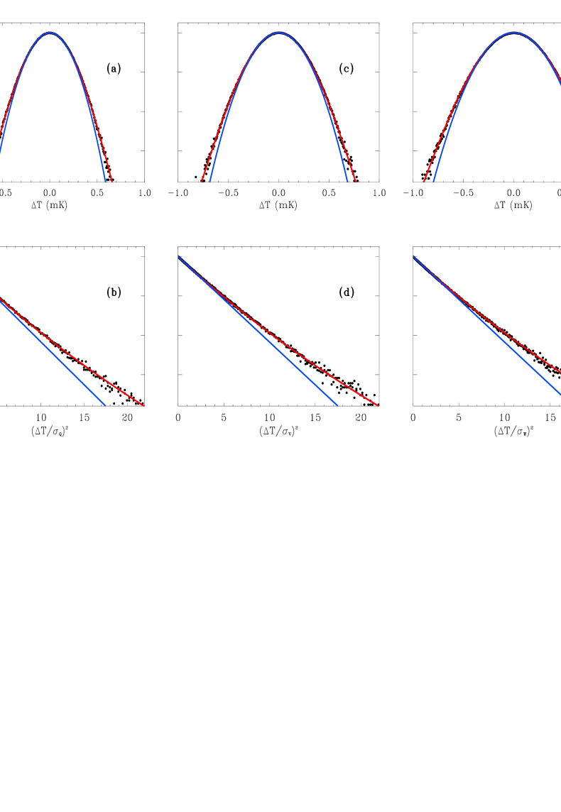
Figure 1: Fits to CMB temperature fluctuations measured by WMAP in bands Q, V, and W (after using the Kp0 mask) applying an exact Gaussian distribution (blue curve) and a nonextensive function (red curve). In figures (a), (c), and (e) we plotted the normalized number of pixels versus $\Delta T$, while in figures (b), (d), and (f) we plotted the normalized number of pixels versus $(\Delta T/\sigma_{\nu})^{2}$, respectively. The $\chi^{2}$ best-fit for the distributions $P_{q}$ gives $q=1.056$, with $\sigma_{{\text{Q}}}=140.58\mu$K, $\sigma_{{\text{V}}}=163.52\mu$K, and $\sigma_{{\text{W}}}=190.35\mu$K, respectively.

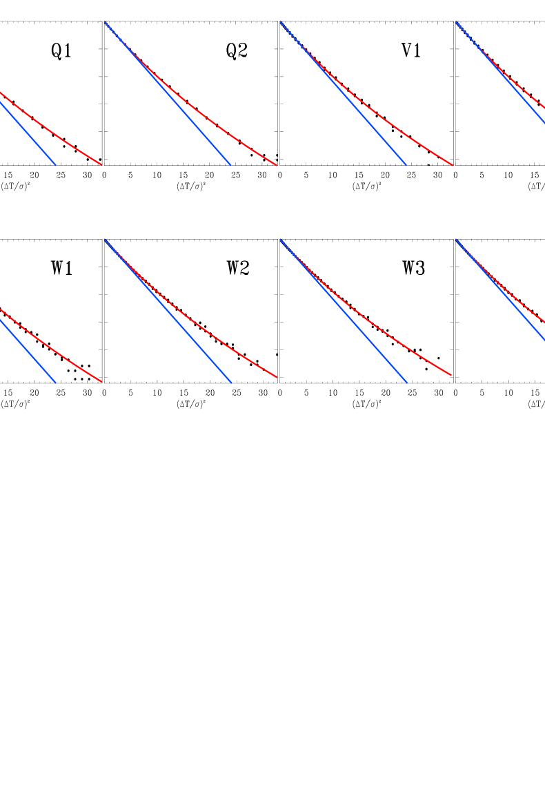
Figure 2: Results of the analysis of WMAP data using the individual radiometer maps Q1, Q2, V1, V2, W1, W2, W3, and W4, after applying the Kp0 mask. In all plots the blue curve represents the best-fit Gaussian, according to the $\chi^{2}$ estimator, while the red curve represents the best nonextensive distribution function. Each $P_{q}$ distributions fits the corresponding data with a slightly different value of $q$, where the mean value of them is $q=1.055\pm 0.002$.

In order to strengthen our analysis, we removed fits to the WMAP foreground templates for the eight individual radiometer maps (corresponding to radiometers Q1, Q2, V1, V2, W1, W2, W3, and W4), after applying the Kp0 mask to avoid high latitude foregrounds. Our results are plotted in Fig. 2. As observed, these results were essentially the same as those shown in Fig. 1, that is, $q=1.055\pm 0.002$.

Then, we investigated the possibility that the discrepancies observed between WMAP data and exact Gaussian distributions, as evidenced in Figs. 1 and 2, occur just by chance. For this scope, we analysed a set of $10,\/000$ Monte Carlo realizations of CMB Gaussian maps, and we found, at the 99% confidence level (CL), that the distributions of CMB temperature fluctuations measured by WMAP are not properly described by exact Gaussian temperature distributions.

We also investigated, through substantial numerical simulations, the possibility that the instrumental noise could introduce non-Gaussian signals in the CMB maps. According to Jarosik et al. (2003); Jeong & Smoot (2005) instrument noise produces a random Gaussian signal, actually Gaussian per observation. Since pixels are observed a different number of times, the effect on the CMB map could be a significant non-Gaussian signal in the CMB temperature distribution, and clearly this possibility should be taken into account in the simulations. For this, to each one of the $10,\/000$ Monte Carlo CMB Gaussian maps we added a simulated non-stationary Gaussian radiometer noise, taking into account the actual number of observations ($n_{i}$) for each pixel in the maps. We consider the $n_{i}$ data from the WMAP-W4 map Bennett et al. (2003). We obtained $q=1.005\pm 0.01$ for the CMB plus non-stationary Gaussian noise simulated maps, which is obviously consistent with Gaussianity. A $\chi^{2}$ estimator test shows that the $P_{q}(\Delta T)$ does not fit the simulated data as well as it does the WMAP data. The monotonic discrepancy behavior observed in Figs. 1b, 1d, and 1f, which is well fitted by the nonextensive expression given in eq. (7) due to a minimum $\chi^{2}$ value, was observed in less than 1% of the simulations performed. Therefore we can rule out, at the 99% CL, the simulated radiometer noise as being the explanation for the non-Gaussianity observed in the WMAP temperature fluctuations.

In conclusion, we have shown that an exact Gaussian distribution is excluded, at the 99% CL, to properly represent the CMB temperature fluctuations measured by WMAP. Although the value of the $q$-parameter is close to 1, our analyses indicate that to consider these temperature fluctuations as being of Gaussian nature is not rigourously exact and it should be considered as a good approximation instead.

We acknowledge use of the Legacy Archive for Microwave Background Data Analysis (LAMBDA). C.T. acknowledges the partial support given by Pronex/MCT, CNPq and FAPERJ (Brazilian Agencies). T.V. acknowledges CNPq grant 302266/88-7-FA and FAPESP grant 00/06770-2. A.B. acknowledges a PCI/DTI/7B-MCT fellowship. We thank Carlos A. Wuensche for his unvaluable help in the Monte Carlo analyses. Some of the results in this paper have been derived using the HEALPix Górski et al. (1998) package.

References

- Fixsen et al. (1996) D. J. Fixsen, et al., Astrophys. J. S. 473, 576 (1996).
- Tsallis et al. (1988) C. Tsallis, J. Stat. Phys. 52, 479 (1988); C. Tsallis, R. S. Mendes, and A. R. Plastino, Physica A 261, 534 (1998).
- Tsallis et al. (1995) C. Tsallis, F. C. Sá Barreto, and E. D. Loh, Phys. Rev. E 52, 1447 (1995); A. R. Plastino, A. Plastino, and H. Vucetich, Phys. Lett. A 207, 42 (1995); M. E. Pessah, D. F. Torres, and H. Vucetich, Physica A 297, 164 (2001).
- Smoot et al. (1992) G. F. Smoot, et al., Astrophys. J. Lett. 396, L1 (1992).
- Ferreira et al. (1998) P. Ferreira, J. Magueijo, and K. Górski, Astrophys. J. 503, 1 (1998).
- Bennett et al. (2003) C. L. Bennett, et al., Astrophys. J. S. 148, 1 (2003).
- Górski et al. (1998) K. M. Górski, E. Hivon, and B. D. Wandelt, astro-ph/9812350.
- Komatsu (2005) E. Komatsu, et al., Astrophys. J. S. 148, 119 (2003); E. Komatsu, D. N. Spergel, and B. D. Wandelt, Astrophys. J. 634, 14 (2005), astro-ph/0305189; H. K. Eriksen, D. I. Novikov, P. B. Lilje, A. J. Banday, and K. M. Gorski, Astrophys. J. 612, 64 (2004), astro-ph/0401276; F. K. Hansen, P. Cabella, D. Marinucci, and N. Vittorio, Astrophys. J. 607, L67 (2004), astro-ph/0402396; K. Land and J. Magueijo, Mon. Not. Roy. Astron. Soc. 357, 994 (2005), astro-ph/0405519; K. Land and J. Magueijo, Mon. Not. Roy. Astron. Soc. 362, L16 (2005), astro-ph/0407081; P. Creminelli, A. Nicolis, L. Senatore, M. Tegmark, and M. Zaldarriaga, astro-ph/0509029; P. D. Naselsky, L.-Y. Chiang, P. Olesen, and I. Novikov, astro-ph/0505011.
- Eriksen et al. (2005) H. K. Eriksen, A. J. Banday, K. M. Gorski, and P. B. Lilje, Astrophys. J. 622, 58 (2005), astro-ph/0407271; T. Wibig and A. W. Wolfendale, Mon. Not. Roy. Astron. Soc. 360, 236 (2005), astro-ph/0409397; P. D. Naselsky, O. V. Verkhodanov, L.-Y. Chiang, and I. Novikov, astro-ph/0310235; astro-ph/0405523.
- Jeong & Smoot (2005) E. Jeong and G. F. Smoot, Astrophys. J. 624, 21 (2005), astro-ph/0406432.
- Copi et al. (2004) C. J. Copi, D. Huterer, and G. D. Starkman, Phys. Rev. D70, 043515 (2004), astro-ph/0310511; L.-Y. Chiang, P. D. Naselsky, O. V. Verkhodanov, and M. J. Way, Astrophys. J. 590, L65 (2003), astro-ph/0303643; P. Vielva, E. Martinez-Gonzalez, R. B. Barreiro, J. L. Sanz, and L. Cayon, Astrophys. J. 609, 22 (2004), astro-ph/0310273; C.-G. Park, Mon. Not. Roy. Astron. Soc. 349, 313 (2004); L.-Y. Chiang, P. D. Naselsky, O. V. Verkhodanov, and M. J. Way, Astrophys. J. 590, L65 (2003), astro-ph/0303643; D. L. Larson and B. D. Wandelt, Astrophys. J. 613, L85 (2004); P. Coles, P. Dineen, J. Earl, and D. Wright, Mon. Not. Roy. Astron. Soc. 350, 983 (2004), astro-ph/0310252; P. D. Naselsky, L.-Y. Chiang, P. Olesen, and O. V. Verkhodanov, Astrophys. J. 615, 45 (2004), astro-ph/0405181; L. Cayon, J. Jin, and A. Treaster, Mon. Not. Roy. Astron. Soc. 362, 826 (2005), astro-ph/0507246; M. Liguori, F. K. Hansen, E. Komatsu, S. Matarrese, and A. Riotto, astro-ph/0509098.
- Copi et al. (2005) C. J. Copi, D. Huterer, D. J. Schwarz, and G. D. Starkman, astro-ph/0508047.
- Anteneodo & Tsallis (1998) C. Anteneodo and C. Tsallis, Phys. Rev. Lett. 80, 5313 (1998); V. Latora, A. Rapisarda, and C. Tsallis, Phys. Rev. E 64, 056134 (2001).
- Gell-Mann & Tsallis (1998) M. Gell-Mann and C. Tsallis, eds., Nonextensive Entropy – Interdisciplinary Applications, (Oxford Univ. Press, New York, 2004); C. Tsallis, J. C. Anjos, and E. P. Borges, Phys. Lett. A 310, 372 (2003); C. Tsallis, S. V. F. Levy, A. M. C. Souza, and R. Maynard, Phys. Rev. Lett. 75, 3589 (1995); Y. S. Weinstein, S. Lloyd, and C. Tsallis, Phys. Rev. Lett. 89, 214101 (2002); M. L. Lyra and C. Tsallis, Phys. Rev. Lett. 80, 53 (1998); C. Beck, Phys. Rev. Lett. 87, 180601 (2001); E. P. Borges, C. Tsallis, G. F. J. Ananos, and P. M. C. de Oliveira, Phys. Rev. Lett. 89, 254103 (2002).
- Tsallis & Bukman (1996) C. Tsallis and D. J. Bukman, Phys. Rev. E 54, R2197 (1996); C. Anteneodo and C. Tsallis, J. Math. Phys. 44, 5194 (2003).
- Jarosik et al. (2003) N. Jarosik, et al., Astrophys. J. S. 148, 29 (2003).
- Bennett et al. (2003) C. L. Bennett, et al., Astrophys. J. S. 148, 97 (2003).