Cosmological Parameter Estimation Using 21 cm Radiation from the Epoch of Reionization

Abstract

A number of radio interferometers are currently being planned or constructed to observe 21 cm emission from reionization. Not only will such measurements provide a detailed view of that epoch, but, since the 21 cm emission also traces the distribution of matter in the Universe, this signal can be used to constrain cosmological parameters at $6\lesssim z\lesssim 20$. The sensitivity of an interferometer to the cosmological information in the signal may depend on how precisely the angular dependence of the 21 cm 3-D power spectrum can be measured. Utilizing an analytic model for reionization, we quantify all the effects that break the spherical symmetry of the 3-D 21 cm power spectrum and produce physically motivated predictions for this power spectrum. We find that upcoming observatories will be sensitive to the 21 cm signal over a wide range of scales, from larger than $100$ to as small as $1$ comoving Mpc. Next, we consider three methods to measure cosmological parameters from the signal: (1) direct fitting of the density power spectrum to the signal (this method can only be applied when density fluctuations dominate the 21 cm fluctuations), (2) using only the velocity field fluctuations in the signal, (3) looking at the signal at large enough scales such that all fluctuations trace the density field. With the foremost method, the first generation of 21 cm observations should moderately improve existing constraints on cosmological parameters for certain low-redshift reionization scenarios, and a two year observation with the second generation interferometer MWA5000 in combination with the CMB telescope Planck can improve constraints on $\Omega_{w}$ (to $\pm 0.017$, a $1.7$ times smaller uncertainty than from Planck alone), $\Omega_{m}\,h^{2}$ ($\pm 0.0009$, $2.5$ times), $\Omega_{b}\,h^{2}$ ($\pm 0.00012$, $1.5$ times), $\Omega_{\nu}$ ($\pm 0.003$, $3$ times), $n_{s}$ ($\pm 0.0033$, $1.4$ times), and $\alpha_{s}$ ($\pm 0.003$, $2.7$ times). Larger interferometers, such as SKA, have the potential to do even better. If the Universe is substantially ionized by $z\sim 12$ or if spin temperature fluctuations are important, we show that it will be difficult to place competitive constraints on cosmological parameters from the 21 cm signal with any of the considered methods.

1. Introduction

The reionization of the Universe involves many poorly understood astrophysical phenomena such as the formation of stars, the escape of ionizing photons from star-forming regions, and the evolving clumpiness of the gas in the intergalactic medium (IGM). However, reionization imprints signatures onto 21 cm emission from high-redshift neutral hydrogen, as will be studied with the instruments PAST, LOFAR, and MWA, in a manner that is sensitive to these processes. Moreover, the 21 cm emission encodes information pertaining to fundamental cosmological parameters. Due to all the overlying astrophysics, it is uncertain whether or not 21 cm observations can be competitive with other cosmological probes.

Several authors have discussed using the 21 cm signal from reionization to study cosmology, in addition to mapping out the epoch of reionization (EOR); (Scott & Rees, 1990; Tozzi et al., 2000; Iliev et al., 2002). Recently, Barkana & Loeb (2005a) show that redshift-space distortions from peculiar velocities allow for the decomposition of the observed 21 cm 3-D power spectrum into terms that are proportional to $\mu^{0},\mu^{2}$ and $\mu^{4}$, where $\mu$ is the cosine of the angle between a mode ${\boldsymbol{k}}$ and the line-of-sight (LOS). In principle, this decomposition makes it possible to separate the contribution from reionized bubbles from that owing to a fundamental cosmological quantity, the linear-theory density power spectrum.

Even if the signal from the ionized bubbles dominates over the cosmological one, Nusser (2005) shows that one can look for an asymmetry between the 21 cm signal measured in depth and that measured in angle. The presence of this asymmetry may imply that the cosmology assumed in the analysis is incorrect [the Alcock-Paczynski (AP) effect]. This effect could help further constrain $\Omega_{m}$ and $h$, as well as dark energy models (Nusser, 2005). It might be possible to distinguish the AP effect because it creates a $\mu^{6}$ dependence in the 3-D power spectrum, which is distinct from the behavior that arises from velocity-field effects alone (Nusser, 2005; Barkana, 2005).

For both the $\mu$ decomposition of the 21 cm power spectrum and the AP effect, the feasibility of inferring cosmological parameters using future surveys depends on how sensitive these surveys are to deviations from spherical symmetry in the 3-D power spectrum. Morales (2005) suggests that 21 cm observations should spherically average ${\boldsymbol{k}}$-modes over a shell in Fourier space to increase the signal-to-noise ratio. In addition to losing the angular information contained in the signal, such averaging would significantly bias upcoming measurements: The power spectrum is not close to spherically symmetric and 21 cm interferometers will be most sensitive to modes oriented along the LOS. Array design also factors into the sensitivity to certain features in the signal. The first generation of EOR arrays are still being planned, and so it is important to understand different design trade-offs.

Authors have considered the 21 cm emission signal in several limits, such as when the spin temperature fluctuations are still important and the HII regions are small (Barkana & Loeb, 2005b; Shapiro et al., 2005) or when the spin temperature is much larger than the cosmic microwave background (CMB) temperature (Zaldarriaga et al., 2004; Furlanetto et al., 2004; Santos et al., 2005). In reality, we do not know how quickly X-rays from the first stars, black holes and shocks will heat the gas and how quickly the spin temperature can couple to the gas temperature via the Wouthuysen-Field effect (Wouthuysen, 1952; Field, 1958). Previous work suggests that these processes act quickly after the first stars turn on (Oh, 2001; Venkatesan et al., 2001; Chen & Miralda-Escudé, 2004; Ciardi & Madau, 2003). Moreover, it is expected that quasars or stellar sources contribute the bulk of the ionizing radiation. If this is the case, reionization will be a patchy process, in which the HII regions grow around these sources as the ionization fraction increases.

Upcoming observations will be most sensitive to lower redshifts ($z\sim 6-12$) during reionization (Bowman et al., 2005a). At these low redshifts, it is likely that the spin temperature is greater than the CMB temperature and that the ionized fraction is of order unity and very patchy. This is the regime that we consider for much of this paper. It is also possible that the ionization fraction is near zero for a period at these low redshifts, which will facilitate cosmological parameter estimation. We consider this case as well.

The organization of this paper is as follows. In §2 we make physically motivated predictions for the form of the 3-D 21 cm power spectrum. We then generalize the detector noise calculation of Morales (2005) to a power spectrum that is not spherically symmetric (§3) and incorporate realistic foregrounds into this sensitivity calculation (§4). These calculations allow us to estimate the sensitivity of upcoming interferometers to the 21 cm power spectrum (§5). We conclude with a discussion of how the 21 cm signal can be used to measure fundamental cosmological parameters as well as a Fisher matrix analysis to estimate how precisely future observations can constrain these parameters (§6).

In our calculations, we assume a cosmology with $\Omega_{m}=0.3$, $\Omega_{\Lambda}=0.7$, $\Omega_{b}=0.046$, $H=100\,h\,{\rm km\;s^{-1}\;{\rm Mpc}^{-1}}$ (with $h=0.7$), $n=1$, and $\sigma_{8}=0.9$, consistent with the most recent determinations (Spergel et al., 2003). All distances are measured in comoving coordinates.

2. Velocity Field Effects

The difference between the observed 21 cm brightness temperature at the observed frequency $\nu$ and the CMB temperature today is (Field, 1959)

$$T_{b}({{\boldsymbol{x}}})=\frac{3c^{2}\,h_{\rm P}\,A_{10}\,n_{H}({{\boldsymbol{x}}})\,a^{3}\,\left[T_{s}({{\boldsymbol{x}}})-T_{\rm CMB}(z)\right]}{32\pi\,k_{B}\,T_{s}({{\boldsymbol{x}}})\,\nu_{0}}\left|\frac{\partial r}{\partial\nu}\right|,$$ (1)

where $c$ is the speed of light, $k_{\rm B}$ is the Boltzmann constant, $h_{\rm P}$ is Planck’s constant, $a=1/(1+z)$, ${\boldsymbol{x}}$ is the spatial location, $T_{\rm CMB}$ is the the CMB temperature, $A_{10}=2.85\times 10^{-15}~{}s^{-1}$ is the spontaneous 21 cm transition rate, $T_{s}$ is the spin temperature, $\nu_{0}=1420\,{\rm MHz}$, and $n_{H}$ is the number density of neutral hydrogen. The factor $|\partial r/\partial\nu|$ accounts for the Hubble flow as well as peculiar velocities. If we take the average of equation (1) we find

$$\bar{T}_{b}\approx 26\,\bar{x}_{H}\left(\frac{\bar{T}_{s}-T_{\rm CMB}}{\bar{T}_{s}}\right)\left(\frac{\Omega_{b}h^{2}}{0.022}\right)\left(\frac{0.15}{\Omega_{m}h^{2}}\,\frac{1+z}{10}\right)^{1/2}~{}{\rm mK}\,,$$ (2)

where $\bar{x}_{H}$ is the global neutral hydrogen fraction. Fluctuations around $\bar{T}_{b}$ are at the tens of mK level on megaparsec scales.

To calculate $\partial r/\partial\nu$, we relate comoving distance to frequency (Bharadwaj & Ali, 2004)

$$r=\int_{\frac{\nu}{\nu_{0}(1-v_{r}/c)}}^{1}\frac{c\,da}{a^{2}\,H(a)},$$ (3)

where $v_{r}$ is the LOS peculiar velocity and $H(a)$ is the Hubble constant. Differentiating this expression, we find

$$\frac{\partial r}{\partial\nu}=-\frac{c}{a^{2}\nu_{0}H}\,\left[1-\frac{1}{Ha}\frac{\partial v_{r}}{\partial r}\right],$$ (4)

where we have dropped terms of order $[(Ha)^{-1}~{}\partial v_{r}/{\partial r}]^{2}$ and $v_{r}/c$. In the limit $T_{s}\gg T_{\rm CMB}$, fluctuations in the 21 cm brightness temperature at ${{\boldsymbol{x}}}$ can be expressed as

$$\frac{\Delta\,T_{b}({{\boldsymbol{x}}})}{\tilde{T}_{b}} = \left(1-\bar{x}_{i}\,[1+\delta_{x}({{\boldsymbol{x}}})]\right)\,\left(1+\delta({{\boldsymbol{x}}})\right)$$ (5)

$$\times \left(1-\frac{1}{Ha}\frac{\partial v_{r}({{\boldsymbol{x}}})}{\partial r}\right)-\bar{x}_{H},$$

where $\bar{x}_{i}\equiv 1-\bar{x}_{H}$ is the global ionized fraction, $\delta_{x}$ is the overdensity in the ionized fraction and $\delta$ is the dark matter overdensity (at the scales and redshifts of interest, the baryons trace the dark matter). We define the normalized temperature as $\tilde{T}_{b}\equiv\bar{T}_{b}/\bar{x}_{H}$. In Fourier space, since the linear theory velocity at redshifts where dark energy is unimportant is $v(k,z)=-{\it i}\,H\,a\,{{\boldsymbol{k}}}\,\delta_{L}/k^{2}$, the peculiar velocity term is $\delta_{v}\equiv(Ha)^{-1}~{}\partial v_{r}/\partial r=-\mu^{2}\delta_{L}$ where $\mu\equiv\hat{{{\boldsymbol{k}}}}\cdot\hat{{\bf n}}$, the cosine of the angle between the wavevector and the LOS, and $L$ denotes the linear theory value. If we keep terms to second order in $\{\delta,\delta^{L}\}$, the brightness temperature power spectrum is

$$\tilde{T}_{b}^{-2}~{}P_{\Delta T}({{\boldsymbol{k}}}) = \left[\bar{x}_{H}^{2}\,P_{\delta\delta}+P_{xx}-2\bar{x}_{H}\,P_{x\delta}+P_{x\delta x\delta}\right]$$ (6)

$$+ 2\mu^{2}\left[\bar{x}_{H}^{2}\,P_{\delta_{L}\delta}-\bar{x}_{H}\,P_{x\delta_{L}}\right]+\mu^{4}\left[\bar{x}_{H}^{2}\,P_{\delta_{L}\delta_{L}}\right]$$

$$+ \left[2P_{x\,\delta\,\delta_{v}x}+P_{x\,\delta_{v}\,\delta_{v}\,x}\right],$$

and we note that $P_{xx}=\bar{x}_{i}^{2}\,P_{\delta_{x}\delta_{x}}$ and $P_{x\delta}=\bar{x}_{i}\,P_{\delta_{x}\delta}$. In our calculations, we drop the connected part and set $P_{x\delta x\delta}=P_{x\delta}^{2}+P_{xx}\,P_{\delta\delta}$. In equation 6, we have decomposed the power spectrum into powers of $\mu$; the last bracket in this decomposition has a non-trivial dependence on $\mu$. For notational convenience, we refer to the k-dependent coefficients in equation (6) as $P_{\mu^{0}}$, $P_{\mu^{2}}$ and $P_{\mu^{4}}$ and the terms in the last bracket as $P_{f(\mu,k)}$. Barkana & Loeb (2005a) argue that the above decomposition should allow one to extract the “physics” – ($P_{\delta_{L}\delta_{L}}$)– from the “astrophysics”– ($P_{xx}$ and $P_{x\delta}$). The terms in the last bracket in equation (6) were omitted in their analysis, but must be included if reionization is patchy because $\delta_{x}\sim 1$ on scales at or below the bubble size. If we drop the connected fourth moments, the $P_{f(\mu,k)}$ terms are given by

$$P_{x\,\delta\,\delta_{v}\,x}({{\boldsymbol{k}}}) = \int\frac{d^{3}{{\boldsymbol{k}}^{\prime}}}{(2\pi)^{3}}({\hat{\boldsymbol{n}}}\cdot{\hat{{\boldsymbol{k}}^{\prime}}})^{2}\,[P_{x\delta_{L}}(k^{\prime})~{}P_{x\delta}(|{{\boldsymbol{k}}-{\boldsymbol{k}}^{\prime}}|)$$

$$+ P_{\delta_{L}\delta}(k^{\prime})~{}P_{xx}(|{{\boldsymbol{k}}-{\boldsymbol{k}}^{\prime}}|)],$$

$$P_{x\,\delta_{v}\,\delta_{v}\,x}({{\boldsymbol{k}}}) = \int\frac{d^{3}{{\boldsymbol{k}}^{\prime}}}{(2\pi)^{3}}[({\hat{\boldsymbol{n}}}\cdot{\hat{{\boldsymbol{k}}^{\prime}}})^{4}\,P_{\delta_{L}\delta_{L}}(k^{\prime})~{}P_{xx}(|{{\boldsymbol{k}}-{\boldsymbol{k}}^{\prime}}|)$$ (7)

$$+ ({\hat{\boldsymbol{n}}}\cdot{\hat{{\boldsymbol{k}}^{\prime}}})^{2}~{}\left({\hat{\boldsymbol{n}}}\cdot\left[\frac{{\boldsymbol{k}}-{\boldsymbol{k}}^{\prime}}{|{{\boldsymbol{k}}-{\boldsymbol{k}}^{\prime}}|}\right]\right)^{2}$$

$$\times P_{x\delta_{L}}(k^{\prime})~{}P_{x\delta_{L}}(|{{\boldsymbol{k}}-{\boldsymbol{k}}^{\prime}}|)],$$

where $k^{\prime}=({\boldsymbol{k}}^{\prime}\cdot{\boldsymbol{k}}^{\prime})^{1/2}$. These terms can contaminate the $\mu$ decomposition. On large scales, $P_{f(\mu,k)}$ does not depend on $\mu$ and therefore will contaminate only measurements of $P_{\mu^{0}}$. As we go to progressively smaller scales, $P_{f(\mu,k)}$ contributes power to higher order terms in $\mu$.

The evolution of the ionized fraction over a mode can also affect the spherical symmetry of $P_{\Delta T}$, since time is changing in the LOS direction but not in the angular directions. The magnitude of this effect depends strongly on the morphology of reionization and is discussed in Appendix A.

2.1. Model

To model reionizaton by stellar sources, simulations must resolve halos at least as small as the HI cooling mass ($\sim 10^{8}~{}M_{\odot}$) as well as have boxes large enough to sample the size distribution of HII regions, which can each reach larger scales than $10~{}{\rm Mpc}$ (Furlanetto et al., 2004; Barkana & Loeb, 2005b). Recent simulations have made significant strides towards attaining these goals (Iliev et al., 2005; Kohler et al., 2005). For the time being, semi-analytic models of this epoch provide a convenient approach for modeling reionization on the large scales that are relevant for upcoming observations. In this paper, we employ the physically motivated semi-analytic model described in Furlanetto et al. (2004a; hereafter FZH04) to calculate $P_{\Delta T}$.

Recent numerical simulations (e.g., Sokasian et al. 2003, 2004; Ciardi et al. 2003) show that reionization proceeds “inside-out” from high density clusters of sources to voids, at least when the sources resemble star-forming galaxies (e.g., Springel & Hernquist 2003; Hernquist & Springel 2003). We therefore associate HII regions with large-scale overdensities. We assume that a galaxy of mass $m_{\rm gal}$ can ionize a mass $\zeta m_{\rm gal}$, where $\zeta$ is a constant that depends on: the efficiency of ionizing photon production, the escape fraction, the star formation efficiency, and the number of recombinations. Values of $\zeta\lesssim 10-40$ are reasonable for normal star formation, but very massive stars can increase the efficiency by an order of magnitude (Bromm et al., 2001).

The criterion for a region to be ionized by the galaxies contained inside it is then $f_{\rm coll}>\zeta^{-1}$, where $f_{\rm coll}$ is the fraction of mass bound to halos above some minimum mass $m_{\rm min}$. We assume that this minimum mass corresponds to a virial temperature of $10^{4}{\rm K}$, at which point hydrogen line cooling becomes efficient. The function $f_{\rm coll}$ depends on the assumed halo mass function. Furlanetto et al. (2005) find that the choice of the mass function has an insignificant effect on the FZH04 model. Here we use the Press-Schechter mass function. In the extended Press-Schechter model (Bond et al., 1991; Lacey & Cole, 1993) the collapse fraction of halos above the critical mass $m_{\rm min}$ in a region of mean overdensity $\delta_{m}$ is

$$f_{\rm coll}={\rm erfc}\left(\frac{\delta_{c}-\delta_{m}}{\sqrt{2\left[\,\sigma^{2}_{\rm min}-\sigma^{2}(m,z)\right]}}\right),$$ (8)

where $\sigma^{2}(m,z)$ is the variance of density fluctuations on the scale $m$, $\sigma^{2}_{\rm min}\equiv\sigma^{2}(m_{\rm min},z)$ and $\delta_{c}\approx 1.686$, the critical density for collapse. With this equation for the collapse fraction, we can write a condition on the mean overdensity within an ionized region of mass $m$,

$$\delta_{m}\geq\delta_{B}(m,z)\equiv\delta_{c}-\sqrt{2}K(\zeta)[\sigma^{2}_{\rm min}-\sigma^{2}(m,z)]^{1/2},$$ (9)

where $K(\zeta)={\rm erf}^{-1}\left(1-\zeta^{-1}\right)$.

FZH04 showed how to construct the mass function of HII regions from $\delta_{B}$ in a manner analogous to that of the halo mass function (Press & Schechter, 1974; Bond et al., 1991). The barrier in equation (9) is well approximated by a linear function in $\sigma^{2}$, $\delta_{B}\approx B(m)=B_{0}+B_{1}\sigma^{2}(m)$, where the redshift dependence is implicit. In that case, the mass function has an analytic expression (Sheth, 1998):

$$n(m)=\sqrt{\frac{2}{\pi}}\ \frac{\bar{\rho}}{m^{2}}\ \left|\frac{d\ln\sigma}{d\ln m}\right|\ \frac{B_{0}}{\sigma(m)}\exp\left[-\frac{B^{2}(m)}{2\sigma^{2}(m)}\right],$$ (10)

where $\bar{\rho}$ is the mean density of the Universe. Equation (10) gives the comoving number density of HII regions with masses in the range $(m,m+dm)$. The crucial difference between this formula and the standard Press-Schechter mass function occurs because $\delta_{B}$ is a decreasing function of $m$. The barrier becomes more difficult to cross on smaller scales, which gives the bubbles a characteristic size.

We can calculate $P_{xx}$ and $P_{x\delta}$ for the FZH04 model with the semi-analytic method described in McQuinn et al. (2005). It is more difficult to calculate $P_{x\delta_{L}}$. McQuinn et al. (2005) showed that it is not necessary to consider bubble substructure in this analytic model when constructing $P_{x\delta}$; – only the size of a bubble and the average density within a bubble are important. Since we can ignore bubble substructure, this implies that $P_{x\delta}\rightarrow P_{x\delta_{L}}$ when the effective HII bubble radius reaches linear scales. This happens in the FZH04 model when $\bar{x}_{i}\gtrsim 0.25$. In the opposite limit, when the bubbles are very small, this term is subdominant to density fluctuations and so has a small effect on the power spectrum. We set $P_{x\delta_{L}}=P_{x\delta}$ for all times. This will result in an overestimate of this term when $\bar{x}_{i}$ is small and therefore an underestimate of $P_{\mu^{2}}$.

For our calculations in this section, our objective is not to model the 21 cm power spectrum for different reionization scenarios and discuss morphological differences. In the context of the FZH04 model, this has been done in FZH04, Furlanetto et al. (2004b), and Furlanetto et al. (2005). Instead, we restrict ourselves to one parameterization of this model, setting $\zeta(z)=12$, in order to illustrate the effect of redshift-space distortions on $P_{\Delta T}$. For this parameterization, the EOR spans roughly the redshifts $8-15$. In reality, $\zeta$ will have some time dependence, and it may even have a very complicated evolution. Fortunately, we find that the parameterization $\zeta=12$ is representative of the FZH04 model: while varying the function $\zeta(z)$ will change $\bar{x}_{i}(z)$, if we identify the same ionization fraction for different values of $\zeta$, the values of $P_{xx}$ are quite similar (FZH04).

Of course, reionization might proceed differently than in this analytic model. The parameter $\zeta$ may depend on the mass of the dark matter halo. This can have a modest effect on the characteristic size of the bubbles and the large-scale bubble bias (Furlanetto et al., 2005). Also, recombinations might play a larger role in shaping the morphology of reionization. Employing reasonable assumptions for the clumpiness of the IGM, Furlanetto & Oh (2005) show that the effect of recombinations in the FZH04 model is only important at $\bar{x}_{i}\gtrsim 0.7$, increasing in importance as $\bar{x}_{i}\rightarrow 1$. The presence of mini-halos may make recombinations more important (Shapiro et al., 2003), but recent work suggests that this may not be the case (Ciardi et al., 2005). So long as recombinations are not important, Furlanetto et al. (2005) showed that any model where the ionizing sources trace the collapsed regions must have a qualitatively similar bubble size distribution to the FZH04 distribution.

Figure 1 plots for $\zeta=12$ the components of the dimensionless power spectrum, $k^{3}\,P_{\Delta T}/2\pi^{2}$, that have different $\mu$ dependences. The thick solid, thick dashed and thick dot-dashed curves indicate the $P_{\mu^{0}}$, $P_{\mu^{2}}$, and $P_{\mu^{4}}$ terms, respectively. The $\mu$ dependence of $P_{f(\mu,k)}$ is nontrivial. The three thin solid curves indicate the total contribution from $P_{f(\mu,k)}$ for $\mu^{2}=0.0,0.5$ and $1.0$ (in order of increasing amplitude).

At $\bar{x}_{i}=0.1$, $P_{\mu^{4}}$ is the largest of the $\mu$-terms (see Fig. 1, right). This is because the neutral regions are underdense on average, and, at small $\bar{x}_{i}$, this results in a suppression of $P_{\mu^{0}}$ and $P_{\mu^{2}}$. The $\mu$ decomposition of the signal can be much different at larger ionization fractions. For $\bar{x}_{i}=0.7$, $P_{\mu^{0}}$ is much larger than the other terms at most scales (see Fig.1, left), and $P_{\mu^{2}}$ becomes negative at small $k$ because the neutral gas is underdense on average. Finally, at smaller scales than the bubbles size, $P_{f(\mu,k)}$ is larger than $P_{\mu^{2}}$ and $P_{\mu^{4}}$, and is even larger than $P_{\mu^{0}}$ at $k\approx 3\,{\rm Mpc}^{-1}$.

The evolution of the spherical symmetry as a function of $\bar{x}_{i}$ is non-trivial. When the ionization fraction is small, the redshift space distortions are important on all scales. In the opposite limit, when the ionization fraction is large, the redshift-space effects are less important since the bubble-bubble term $P_{xx}$, which enters through $P_{\mu^{0}}$, dominates the signal (Fig. 1, left). The evolution of the angular symmetry of the signal is illustrated in Figure 2, which plots the contours of constant $k^{3}\,P_{\Delta T}(k)$ for $\bar{x}_{i}=0.1$ and $\bar{x}_{i}=0.7$ (right and left panels, respectively). When $\bar{x}_{i}=0.7$, the signal is fairly symmetric at smaller $k$-modes than the bubble scale. At larger values of $k$ or at small ionization fractions, density fluctuations dominate the signal, and the power spectrum can be very asymmetric. Because of this, it may be possible to determine the characteristic bubble size by observing the angular dependence of $P_{\Delta T}$.

In Figure 3, we plot the signal $[k^{3}\,P_{\Delta T}(k,\mu)/2\pi^{2}]$ for modes with $\mu^{2}=0.0,0.5,~{}{\rm and}~{}1.0$ (the solid, dot-dashed, and dashed curves, respectively) at four times during reionization. Between $\bar{x}_{i}\sim 0.0-0.1$, density fluctuations dominate the signal and the signal is very asymmetric. By $\bar{x}_{i}=0.5$, the neutral fraction fluctuations contribute most of the power on large scales. When these fluctuation dominate, the 21 cm power spectrum develops a “shoulder” on scales near the characteristic bubble size. This feature moves to larger scales as the bubbles grow.

In §5, we show that upcoming interferometers will be more sensitive to modes with certain orientations relative to the LOS. It turns out that arrays that are very compact (i.e. have most of their antennae within a 1 km region), such as MWA, are most sensitive to $k$-modes that are oriented along the LOS. The fact that these modes have more power enhances MWA’s sensitivity. Conversely, it is difficult to separate the terms $P_{\mu^{0}}$, $P_{\mu^{2}}$ and $P_{\mu^{4}}$ with observations that are most sensitive to the modes along the LOS.

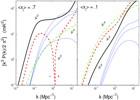
Figure 1.— The $\mu$ decomposition of the signal (see equation 6) for $\bar{x}_{i}=0.1$ and $0.7$, corresponding to $z=13.5$ and $9$ in the $\zeta=12$ model. The thick solid, thick dashed and thick dot-dashed curves show $P_{\mu^{0}}$, $P_{\mu^{2}}$, and $P_{\mu^{4}}$, respectively. The three thin solid curves show $P_{f(\mu,k)}$, calculated using equation (7) with $\mu^{2}=0.0,0.5$ and $1.0$ (in order of increasing amplitude).

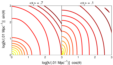
Figure 2.— Contours of constant $k^{3}P_{\Delta T}(k)$ for the same signal as in Figure 1. The horizontal axis is the LOS direction, and the vertical axis is the transverse direction. The coordinate transformation $(k_{\perp},k_{||})\rightarrow\log(k/(0.01~{}{\rm Mpc}^{-1}))(\sin(\theta),\cos(\theta))$ preserves circles of constant power.

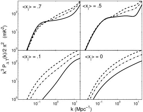
Figure 3.— Dimensionless power spectrum $k^{3}\,P_{\Delta T}/2\pi^{2}$ for $\mu^{2}$ equal to $0.0,\,0.5,$ and $1.0$ (solid, dash-dot, and dashed lines, respectively) for four times during reionization in the $\zeta=12$ model, corresponding to $z=$ 9, 9.8, 13.5 and 20 (in order of decreasing $\bar{x}_{i}$). The signal is most asymmetric at scales where density fluctuations dominate.

3. Sensitivity to the 21 cm Power Spectrum

In this section, we summarize how to calculate the variance on interferometric observations of the 3-D 21 cm power spectrum. Our calculation follows that of Morales (2005), and extends their calculation to capture the angular dependence of the 3-D signal. White et al. (1999) and Zaldarriaga et al. (2004) do a similar interferometric detector noise calculation, but for the angular power spectrum. For 21 cm observations, the 3-D power spectrum is more interesting than the angular power spectrum owing in part to the the $\mu$ dependence of the signal. In addition, the 3-D power spectrum will allow us to measure many more independent modes.

The 21 cm signal will be observed with radio interferometers, which measure visibilities. The visibility for a pair of antennae, quantified as a temperature, is given by

$$V(u,v,\nu)=\int{d{{\hat{\boldsymbol{n}}}}\,\,\Delta T_{b}({\hat{\boldsymbol{n}}},\nu)\,A_{\nu}({\hat{\boldsymbol{n}}})e^{2\pi{\it i}{u\choose v}\cdot{\hat{\boldsymbol{n}}}}},$$ (11)

where $(u,v)$ is a vector that gives the number of wavelengths at frequency $\nu$ between the antennae and $A_{\nu}({\hat{\boldsymbol{n}}})$ is the contribution to the primary beam in the direction ${\hat{\boldsymbol{n}}}$. Here, we are working in the flat sky approximation; this is adequate since upcoming experiments are most sensitive to angular modes with wavelength $\theta<0.1$ radians.

We assume that the visibilities are complex Gaussian random variables, such that the likelihood function of the covariance matrix $C_{i\,j}=\langle{V}^{*}_{i}\,{V}_{j}\rangle$ for $n$ visibilities, where the asterisk indicates a complex conjugate, is

$${\cal L}({\boldsymbol{C}})=\frac{1}{\pi^{n}\,{\rm det}{\boldsymbol{C}}}~{}\exp\left[-\mathop{\sum}_{i,j}^{n}{\,{V}_{i}^{*}\,C_{ij}^{-1}\,{V}_{j}}\right].$$ (12)

Because the visibilities are complex and ${V}(u,v,\nu)={V}(-u,-v,\nu)^{*}$, when counting the number of independent $u$-$v$ pixels we restrict ourselves to the half space. In this section, it will be more convenient to work with the Fourier transform of $\boldsymbol{V}$ in the frequency direction. This is just a change of basis of $\boldsymbol{V}$ and $\boldsymbol{C}$ in equation (12).

For upcoming arrays, $\boldsymbol{C}$ will be dominated by the detector noise on most scales. The RMS detector noise fluctuation per visibility of an antennae pair after observing for a time $t_{0}$ in one frequency channel is (Rohlfs & Wilson, 2004)

$$\Delta V^{N}=\frac{\lambda^{2}T_{\rm sys}}{A_{e}\,\sqrt{\Delta\nu\,t_{0}}},$$ (13)

where $T_{\rm sys}(\nu)$ is the total system temperature, $A_{e}$ is the effective area of an antenna, and $\Delta\nu$ is the width of the frequency channel.

For an observation with bandwidth $B$, where $B\gg\Delta\nu$, if we Fourier transform the observed visibilities in the frequency direction, we then have a 3-D map of $\tilde{I}({\boldsymbol{u}})\equiv\int d\nu{V}(u,v,\nu)\exp[2\pi i\nu\eta]$, in which ${\boldsymbol{u}}=u\,\hat{\boldsymbol{i}}+v\,\hat{\boldsymbol{j}}+\eta\,\hat{\boldsymbol{k}}$ and $\eta$ has dimensions of time. If we perform this transform on just the detector noise component $\boldsymbol{V}^{N}$ of the visibility map $\boldsymbol{V}$, we have

$$\tilde{I}^{N}({\boldsymbol{u}}) = \mathop{\sum}_{i=1}^{B/\Delta\nu}\,{V}^{N}(u,v,\nu_{i})\,\exp[2\pi i\nu_{i}\eta]\,\Delta\nu$$ (14)

$$= \mathop{\sum}_{i=1}^{B/\Delta\nu}\,{V^{\prime}}^{N}(u,v,\nu_{i})\,\Delta\nu,$$ (15)

where we have absorbed $\exp[2\pi i\nu\eta]$ into a new variable $V^{\prime N}$ that has the same RMS as ${V}^{N}$ and the frequency channels $\nu_{1},...,\nu_{B/\Delta\nu}$ are spaced $\Delta\nu$ apart. It follows that the detector noise covariance matrix for a single baseline is (Morales, 2005)

$$C^{N}_{1b}({\boldsymbol{u}}_{i},{\boldsymbol{u}}_{j}) = \langle\tilde{I}^{N}({\boldsymbol{u}}_{i})^{*}\,\tilde{I}^{N}({\boldsymbol{u}}_{j})\rangle$$ (16)

$$= \langle\left(\mathop{\sum}_{m=1}^{B/\Delta\nu}\,{V^{\prime}}^{N}({\boldsymbol{u}}_{i},\nu_{m})\,\Delta\nu\right)^{*}$$

$$\times\left(\mathop{\sum}_{l=1}^{B/\Delta\nu}\,{V^{\prime}}^{N}({\boldsymbol{u}}_{j},\nu_{l})\,\Delta\nu\right)\rangle$$

$$= B\,\Delta\nu\,\left(\Delta V^{N}\right)^{2}\,\delta_{ij}$$

$$= \left(\frac{\lambda^{2}\,B\,T_{\rm sys}}{A_{e}}\right)^{2}\,\frac{\delta_{ij}}{B\,t_{0}}.$$ (17)

To reach equation (16), we note that different ${V}^{\prime N}({\boldsymbol{u}}_{i},\nu_{m})$ are uncorrelated, and equation (17) follows from equations (13) and (16). Note that equation (17) only depends on $B$ and not on $\Delta\nu$: finer frequency resolution comes at no added cost.

We now estimate the average observing time $t_{\boldsymbol{k}}$ for an array of antennae to observe a mode ${\boldsymbol{k}}$ as a function of the total observing time $t_{0}$ (note that there is an isomorphism ${\boldsymbol{u}}\leftrightarrow{\boldsymbol{k}}$ and that $2\pi{\boldsymbol{u}}_{\perp}/x={\boldsymbol{k}}_{\perp}$, where x is the conformal distance to the emission). At any time, the number density of baselines that can observe the mode ${\boldsymbol{u}}$ is $n({\boldsymbol{u}}_{\perp})$. We assume this density is rotationally invariant and define $\theta$ to be the angle between ${\boldsymbol{k}}$ and the LOS. Integrating $n({\boldsymbol{u}}_{\perp})\,du\,dv$ over the half plane yields $N_{\rm base}\approx N_{\rm ant}^{2}/2$, where $N_{\rm ant}$ is the number of antennae. Since the telescope observes a region in the $u$-$v$ plane equal to $\delta u\delta v\approx A_{e}/\lambda^{2}$, each visibility is observed for a time

$$t_{\boldsymbol{k}}\approx\frac{A_{e}\,t_{0}}{\lambda^{2}}\,n(x\,|{\boldsymbol{k}}|\,{\rm sin}(\theta)/2\pi),$$ (18)

where $t_{0}$ is the total observing time for the interferometer. It follows that the detector noise covariance matrix for an interferometer is

$$C^{N}({\boldsymbol{k}}_{i},{\boldsymbol{k}}_{j})=\left(\frac{\lambda^{2}\,B\,T_{\rm sys}}{A_{e}}\right)^{2}\,\frac{\delta_{ij}}{B\,t_{{\boldsymbol{k}}_{i}}}.$$ (19)

(From now on we will use ${\boldsymbol{k}}$ rather than ${\boldsymbol{u}}$ to index elements in $\boldsymbol{C}$).

We also want an expression for the contribution to $\boldsymbol{C}$ owing to sample variance. For a 3-D window function ${W}({\hat{\boldsymbol{n}}},\nu)=A_{\nu}({\hat{\boldsymbol{n}}})~{}F_{\hat{\boldsymbol{n}}}(\nu)$, if we assume that different pixels indexed by ${\boldsymbol{u}}$ are uncorrelated, the covariance matrix of the 21 cm signal $\tilde{I}^{21}$ is

$$C^{SV}({\boldsymbol{k}}_{i},{\boldsymbol{k}}_{j}) = \langle\tilde{I}^{21}({\boldsymbol{u}}_{i})^{*}\tilde{I}^{21}({\boldsymbol{u}}_{j})\rangle$$ (20)

$$\approx ~{}\delta_{ij}~{}\int d^{3}{\boldsymbol{u}}^{\prime}\,|\tilde{W}({\boldsymbol{u}}_{i}-{\boldsymbol{u}}^{\prime})|^{2}\,P^{21}_{\Delta T}({\boldsymbol{u}}^{\prime}),$$

where we have used that $\langle\Delta T^{21}({\boldsymbol{u}}^{\prime})\Delta\,T^{21}({\boldsymbol{u}})\rangle=P_{\Delta T}({\boldsymbol{u}})~{}\delta^{3}({\boldsymbol{u}}^{\prime}-{\boldsymbol{u}})$ and the definition of visibility (eqn. 11). We can simplify $\boldsymbol{C}^{SV}$ further:

$$C^{SV}({\boldsymbol{k}}_{i},{\boldsymbol{k}}_{j}) \approx ~{}P^{\rm 21}_{\Delta T}({\boldsymbol{u}}_{i})\,\frac{\lambda^{2}\,B}{A_{e}}~{}\delta_{ij}$$ (21)

$$\approx ~{}P^{21}_{\Delta T}({\boldsymbol{k}}_{i})\,\frac{\lambda^{2}\,B^{2}}{A_{e}\,x^{2}\,y}~{}\delta_{ij},$$ (22)

where to get to equation (21) we pull $P({\boldsymbol{u}}_{i})$ out of the integral and use the fact that $\tilde{W}({\boldsymbol{u}})$ is different from zero in an area $\delta u\delta v\delta\eta\approx A_{e}/(\lambda^{2}\,B)$ and must integrate to unity within the beam, such that $\int d^{3}{\boldsymbol{u}}^{\prime}\,|\tilde{W}({\boldsymbol{u}}-{\boldsymbol{u}}^{\prime})|^{2}\approx(\delta u\delta v\delta\eta)^{-1}$. Equation (21) is accurate for values of $|{\boldsymbol{u}}_{i}|$ much greater than the FWHM of $\tilde{W}$. The additional factor of $x^{2}y/B$ that arises in equation (22) is because with our Fourier conventions $P_{\Delta T}({\boldsymbol{k}})=x^{2}y/B\,P_{\Delta T}({\boldsymbol{u}})$, where $y$ is the conformal width of the observation.

Over the course of an observation, a large number of independent Fourier cells will be observed in a region of real space volume ${\rm Vol}=x^{2}\,y\,\lambda^{2}/A_{e}$. We have seen that the 21 cm power spectrum is not spherically symmetric, but is symmetric around the polar angle $\phi$. Because of this symmetry, we want to sum all the Fourier cells in an annulus of constant $(k,\theta)$ with radial width $\Delta k$ and angular width $\Delta\theta$ for a statistical detection. The number of independent cells in such an annulus is

$$N_{c}(k,\theta)=2\pi{k}^{2}\,\sin(\theta)\,\Delta k\,\Delta\theta\times\frac{\rm Vol}{(2\pi)^{3}}.$$ (23)

Here, $(2\pi)^{3}/{\rm Vol}$ is the resolution in Fourier space. For our calculations, we use equation (23) for $N_{c}$ when the wavelength corresponding to ${\boldsymbol{k}}$ fits within the survey volume (i.e. when $2\pi/k\,\cos(\theta)<y$) and otherwise we set $N_{c}=0$.

When we sum equations (19) and (22) to get $\boldsymbol{C}$, the error in $P^{21}_{\Delta T}({\boldsymbol{k}})$ from a measurement in an annulus with $N_{c}(k,\theta)$ pixels is

$$\delta P^{21}_{\Delta T}(k,\theta)\approx\sqrt{\frac{1}{N_{c}}}\,\frac{A_{e}\,x^{2}\,y}{\lambda^{2}\,B^{2}}\,\left[{\rm C}^{SV}(k,\theta)+{\rm C}^{N}(k,\theta)\right],$$ (24)

where we have defined ${\rm C}({\boldsymbol{k}})\equiv C({\boldsymbol{k}},{\boldsymbol{k}})$. One can trivially derive equation (24) by calculating the Fisher matrix $\boldsymbol{F}$ of the $P({\boldsymbol{k}}_{i})$ from $\boldsymbol{C}$ (e.g. eqn. 31, with $\tilde{{\boldsymbol{C}}}\rightarrow\boldsymbol{C}$), noting that there are $N_{c}$ measurements of $P(k,\theta)$ and that $\delta P^{21}_{\Delta T}({\boldsymbol{k}})=\sqrt{{F^{-1}}_{{\boldsymbol{k}}{\boldsymbol{k}}}}$.

Given a model for the data, the 1-$\sigma$ errors in the model parameters $\lambda_{i}$ are ($\sqrt{{F^{\prime-1}}_{ii}}$), where

$$F^{\prime}_{ij}=\sum_{\rm pixels}\frac{1}{(\delta P_{\Delta T})^{2}}\,\frac{\partial P_{\Delta T}}{\partial\lambda_{i}}\,\frac{\partial P_{\Delta T}}{\partial\lambda_{j}}.$$ (25)

[See Appendix B for a useful formula for $\delta P_{\Delta T}(k)$, the error in the angular-averaged power spectrum.]

In the next section, we extend the above analysis to include foregrounds. The calculation in this section assumes Gaussian statistics, but the ionization fraction fluctuations on the scale of the HII bubbles will not be Gaussian. Numerical simulations are necessary to quantify the degree of non-Gaussianity introduced by patchy reionization.

4. Foregrounds

The foregrounds at $\lambda=21\,(1+z)$ cm will be at temperatures of hundreds to thousands of kelvin, approximately $4$ orders of magnitude greater than the 21 cm signal. All the significant foreground contaminants should have smooth power-law spectra. Known sources of radio recombination lines are estimated to contribute to the fluctuations at an insignificant level (Oh & Mack, 2003).

Before fitting a model to the cosmological signal, it is necessary to clean the foregrounds from the data. The idea is to subtract out a smooth function from the total signal prior to the parameter fitting stage (Tegmark et al., 2000). Such pre-processing is common with CMB data sets, and Wang et al. (2005) showed that this procedure can also be used in handling 21 cm observations.

At the frequency $\nu_{i}$ in a pixel with angular index ${\boldsymbol{k}}_{\perp}$, an interferometer measures

$$x_{i}=s({\boldsymbol{k}}_{\perp},\nu_{i})+n({\boldsymbol{k}}_{\perp},\nu_{i})+f({\boldsymbol{k}}_{\perp},\nu_{i}),$$ (26)

where $s$ is the 21 cm signal in visibilities, $n$ is the detector noise fluctuation, and $f$ is the foreground amplitude (all of which are complex). We will subsequently write the quantities $x,s,n$ and $f$ measured at the N frequencies ${\mbox{\boldmath$\nu$}}=(\nu_{1},...,\nu_{N})$ with resolution $\Delta\nu$ as the vectors ${{\boldsymbol{x}}},{{\boldsymbol{s}}},{{\boldsymbol{n}}}$, and ${{\boldsymbol{f}}}$. There is one key difference between our calculation and that of Wang et al. (2005). Rather than subtracting from $\log({x})$ a polynomial in $\log({\nu})$, which is functionally very similar to the known foregrounds, we instead subtract a polynomial in ${\nu}$ from $x$. While this difference may require a higher order function to adequately fit the data, it also permits an analytic treatment.

Fitting an order-${\rm n}$ polynomial to the vector ${\boldsymbol{x}}$ is equivalent to projecting out the Legendre polynomials ${{\boldsymbol{P}}}_{0},{{\boldsymbol{P}}}_{1},...,{{\boldsymbol{P}}}_{\rm n}$, normalized such that $\int_{0}^{B}P_{l_{1}}(2\nu/B-1)P_{l_{2}}(2\nu/B-1)d\nu=\delta_{l_{1},l_{2}}$ and ${P_{l,\,i}}=P_{l}(2\nu_{i}/B-1)\,\sqrt{\Delta\nu}$. Projecting out to order n, our cleaned signal is

$$\tilde{{\boldsymbol{x}}}=\left(1-\sum_{l=0}^{\rm n}\,{{\boldsymbol{P}}}_{l}\,{{\boldsymbol{P}}}_{l}^{T}\right)\,{\boldsymbol{x}}~{}\equiv~{}\sum_{l={\rm n}+1}^{N}\,{{\boldsymbol{P}}}_{l}\,{{\boldsymbol{P}}}_{l}^{T}\,{\boldsymbol{x}}.$$ (27)

and $\tilde{{\boldsymbol{s}}}$, $\tilde{{\boldsymbol{n}}}$ and $\tilde{{\boldsymbol{f}}}$ are defined in analogy to $\tilde{{\boldsymbol{x}}}$. The covariance matrix for the cleaned signal is $\tilde{{\boldsymbol{C}}}\equiv\langle\tilde{{\boldsymbol{x}}}\,\tilde{{\boldsymbol{x}}}^{t}\rangle$. Let us write ${\bf\Pi}=\sum_{l={\rm n}+1}^{N}\,{{\boldsymbol{P}}}_{l}\,{{\boldsymbol{P}}}_{l}^{T}$. We need to invert $\tilde{{\boldsymbol{C}}}$ to calculate $\delta P^{21}_{\Delta T}$. Because $\tilde{{\boldsymbol{C}}}$ is singular, to invert $\tilde{{\boldsymbol{C}}}$ we use the trick $\tilde{{\boldsymbol{C}}}\rightarrow\tilde{{\boldsymbol{C}}}+\eta\,\left(\sum_{l=1}^{\rm n}\,{{\boldsymbol{P}}}_{l}\,{{\boldsymbol{P}}}_{l}^{T}\right)\equiv\tilde{{\boldsymbol{C}}}_{*}$, where $\eta$ is a large number. This method for inverting $\tilde{{\boldsymbol{C}}}$ does not lose information (Tegmark, 1997). In the basis of the ${{\boldsymbol{P}}}_{l}$,

$$\tilde{{\boldsymbol{C}}}_{*} = \langle\tilde{{\boldsymbol{x}}}\,\tilde{{\boldsymbol{x}}}^{\dagger}\rangle+\eta\,\sum_{l=1}^{\rm n}\,{{\boldsymbol{P}}}_{l}\,{{\boldsymbol{P}}}_{l}^{T}$$ (28)

$$= {T_{N}}^{2}\,{\bf\Pi}+\tilde{{\boldsymbol{f}}}\,\tilde{{\boldsymbol{f}}}^{\dagger}+\tilde{{\boldsymbol{s}}}\,\tilde{{\boldsymbol{s}}}^{\dagger}+\eta\,\sum_{l=1}^{\rm n}\,{{\boldsymbol{P}}}_{l}\,{{\boldsymbol{P}}}_{l}^{T},$$

where $T_{N}$ is the $\Delta T_{N}$ defined in equation (13) except with the replacement $t_{0}\rightarrow t_{{\boldsymbol{k}}_{\perp}}$ ($\langle{\boldsymbol{n}}\,{\boldsymbol{n}}^{\dagger}\rangle$ is diagonal in the chosen basis). When the detector noise dominates over the signal, the inverse of $\tilde{{\boldsymbol{C}}}_{*}$ is

$$\tilde{{\boldsymbol{C}}}_{*}^{-1}\approx\frac{{\boldsymbol{I}}}{{T_{N}}^{2}}-\frac{\tilde{{\boldsymbol{f}}}\,\tilde{{\boldsymbol{f}}}^{\dagger}}{{T_{N}}^{2}\,({T_{N}}^{2}+\tilde{{\boldsymbol{f}}}^{2})},$$ (29)

where ${\boldsymbol{I}}$ is the identity matrix. Here, we have dropped terms proportional to $1/\eta$. If the foregrounds can be cleaned well below the signal, the Fisher matrix for the 21 cm power spectrum is

$$F_{k,k^{\prime}} = \frac{\partial^{2}~{}\langle\log{\cal L}\rangle}{\partial P^{\rm 21}_{\Delta T}(k)\,\partial P^{\rm 21}_{\Delta T}(k^{\prime})}$$ (30)

$$= {\rm tr}\left[\tilde{{\boldsymbol{C}}}_{*}^{-1}\,\frac{\partial\tilde{{\boldsymbol{C}}}}{\partial P^{\rm 21}_{\Delta T}(k)}\,\tilde{{\boldsymbol{C}}}_{*}^{-1}\frac{\partial\tilde{{\boldsymbol{C}}}}{\partial P^{\rm 21}_{\Delta T}(k^{\prime})}\right],$$ (31)

where ${\cal L}$ is defined in equation (12) and only visibilities with the same ${\boldsymbol{k}}_{\perp}$ are used.

We want to constrain the parameters $P_{\Delta T}({\boldsymbol{k}}_{\perp},k_{||})$. We can write $P_{\Delta T}({\boldsymbol{k}}_{\perp},k_{||})$ in terms of the signal ${{\boldsymbol{s}}}$ via a Fourier transform:

$$\langle{\boldsymbol{s}}{\boldsymbol{s}}^{\dagger}\rangle_{{\boldsymbol{k}}_{\perp}}=\sum_{k}\,w~{}P^{\rm 21}_{\Delta T}({\boldsymbol{k}}_{\perp},k)\mbox{\boldmath$\mu$}_{k}\mbox{\boldmath$\mu$}_{k}^{\dagger}.$$ (32)

Note that $k$ in ${\bf\mu}_{k}$ and in $P_{\Delta T}({\boldsymbol{k}}_{\perp},k)$ denotes the LOS component of ${\bf\it k}$ rather than the norm of ${{\boldsymbol{k}}}$. Here the Fourier vector $\mbox{\boldmath$\mu$}_{k}\propto\exp[iy/B\,k\,\mbox{\boldmath$\nu$}]$, where $y$ is the length of the box, and $w\approx\lambda^{2}B^{2}/(A_{e}\,x^{2}\,y)$ (see equation 22). It follows from equation (32) that

$$\frac{\partial\tilde{{\boldsymbol{C}}}}{\partial P^{\rm 21}_{\Delta T}(k)}=w\,{\bf\Pi}\,\mbox{\boldmath$\mu$}_{k}\,\mbox{\boldmath$\mu$}_{k}^{\dagger}\,{\bf\Pi}^{T}=w\,\tilde{\mbox{\boldmath$\mu$}}_{k}\,\tilde{\mbox{\boldmath$\mu$}}_{k}^{\dagger}.$$ (33)

For the $k$ and $k^{\prime}$ at which the foregrounds can be cleaned well below the signal, the Fisher matrix is

$$F^{{\boldsymbol{k}}_{\perp}}_{k,k^{\prime}}\approx w^{2}\,\left[\left(\frac{\tilde{\mbox{\boldmath$\mu$}}_{k}^{\dagger}\,\tilde{\mbox{\boldmath$\mu$}}_{k^{\prime}}}{T_{N}^{2}}\right)-\frac{\left(\tilde{\mbox{\boldmath$\mu$}}_{k}^{\dagger}{\boldsymbol{f}}\right)\,\left({\boldsymbol{f}}^{\dagger}\tilde{\mbox{\boldmath$\mu$}}_{k^{\prime}}\right)}{T_{N}^{2}\,\left(T_{N}^{2}+\tilde{{\boldsymbol{f}}}^{2}\right)}\right]^{2}.$$ (34)

Since pixels with different ${\boldsymbol{k}}_{\perp}$ are independent, we can combine the error in $P^{21}_{\Delta T}(k)$ from all pixels with the same $(k,\theta)$ as in §3. Therefore, if cleaning is successful, the combined error from the pixels in an annulus indexed by $(k,\theta)$ is

$$\delta P^{21}_{\Delta T}(k_{i},\theta)\approx\frac{1}{\sqrt{N_{\rm c}(k_{i},\theta)}}~{}\sqrt{\left({{\boldsymbol{F}}^{{\boldsymbol{k}}_{\perp}}}^{-1}\right)_{i,i}}.$$ (35)

This equation is a good approximation for $k$ at which $\mbox{\boldmath$\mu$}_{k}^{\dagger}\,\langle\tilde{{\boldsymbol{s}}}\,\tilde{{\boldsymbol{s}}}^{\dagger}\rangle\,\mbox{\boldmath$\mu$}_{k}\gg\mbox{\boldmath$\mu$}_{k}^{\dagger}\,\tilde{{\boldsymbol{f}}}\,\tilde{{\boldsymbol{f}}}^{\dagger}\,\mbox{\boldmath$\mu$}_{k}$. If we use the approximate orthogonality of the $\tilde{\mbox{\boldmath$\mu$}}_{k}$ (note that the LOS $k$ are sampled $2\pi/y$ apart), this condition reduces to

$$P^{21}_{\Delta T}({\boldsymbol{k}}_{\perp},k)\gg\frac{\mbox{\boldmath$\mu$}_{k}^{\dagger}\,\tilde{{\boldsymbol{f}}}\,\tilde{{\boldsymbol{f}}}^{\dagger}\,\mbox{\boldmath$\mu$}_{k}}{w\,\left(\tilde{\mbox{\boldmath$\mu$}}_{k}^{\dagger}\,\tilde{\mbox{\boldmath$\mu$}}_{k}\right)^{2}}\equiv Q_{{\boldsymbol{k}}_{\perp}}(k,{\rm n}).$$ (36)

The larger the bandwidth, the higher order polynomial it should take to fit the data. To optimize the foreground removal procedure, the minimum ${\rm n}$ should be chosen such that the condition given in (36) is satisfied. The larger the value of ${\rm n}$, the more power will be removed from the 21 cm signal.

The formalism in this section can be easily generalized to include the situation in which the foregrounds are removed over a larger bandwidth than the bandwidth over which the 21 cm signal is extracted. Increasing the bandwidth over which the foreground removal is performed will improve an interferometer’s sensitivity to the cosmological signal (§5.2).

4.1. Foreground Model

The three major foreground contaminants are extragalactic point sources, Galactic bremsstrahlung and Galactic synchrotron. The Galactic synchrotron comprises about 70% of the foreground (Shaver et al., 1999), but the extragalactic point sources may be the hardest to remove (Di Matteo et al., 2002). Here we are not concerned with the overall amplitude of these foregrounds, since an interferometer cannot measure the ${\boldsymbol{k}}_{\perp}=0$ mode.

To model the angular power spectrum of the Galactic synchrotron, we employ the function

$$\frac{l^{2}\,C_{l}(\nu_{1},\nu_{2})}{2\pi}=\left(\frac{l}{l_{0}}\right)^{2-\beta}\,T^{\rm syn}_{l_{0}}(\nu_{1})\,T^{\rm syn}_{l_{0}}(\nu_{2}),$$ (37)

$$T^{\rm syn}_{l_{0}}(\nu)=A^{\rm syn}_{l_{0}}\,\left(\frac{\nu}{150~{}{\rm MHz}}\right)^{-\alpha_{\rm syn}-\Delta\alpha_{\rm syn}\,\log(\frac{\nu}{150~{}{\rm MHz}})},$$ (38)

$\alpha_{\rm syn}=2.55$, $\Delta\alpha_{\rm syn}=0.1$, $\beta=2.5$ and $A^{\rm syn}_{l_{0}=5}=25~{}K$ (Shaver et al., 1999; Tegmark et al., 2000; Wang et al., 2005). The latter two values are extrapolated from $30~{}{\rm GHz}$ CMB observations.

For the extragalactic point sources we employ the Di Matteo et al. (2002) model. Gnedin & Shaver (2004) points out that Di Matteo et al. (2002) make very pessimistic parameter choices for this model. As a result, this model probably overestimates the contribution from extragalactic point sources. The extragalactic point source contribution has two components, a Poisson component and a clustering component. Bright sources can be removed from the map prior to the foreground fitting stage. Once bright sources are cleaned, the Poisson component is

$$C_{l}^{\rm pois}=\int_{0}^{T_{\rm cut}}dT\int d\zeta~{}T^{2}\frac{\partial^{2}N}{\partial T\partial\zeta},$$ (39)

where $T_{\rm cut}$ is the minimum brightness temperature of the sources that can be cleaned and $\partial^{2}N/\partial T\partial\zeta$ is the number of sources per unit brightness temperature at $150~{}{\rm MHz}$ per $\zeta$ – the spectral index of a source – per steradian.

To model the clustering term, we assume that the spectral indexes of sources are spatially uncorrelated and set the correlation function of the extragalactic sources to be $w(\theta)=[{\theta}/({\theta_{*}})]^{-\beta}$, such that

$$C_{l}^{\rm clust}(\nu_{1},\nu_{2})\propto\left(l\right)^{\beta-2}~{}T_{eg}(\nu_{1})\,T_{eg}(\nu_{2}),$$ (40)

where $\beta=0.85$, $\theta_{*}=4^{\prime}$ (Di Matteo et al., 2002) and

$$T_{eg}(\nu)=\int_{0}^{T_{\rm cut}}dT_{\nu_{0}}\int d\zeta\frac{\partial^{2}N}{\partial T_{\nu_{0}}\partial\zeta}\,\left[T_{\nu_{0}}(\frac{\nu}{\nu_{0}})^{-\zeta}\right].$$ (41)

We model the probability distribution of the spectral index $\zeta$ as a spatially constant Gaussian with standard deviation $\delta\zeta=0.3$ and mean $\bar{\zeta}=2.8$ (Tegmark et al., 2000). We assume 4 sources sr^-1 mJy^-1 at $880$ mJy and a power-law scaling in flux with exponent $-1.75$ (Di Matteo et al., 2002). Furthermore, we take $T_{\rm cut}=7\times T_{\rm inst}$ where the instrumental sensitivity limit is

$$T_{\rm inst}\approx\frac{\lambda^{2}\,T_{\rm sys}}{N_{\rm ant}\,A_{e}\,\sqrt{2\,t_{0}\,B}}.$$ (42)

The values of $S_{\rm cut}=6.9\times 10^{5}\,[T_{\rm cut}/({\rm 1\,K})]\,[\nu/(150\,{\rm MHz})]^{2}$ mJy for MWA, LOFAR, and the Square Kilometer Array (SKA) after $1000$ hr of observations at $150~{}{\rm MHz}$ with $B=6~{}{\rm MHz}$ are listed in Table 1.

The foreground power is dominated by the Galactic synchrotron at most scales. Because of this, this foreground is the most difficult to remove from the 21 cm map. At $l\gtrsim 5000$, the extragalactic point sources fluctuations start to become important. In this analysis, we ignore the contribution owing to Galactic and extragalactic bremsstrahlung emission. The Galactic emission is expected to account for roughly $1\%$ of the contamination at the relevant frequencies (Shaver et al., 1999) and contributes a negligible amount of power at all scales. While there is large uncertainty in the extragalactic bremsstrahlung, its contribution will also be minor at the relevant scales (Santos et al., 2005).

With this model for foregrounds, we can calculate the experimental sensitivities using the formulas in the first part of this section if we note that $\langle f(\nu_{1})^{*}\,f(\nu_{2})\rangle_{k_{\perp}=l/x}=\lambda^{2}/A_{e}\,C_{l}(\nu_{1},\nu_{2})$, where the prefactor of $\lambda^{2}/A_{e}$ comes from $\int dudv\,|\tilde{A}_{\nu}(u,v)|^{2}$ (see eqn. 21).

We have made several simplifying assumptions for the form of the foregrounds. For example, extragalactic point sources will not exactly have a Gaussian distribution of spectral indexes and the frequency dependence of the foregrounds may be a function of ${\it l}$. While we anticipate that our simplifications will have a negligible effect on the overall foreground cleaning, this is a question that is beyond the scope of our analysis. (See, e.g. Santos et al. (2005) for a treatment of more complicated foreground models.)

5. Sensitivity of Upcoming Interferometers

The MWA, LOFAR and SKA instruments are in various stages of design planning. In our calculations, we try to be faithful to the tentative design specifications for each facility and to make reasonable assumptions regarding features of each array that have not been publicly specified. Table 1 lists most of the parameters for these arrays that we use for our sensitivity calculation. Unless otherwise stated, the parameters we adopt come from Bowman et al. (2005a) for MWA, de Vos (2004) and www.lofar.org for LOFAR, and Carilli & Rawlings (2004) for SKA.

5.1. Interferometers

LOFAR will have $77$ large “stations,” each of which combines the signal from thousands of dipole antennae to form a beam of $\approx 10$ deg². Each station is also able to simultaneously image $N_{p}$ regions in the sky. We set $N_{p}=4$ in our calculations, but this number may be higher. The signal from these stations is then correlated to produce an image. In contrast, MWA will have 500 correlated $4\,{\rm m}\times 4\,{\rm m}$ antenna panels, each with 16 dipoles. This amounts to a total collecting of $7000~{}{\rm m}^{2}$ at $z=8$, or $15\%$ of the collecting area in the core of LOFAR. While correlating such a large number of panels is computationally challenging, this design gives MWA a larger field of view (FOV) than LOFAR ($800$ deg²), which is an advantage for a statistical survey.

The properties of SKA have not yet been finalized, and it is quite possible that the EOR science driver for SKA may form a distinct array from the other, higher-frequency drivers. In addition, the successes of MWA and LOFAR will likely influence the final design of SKA. The collecting area for SKA is projected to be roughly $100$ times larger than that of MWA. There are currently several competing designs for SKA’s antennae. At one extreme, SKA will have roughly 5000 smaller antennae (like a much larger MWA). At the other extreme, it will have fewer than $100$ large antennae, each of which can simultaneously image several regions of the sky. For our calculation, we use the former extreme case, which makes it easier to have shorter baselines and to smoothly sample points in the $u$-$v$ plane,—both of which are important considerations for EOR interferometers. We assume that the collecting area for SKA scales as $\lambda^{2}$, like a simple dipole, and is equal to $6\times 10^{5}\,{\rm m}^{2}$ within the inner 6 km of the array for $\lambda=21\,(1+8)$ cm. This scaling is somewhat unrealistic, and the scaling of the collecting area will also depend on the spacing of the individual dipoles because the antennae will inevitably shadow each other at the longer wavelengths.

The exact antenna distribution has not been decided for any of these instruments. For all three interferometers, we assume that the distribution of baselines is a smooth function. The distribution of baselines in an array can substantially impact the sensitivity to the EOR signal. For MWA, we calculate the sensitivities for an $r^{-2}$ antenna density profile (Bowman et al., 2005a). Specifically, this distribution has a core with a physical covering fraction close to unity out to $20\,{\rm m}$ before an $r^{-2}$ falloff and a sharp cutoff at $750\,{\rm m}$. The baselines are not as concentrated for the other two arrays. LOFAR will have an inner core within 1 km that has 25% of its antennae and an outer core with radius equal to 6 km with another 25% of its antennae. For SKA we take (20%, 30%, 5%) of the antennae within (1, 6, 12 km). For SKA(LOFAR) we ignore the antennae outside $12(6)$ km for our calculations. For simplification, we also assume that the density of the antennae is constant within each outer annulus for LOFAR and for SKA. However, we choose the inner 1 km region of both arrays to have a similar $r^{-2}$ distribution to MWA, except with a wider core prior to the $r^{-2}$ falloff in the differential covering fraction. The lower limit on the baseline length is approximately $4\,{\rm m}$ for MWA and $100\,{\rm m}$ for LOFAR, and we set this to be $10\,{\rm m}$ for SKA, which is approximately the physical diameter of the antennae panels.

For these three arrays, the system temperature is dominated by the sky temperature. In our calculations, we set $T_{\rm sys}=T_{\rm sky}=250\,K$ at $z=6$, $T_{\rm sys}=440\,K$ at $z=8$ and $T_{\rm sys}=1000\,K$ at $z=12$ (Bowman et al., 2005a), and we set $B=6$ MHz bandwidth, which translates to a conformal distance of $100\,{\rm Mpc}$ at $z=8$. In Appendix A, we discuss how the choice of bandwidth can affect observations. For the sensitivity calculations in this section, we chose observations that minimized the thermal noise, – which is the dominant source of noise on most scales, – by restricting the observation for each array to a single FOV. Finally, we set $\Delta\nu=0.01~{}{\rm MHz}$ for all of the arrays. While these arrays will have even better resolution than this, improved frequency resolution does not affect our results.

Table 1The parameters that we adopt for MWA, LOFAR, and SKA.

Array	$N_{\rm ant}$	$N_{\rm ant}\,A_{e}$ (${\rm m}^{2}$)	FOV	$S_{\rm cut}$	min. base-	Cost
		$z=6/8/12$	($\deg^{2}$ at z=8)	($\mu$Jy)	line (m)	($10^{6}~{}\$$)
MWA	500	4500/7000/9000	$\pi\,16^{2}$	180	4	$\sim 10$
LOFAR	64	$(3.5/4.2/7.2)\times 10^{4}$	$4\times\pi\,2.0^{2}$	30	100	$\sim 100$
SKA	5000	$(3.6/6.0/12.5)\times 10^{5}$	$\pi\,5.6^{2}$	2	10	$\sim 1000$

5.2. Results

Figures 4, 5 and 6 show the pixel imaging capability and the statistical error in $k^{3}\,P_{\Delta T}(k)/2\pi^{2}$, for MWA (dashed curves), LOFAR (dash-dotted curves), and SKA (solid curves). For these figures, we use the parameters given in §5.1 and assume $1000$ hr of observation over a $6$ MHz band and that the signal comes from the Universe when $\bar{x}_{i}=0$ and $T_{s}\gg T_{\rm CMB}$. For different ionization fractions, the signal can be both larger and smaller than the assumed signal. This is illustrated in Figure 6, where the thin solid curves represent the fiducial signal and the thin dashed curves represent the signal in the FZH04 model for $\bar{x}_{i}=0.2,~{}0.55,$ and $0.75$ for $z=12,8$, and $6$, respectively.

Figure 4 plots the cumulative number of Fourier pixels for wavenumbers less than $k$ that have ratios of the RMS signal to the RMS detector noise that are greater than unity. In this plot, we do not include $k<2\pi/y$ in the summation because, as we will show, the foreground removal procedure makes it unlikely that we can detect the cosmological signal for values of $k$ smaller than the depth of the survey. Because MWA has a large FOV and is able to measure shorter baselines than the other interferometers, it “images” a number of Fourier pixels comparable to the number from LOFAR, despite having less collecting area. The sensitivity of these interferometers inevitably declines with redshift, with the detector noise in a pixel scaling roughly as $T_{\rm sky}\,\sqrt{\lambda^{2}/A_{e}}\sim(1+z)^{2.6}$, assuming that $A_{e}\propto\lambda^{2}$ and that $T_{\rm sky}\propto\lambda^{2.6}$. Both LOFAR and MWA will have fewer than 1000 high signal-to-noise ratio (S/N) pixels at redshifts 8 and almost no pixels at higher redshifts. An SKA-class experiment will be required to image modes with $k>0.1~{}{\rm Mpc}^{-1}$ or $z\geq 10$.

Observations of high redshift 21 cm emission are promising for cosmology in part because of the much larger number of Fourier modes that these observations can probe compared to other cosmological probes. These experiments can potentially probe scales larger than the Jeans length at all times during which the universe is neutral. The CMB, on the other hand, can only probe primordial fluctuations up to the Silk damping scale (${\it l}_{\rm Silk}\approx 4000$) from a single angular power spectrum. Currently, CMB experiments can image ${\it l}_{\rm max}^{2}<{\it l}_{\rm Silk}^{2}$ independent modes. The Wilkinson Microwave Anisotropy Probe (WMAP) is cosmic variance-limited for modes smaller than ${\it l}_{\rm max}\approx 400$, and Planck is cosmic variance-limited by ${\it l}_{\rm max}\approx 3000$. The number of modes that can be imaged by SKA in a $1000$ hr observation at $z=6$ in a $6\,{\rm MHz}$ band is larger than the number of imaged modes for WMAP and significantly less than this number for Planck. A longer observation or a larger bandwidth will increase the number of modes that these interferometers can observe.

The reason the $S/N$ is generally smaller for 21 cm measurements than it is for measurements of the CMB is in part due to the bandwidth of these observations. Both cosmological probes are looking for fluctuations that are of order $10^{-5}$ times that of the sky temperature. Unfortunately, the number of independent samples of the sky temperature is proportional to the bandwidth, and CMB experiments have $\sim 1000$ times larger bandwidth since they observe at $\nu\approx 100\,{\rm GHz}$. Therefore, CMB experiments can beat down their uncertainty in $T_{\rm sky}$ by an additional factor of $(1000)^{1/2}$ for an observation of the same duration.

Figure 5 plots the fraction of pixels for a given value of $k$ with a ratio of RMS signal to RMS noise greater than unity for MWA, LOFAR, and SKA. The vertical hatched line indicates $2\pi/y$, and it is likely that foregrounds can be cleaned well enough only at scales rightward of this line. A larger fraction of LOFAR’s pixels than MWA’s pixels will have high S/N. Because MWA has a larger FOV, it still can detect a comparable number of high S/N pixels (see Fig. 4). SKA will have high S/N detections in almost all of its pixels up to $k\sim 0.3~{}{\rm Mpc}^{-1}$. Figure 5 illustrates that if foregrounds contaminate more large wavelength modes than is assumed, MWA and LOFAR can have substantially fewer high S/N pixels. Alternatively, a larger bandwidth will result in more high S/N pixels.

Figure 6 compares the interferometers’ ability to statistically constrain $P_{\Delta T}(k)$, ignoring the effect that foregrounds have on the sensitivity. Even though $P_{\Delta T}(k)$ is not spherically symmetric, we spherically average $P_{\Delta T}$, as well as the errors, for the purpose of this plot. Because of this averaging, these interferometers will be slightly more sensitive to some modes than this plot implies. At z = 6, the trend is as expected: SKA is more sensitive than LOFAR and LOFAR is more sensitive than MWA. Still, LOFAR’s gains over MWA are not proportional to the square of the collecting area, as we might naively expect. At higher redshifts, LOFAR and MWA are comparably sensitive on most scales. We also plot the sensitivity of MWA at $z=8$ for a flat distribution of antennae rather than the fiducial $r^{-2}$ distribution of antennae. In this case, MWA is substantially less sensitive at all scales. This contrasts with angular power spectrum measurements, where a flat distribution of antennae is always more sensitive at larger $k$ than a tapered distribution.

If all the arrays had the same normalized distribution of baselines, and if the error on the measurement of $P_{\Delta T}({\boldsymbol{k}})$ in a Fourier pixel scales inversely with the square of the differential covering fraction for that ${\boldsymbol{k}}$, as it does for the angular power spectrum, LOFAR should be many times more sensitive than MWA to a given pixel, – at least in the case where detector noise is the dominant source of noise. Because MWA observes many more independent Fourier cells owing to a larger survey volume, for statistical detections, MWA should fare better even with the same distribution of baselines. However, the normalized distribution of baselines is not the same for these arrays. All these interferometers have a similar covering fraction in the very center, since the maximum covering fraction is unity. Since MWA stacks all its antennae in the core, it does not have any baselines that probe $k_{\perp}>0.5~{}{\rm Mpc}^{-1}$ at $z=8$. Unlike MWA, only a quarter of LOFAR’s antennae are in its core region, leading to a smaller fraction of its baselines that can observe modes with $k_{\perp}<0.5~{}{\rm Mpc}^{-1}$. Another reason that LOFAR is not many times more sensitive than MWA is because LOFAR’s minimum baseline of $100~{}{\rm m}$ does not allow it to detect modes with $k_{\perp}\lesssim 0.03~{}{\rm Mpc}^{-1}$ (Fig. 6). These modes happen to be those to which MWA is most sensitive.

Figures 7 and 8 illustrate how foregrounds affect the sensitivity of MWA to the power spectrum for a fixed ${\boldsymbol{k}}_{\perp}$ and to statistical detections of the power spectrum. The foregrounds are first fitted in the frequency direction for each ${\boldsymbol{k}}_{\perp}$. As we will see, the foreground preprocessing removes significant power from the signal on large scales, reducing the sensitivity to the signal at such scales. In Figure 7, we assume a 1-$\sigma$ angular fluctuation for the foreground model outlined in §4. We then subtract a quadratic (left panel) or cubic polynomial (right panel) from the foregrounds over a frequency interval of $6$, $12$, and $24$ MHz. For these figures, the $6$ MHz band from which we extract the 21 cm signal is centered in the larger frequency intervals in which we remove the foregrounds. The placement of this band does not affect the results substantially. We find that for all the bandwidths, a quadratic or a cubic polynomial is able to remove the residual foregrounds $Q_{{\boldsymbol{k}}_{\perp}}$, defined in equation (36), substantially below the signal (thin solid line). The solid, dashed and dash-dotted curves at the bottom of Figure 7 indicate $Q_{{\boldsymbol{k}}_{\perp}}$ for foreground removal in a $6$, $12$ and $24$ MHz band. The cubic polynomial is able to remove the foregrounds well below the signal for all cases, but for $B\lesssim 12~{}{\rm MHz}$ (or at larger ${\boldsymbol{k}}_{\perp}$ than shown, where the foreground contamination is smaller) the quadratic polynomial is sufficient. This conclusion holds for the other interferometers as well.

Foreground subtraction removes power from the cosmological signal on smaller scales as we decrease the bandwidth over which we remove the foreground (or as we increase the order of the polynomial). Our analysis accounts for this by effectively dividing the sensitivity curves by the filter function that describes how power is removed from the cosmological signal as a function of $k_{||}$ (Fig. 7, upper thick curves). These sensitivity curves would be flat in the absence of foregrounds and foreground cleaning. The foreground cleaning causes these curves to be less sensitive to the signal at large scales. The errors on the power spectrum are substantially smaller for the second generation of interferometers, but the foreground removal has a qualitatively similar effect on these interferometers’ sensitivity curves.

We can also combine the signal along different ${\boldsymbol{k}}_{\perp}$ in Fourier space to constrain $P_{\Delta T}({\boldsymbol{k}})$ (eqn. 35). Figure 8 shows the statistical error in the spherically averaged 21 cm power spectrum for MWA after foregrounds are cleaned. The thick solid line represents the error just from detector noise. At around the scale corresponding to the depth of the box, too much power from the cosmological signal is removed due to foreground cleaning for MWA to be sensitive. As before, this effect is minimized by fitting to a larger bandwidth. The dashed and dash-dotted curves indicate the errors if we remove the foregrounds with a cubic polynomial (${\rm n}=3$) in a $6$ and $24~{}{\rm MHz}$ band, respectively. The thick dashed curve shows the errors for a quadratic polynomial (${\rm n}=2$) with $B=6~{}{\rm MHz}$: ${\rm n}=2$ removes substantially less power than ${\rm n}=3$ given the same bandwidth. Similar conclusions hold for other EOR interferometers.

Despite the simple model we employ for foregrounds, we expect our conclusions pertaining to foreground removal to be fairly robust. Our technique should be able to remove the foregrounds from a mode with $k_{||}\gg 2\pi/y$ as long as $P^{f}({\boldsymbol{k}})\ll P^{21}({\boldsymbol{k}})$, where $P^{f}$ is the foreground 3-D power spectrum. The foregrounds are expected to be in this limit for most relevant ${\boldsymbol{k}}$. The process of removing the foregrounds from the signal will inevitably remove the signal for $k_{||}\lesssim 2\pi/y$.

This is not to say that removing foregrounds from 21 cm maps is trivial. Our analysis neglected several complications that the real observations must deal with. Since the observed wavelength increases with redshift, over the depth of the survey a mode with a set value of ${\boldsymbol{k}}_{\perp}$ will be measured by different baselines. In our analysis, we ignored this effect. As long as the distribution of baselines is fairly smooth, we expect that this will have a minor effect on foreground removal. Other foregrounds that are beyond the scope of this paper include residuals owing to imperfect point source subtraction, radio frequency interference contaminating frequency intervals within the observation band (this may be a substantial challenge for LOFAR, which is in a radio loud environment), and the residuals that arise owing to the imperfect modeling of atmospheric distortions (modeling the atmosphere may be a significant challenge for MWA due to its large FOV).

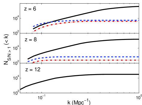
Figure 4.— Integrated number of Fourier pixels $N_{S/N>1}(k)$ with $k^{\prime}<k$ that have a ratio of the RMS signal to the RMS detector noise that is greater than unity for a $1000$ hr observation with $B=6~{}{\rm MHz}$. We use the specifications given in Table 1 and in §5 for MWA (dashed curve), LOFAR (dot-dashed curve), and SKA (solid curve). These curves do not include pixels with $k<2\pi/y$, since foregrounds will contaminate these pixels substantially. The 21 cm signal for this calculation is from a fully neutral medium in which $T_{s}\gg T_{\rm CMB}$. If the universe is partially ionized at $z=8$, the signal can be both larger and smaller than this (see Fig. 6). By a redshift of $12$, only SKA will have any high S/N pixels.

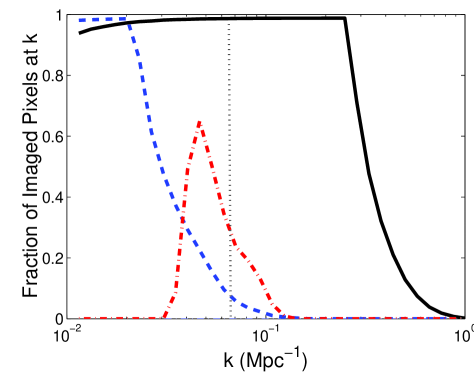
Figure 5.— Fraction of Fourier pixels for MWA (dashed curve), LOFAR (dot-dashed curve), and SKA (solid curve) that are “imaged”— that is, they have a ratio of RMS signal (assuming a neutral universe) to RMS detector noise that is greater than unity—after $1000$ hr of observation in a Fourier shell of radius $k$. The hatched vertical line marks the depth of this 6 MHz observation at $z=8$. Scales to the left of this should be wiped out by foregrounds. LOFAR can image a substantially higher fraction of pixels at the relevant $k$ than MWA, and SKA can image nearly all of its pixels up to $k=0.3\,{\rm Mpc}^{-1}$.

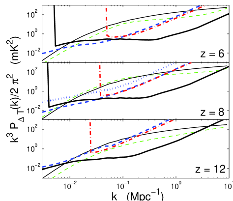
Figure 6.— Detector noise plus sample variance errors for a $1000$ hr observation on a single field in the sky, assuming perfect foreground removal, for MWA (thick dashed curve), LOFAR (thick dot-dashed curve), and SKA (thick solid curve), using the specifications given in Table 1 and in §5 and for bin sizes of $\Delta k=0.5\,k$. These errors are for the spherically averaged signal (see text for the discussion of this point). The hatched line in the middle panel represents MWA with a flat distribution of antennae rather than the fiducial $r^{-2}$ distribution. The detector noise dominates over sample variance for these sensitivity curves on almost all scales. The thin solid curve represents the spherically averaged signal for $\bar{x}_{i}\ll 1$ and $T_{s}\gg T_{\rm CMB}$. We use this curve to calculate the sample variance error. For comparison, the thin dashed curves show the signal from the FZH04 model when $\bar{x}_{i}$ is equal to $0.20$, $0.55$ and $0.75$ for $z=12,8$ and $6$, respectively.

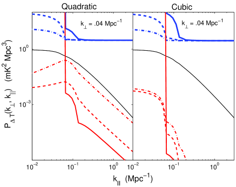
Figure 7.— Foreground removal for MWA for a $1000$ hr observation with $B=6~{}{\rm MHz}$. The thin solid curve shows $P_{\Delta T}({\boldsymbol{k}}_{\perp},k_{||})$ plotted as a function of $k_{||}$ for a neutral universe. The thick upper curves show the sensitivity to the signal $\delta P_{\Delta T}({\boldsymbol{k}}_{\perp},k_{||})$ if we remove the foregrounds using the method outlined in §4 in a band centered on the $6$ MHz cosmological signal processing window of $6,12,$ or $24~{}{\rm MHz}$ (solid, dashed or dot-dashed curves, respectively). Note that the sensitivity curves are above the curves for signal because this is the sensitivity to a single Fourier pixel ($N_{c}=1$). The lower curves show the function $Q_{{\boldsymbol{k}}_{\perp}}$, – the residual foreground level, – for each of the three processing window bandwidths (see §4). The foreground power in each panel is assumed to be a 1-$\sigma$ fluctuation of the model discussed in §4. The left panel shows a fit with a quadratic polynomial (${\rm n}=2$) and the right shows a fit with a cubic polynomial (${\rm n}=3$). While increasing ${\rm n}$ will always remove more of the foregrounds: it will also remove more of the cosmological signal as well. This can be seen in this plot by the reduced sensitivity to the signal at large scales. (In the absence of foregrounds and foreground cleaning, the sensitivity curves would be flat in this plot.)

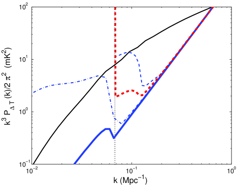
Figure 8.— Dimensionless 21 cm power spectrum for a neutral universe measured in a $6~{}{\rm MHz}$ band (thin solid curves) and the 1-$\sigma$ error for a $1000$ hr observation by MWA in the absence of foregrounds (thick solid curves), after foreground subtraction with a cubic polynomial at all $k_{\perp}$ in a $6~{}{\rm MHz}$ window (dashed curve) and in a $24~{}{\rm MHz}$ window (dot-dashed curve). The thick dashed curves is for a quadratic polynomial from a $6~{}{\rm MHz}$ band. The vertical hatched line denotes the scale of the $6~{}{\rm MHz}$ box. Foreground cleaning reduces the sensitivity at large scales. This plot illustrates that it makes a big difference how foregrounds are removed from the signal: experiments will want to remove the foregrounds over a fairly large bandwidth and with as low order a polynomial as possible.

6. Cosmology from the 21 cm Power Spectrum

Observations of high redshift 21 cm emission are capable of measuring $P_{\delta\delta}$ on smaller scales than current CMB experiments. Our calculations show that SKA can sensitively probe comoving megaparsec scales, which are also smaller than scales observed by galaxy surveys and comparable to scales probed with the Ly$\alpha$ forest. The sensitivity to smaller scales than the CMB may allow 21 cm observations to break degeneracies among cosmological parameters that are present in CMB constraints.

In this section, we utilize the sensitivity calculation described in §3 and §5 to estimate how well upcoming EOR interferometers can constrain cosmological parameters from $P_{\Delta T}$, and, in particular, whether these constraints will be competitive with CMB observations. We divide our discussion into three cases: (1) If density fluctuations dominate the signal (§6.1). This can happen if $\bar{x}_{i}\ll 1$ and $T_{\rm CMB}\ll T_{s}$ or if X-rays are responsible for the reionization of the Universe. (2) When the bubbles contaminate the $P_{\mu^{0}}$ and $P_{\mu^{2}}$ terms such that only $P_{\mu^{4}}$ and $P_{\mu^{6}}$, – which arises from the AP effect, – are pristine enough to measure cosmological parameters (§6.2). (3) On large scales at which neutral fraction fluctuations are important, but at which these fluctuations trace the density fluctuations (§6.3). Note that the analysis in this section does not assume any model for reionization.

It came to our attention that Bowman et al. (2005b) was performing a similar analysis for MWA and MWA5000. This paper, submitted concurrently with ours, pertains to when the signal is in the regime we discuss in §6.1. There are a few differences between our two approaches. In addition to cosmological parameters, Bowman et al. (2005b) fits to parameters for the foreground residuals as well as other observational parameters. Bowman et al. (2005b) also assumes a spherically symmetric $P_{\Delta T}$. Deviations from spherical symmetry enhance cosmological parameter constraints. Another important difference is that our analysis combines 21 cm observations with current and future CMB experiments. This can break parameter degeneracies present in these separate cosmological probes, and is important for assessing the true value of 21 cm observations for cosmology.

6.1. Density Fluctuations Dominate

We first concentrate on the signal in the case where the density fluctuations dominate over the spin temperature and neutral fraction fluctuations. This is the case in which 21 cm observations will be most sensitive to cosmological parameters. If reionization occurred at $z\approx 6.5$, as the Sloan quasars suggest (Becker et al., 2001; Fan et al., 2002), it is not altogether unlikely that upcoming interferometers will observe the signal in this regime. Models in which $\bar{x}_{i}=\zeta\,f_{\rm coll}$ have a significant period in which $\bar{x}_{i}\ll 1$. During this period, fluctuations in $x_{H}$ are unimportant. In addition, it is expected that at higher redshifts than those considered here, X-ray photons and shocks heat the gas in the IGM to well above the CMB temperature (Venkatesan et al., 2001; Chen & Miralda-Escudé, 2004). Ciardi & Madau (2003) argue that around $z=20$ the first stars will produce a large enough background in Ly$\alpha$ such that $T_{s}$ will be coupled to the kinetic temperature of the gas through the Wouthuysen-Field effect. If this is true, spin temperature fluctuations will be subdominant at the redshifts we consider.

Tables 2 and 3 quantify how the 21 cm signal can constrain some of the most interesting cosmological parameters: $\tau$, $\Omega_{w},w$, $\Omega_{m}\,h^{2}$, $\Omega_{b}\,h^{2}$, $n_{s}$, $\delta_{H}$, $\alpha_{s}$ and $\Omega_{\nu}$. The tilt $n_{s}$ we define to be the power law index of the primordial power spectrum at $k=0.05\,{\rm Mpc}^{-1}$ and $\alpha_{s}=dn_{s}(k)/d\log(k)$. The parameter $\delta_{H}$ is roughly the size of density fluctuations at the present day horizon scale (defined here such that the primordial power spectrum today $P(k)=2\pi^{2}\,\delta_{H}^{2}\,k^{n_{s}(k)}/[70\,{\rm km\,s^{-1}\,Mpc^{-1}}]^{3+n_{s}(k)}$). To construct the linear power spectrum used in this analysis, we employ the transfer function from the code CAMB. To get confidence intervals, we use the Fisher matrix formalism (Tegmark et al., 1997).

In the long term, MWA plans to increase the number of antenna panels from 500 to 5000. This array, MWA5000, will have a comparable collecting area to LOFAR and $10\%$ of the collecting area of SKA. To model MWA5000, we use an $r^{-2}$ distribution of antennae out to 1 km, similar to MWA, but with a larger flat core than MWA that extends out to $80\,{\rm m}$ rather than $20\,{\rm m}$. We also include MWA50K, which is another 10 times larger than MWA5000, but again built in the same mold as MWA. Correlating 50,000 antennae will be a significant computational challenge.

In Table 2, we calculate the 1-$\sigma$ errors on cosmological parameters for observations at $z=8$ in the case in which $\bar{x}_{i}\ll 1$ and $T_{s}\gg T_{\rm CMB}$, such that all the $\mu$ terms trace the density power spectrum. Unless otherwise noted, we perform the calculations in this section for an observation of $2000$ hr on two locations in the sky, or roughly $2$ productive years. Observations should generally be chosen to minimize the number of patches on the sky and maximize the duration for which each patch is observed because detector noise dominates the uncertainty at most scales. For the second generation of EOR interferometers, this is not necessarily the case, and sometimes parameter estimates are improved by choosing a different observing strategy.

Future observations have the potential to improve many of the current constraints on cosmological parameters. Two years of observation with MWA and LOFAR have trouble constraining a five parameter cosmology: $\Omega_{\Lambda}$, $\Omega_{m}\,h^{2}$, $\Omega_{b}\,h^{2}$, $n_{s}$, and the normalization parameter $\bar{x}_{H}\,\delta_{H}$ (see Table 2, note ‘b’). However, when combined with current CMB observations (WMAP, Boomerang, ACBAR [Arcminute Cosmology Bolometer Array Receiver], and CBI [Cosmic Background Imager]), both measurements by MWA and LOFAR are able to improve measurements of $\Omega_{\Lambda},\Omega_{m}\,h^{2},\Omega_{\nu},n_{s},$ and $\alpha_{s}$. MWA and LOFAR are not able to significantly improve the constraints from Planck. Unfortunately, $\bar{x}_{H}$ is not well constrained by measurements by MWA or by LOFAR when they are combined with current CMB observations. This is because the current uncertainty in cosmological parameters leads to substantial uncertainty in the amplitude of $P_{\delta_{L}\delta_{L}}$ at relevant scales. Planck will be able to refine the measurement of these parameters and the first generation of 21 cm experiments plus Planck will place tighter constraints on $\bar{x}_{H}$.

The second or third generation of 21 cm observations will be substantially more sensitive to the cosmology. By themselves, MWA5000, SKA and MWA50K can constrain a seven parameter cosmology that involves $\alpha_{s}$ and $\Omega_{\nu}$ in addition to the other five parameters we used for LOFAR and MWA (Table 2). Surprisingly, MWA5000 is comparably sensitive to SKA despite having $10$ times less collecting area. This is because SKA is not as centrally concentrated with only 20% of its antennae in the 1 km core while MWA5000 has 100%. Also, MWA5000 has a larger FOV than SKA, which results in smaller errors on large scales, scales at which these arrays are sample variance limited. Large scales probe the baryonic wiggles and therefore can provide substantial constraining power (Fig. 9). If we alter the observation for SKA to decrease the sample variance, – having it observe ten locations on the sky each for $400$ hr, – then SKA’s sensitivity is improved (see entries with asterisks in Table 2).

In combination with Planck, MWA5000 and SKA can improve constraints on $\Omega_{w}$, $\Omega_{m}\,h^{2}$, $n_{s},\alpha_{s}$ and $\Omega_{\nu}$, and MWA50K can do even better (Table 2). Because these observations probe smaller scales than the CMB, the parameters that affect the small scale behavior, namely $n_{s},\alpha_{s}$ and $\Omega_{\nu}$, show the most substantial improvement. In addition, as one changes the cosmological parameters in the conversion from ${\boldsymbol{u}}$ to ${\boldsymbol{k}}$, this distorts the measured power spectrum in k-space, providing an additional effect that can be used to constrain parameters. This is illustrated in Table 2: the constraints on SKA denoted with superscript ‘c’ are if we do not vary cosmological parameters in the conversion from ${\boldsymbol{u}}$ to ${\boldsymbol{k}}$. The uncertainty on $\Omega_{\Lambda}$, $\Omega_{m}\,h^{2}$, and $\Omega_{\nu}$ is substantially larger in this case.

Table 3 shows the sensitivity to cosmological parameters if the above scenario occurs at higher redshifts than $z=8$. MWA5000 is still sensitive to the signal at $z=10$, and its sensitivity falls off at $z=12$. Our design for SKA is unrealistically optimized for all considered redshifts. Because of this, SKA is more sensitive than MWA5000 at $z=12$, but it sensitivity is still falling due to the increasing sky temperature.

The uncertainty estimates in this section are for observations with $B=6~{}{\rm MHz}$. Experiments will be able to process a much larger bandwidth, and, if we are fortunate, nature could provide an even larger redshift slice in which density fluctuations dominate.

Figure 9.— Cosmic variance plus detector noise errors on the large scale modes of the spherically averaged power spectrum for SKA (thick error bars) and MWA5000 (thin error bars) after $1000$ hr of observation in a 6 MHz band. We accentuate the wiggles in $P_{\Delta T}(k)$ by subtracting a power spectrum that does not have baryonic wiggles $P^{\rm nw}_{\Delta T}(k)$. The vertical hatched line indicates the size of a 6 MHz box, approximately where we expect foregrounds to swamp the signal. The second generation of interferometers will be able to detect the wiggles at a few $\sigma$ significance level. MWA5000 is more sensitive than SKA to these features because of its larger FOV. The signal here is for $\bar{x}_{i}\ll 1$; the presence of HII bubbles may enhance these wiggles (§6.3).

Table 2Errors on cosmological parameter estimates when density fluctuations dominate the 21cm signal.

	$\tau$	$\Omega_{w}$	$w$	$\Omega_{m}\,h^{2}$	$\Omega_{b}\,h^{2}$	$n_{s}$	$\delta_{H}\times 10^{5}$	$\alpha_{s}$	$\Omega_{\nu}$	$\bar{x}_{H}$
	0.1	0.7	-1.0	0.14	0.022	1.0	3.91	0.0	0.0	1.0
LOFAR	-	0.07	-	0.11	0.03	0.11	5.0	-	-	-
MWA	-	0.06	-	0.09	0.02	0.09	4.2	-	-	-
MWA5000	-	0.005	-	0.008	0.002	0.03	0.37	0.010	0.007	-
SKA	-	0.005	-	0.009	0.002	0.06	0.51	0.016	0.015	-
SKA	-	0.11	-	0.042	0.003	0.07	2.0	0.017	0.08	-
SKA	-	0.004	-	0.007	0.002	0.03	0.32	0.010	0.008	-
MWA50K	-	0.002	-	0.004	0.001	0.01	0.17	0.004	0.002	-
CCMB	0.060	0.084	-	0.017	0.0014	0.072	0.29	0.039	0.12	-
CCMB+ LOFAR	0.057	0.050	-	0.010	0.0012	0.027	0.22	0.022	0.02	0.2
CCMB+ MWA	0.056	0.046	-	0.009	0.0011	0.021	0.22	0.022	0.02	0.2
CCMB+ MWA5000	0.048	0.005	-	0.003	0.0009	0.013	0.18	0.005	0.004	0.06
CCMB + SKA	0.048	0.005	-	0.003	0.0009	0.014	0.18	0.005	0.007	0.06
Planck	0.0050	0.029	0.09	0.0023	0.00018	0.0047	0.026	0.008	0.010	-
Planck +MWA5000	0.0046	0.017	0.06	0.0009	0.00012	0.0033	0.018	0.003	0.003	0.03
Planck + SKA	0.0046	0.021	0.08	0.0008	0.00012	0.0034	0.018	0.003	0.004	0.04
Planck + SKA	0.0046	0.017	0.07	0.0007	0.00012	0.0032	0.017	0.003	0.003	0.03
Planck + MWA50K	0.0045	0.007	0.03	0.0004	0.00010	0.0029	0.016	0.002	0.001	0.01

Table 3Same as Table 2, but for higher redshifts.

	$\tau$	$\Omega_{\Lambda}$	$\Omega_{m}\,h^{2}$	$\Omega_{b}\,h^{2}$	$n_{s}$	$\delta_{H}\times 10^{5}$	$\alpha_{s}$	$\Omega_{\nu}$	$\bar{x}_{H}$
	0.1	0.7	0.14	0.022	1.0	3.91	0.0	0.0	1.0
MWA5000 ($z=10$)	-	0.010	0.014	0.004	0.03	0.6	0.01	0.010	-
SKA ($z=10$)	-	0.007	0.010	0.003	0.03	0.4	0.01	0.009	-
MWA5000 ($z=12$)	-	0.019	0.030	0.008	0.07	1.4	0.03	0.016	-
SKA ($z=12$)	-	0.011	0.014	0.004	0.05	0.7	0.02	0.013	-
Planck	0.0049	0.011	0.0023	0.00017	0.0047	0.03	0.007	0.010	-
Planck + MWA5000 ($z=10$)	0.0047	0.007	0.0013	0.00013	0.0036	0.02	0.005	0.003	0.03
Planck + SKA ($z=10$)	0.0046	0.006	0.0011	0.00013	0.0035	0.02	0.004	0.003	0.03
Planck + MWA5000 ($z=12$)	0.0049	0.009	0.0017	0.00015	0.0040	0.02	0.007	0.004	0.04
Planck + SKA ($z=12$)	0.0047	0.007	0.0014	0.00014	0.0037	0.02	0.005	0.004	0.04

6.2. Neutral Fraction Fluctuations are Significant

In this section, we investigate whether it is possible to extract $P_{\mu^{4}}=\bar{x}_{H}^{2}\,P_{\delta_{L}\delta_{L}}$ from $P_{\Delta T}({\boldsymbol{k}})$ well enough to constrain cosmological parameters when ionized fraction fluctuations are important. Figure 10 shows the $z=8$ sensitivity curves for MWA and for SKA. The right panel is shown at the beginning of reionization ($\bar{x}_{i}=0.1$), when the density fluctuations are still the largest source of fluctuations. In this case, SKA will be sensitive to $P_{\mu^{4}}$ over 1-2 decades in $k$. Conversely, MWA is not sensitive to $P_{\mu^{4}}$. The left panel shows the opposite case, when the bubbles dominate ($\bar{x}_{i}=0.7$). In this case, MWA and SKA are both not sensitive to $P_{\mu^{4}}$. Both MWA and SKA can be sensitive to the $P_{\mu^{0}}$ over a range of scales. This analysis assumes that the fiducial cosmology is correct or else we could not measure $P_{\mu^{0}}$ and $P_{\mu^{4}}$, since we need to know the angular diameter distance and $H(z)$ to be able to convert ${\boldsymbol{u}}$ to ${\boldsymbol{k}}$.

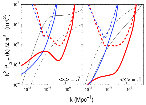
Figure 10.— Signal using the FZH04 model (thin curves) and detector noise plus cosmic variance errors (all other curves) at $z=8$ for a $2000$ hr observation combining two different fields of view, or roughly $2$ yr of observations, for the $P_{\mu^{0}}$ (solid curves) and $P_{\mu^{4}}$ (dashed curves) components of the signal. In the left panel $\bar{x}_{i}=0.7$, and in the right panel $\bar{x}_{i}=0.1$. We plot the sensitivity curves for MWA (medium-width curves) and for SKA (thick curves) with a binning width of $\Delta k=0.5\,k$. These curves assume that the angular diameter distance to $z$ and that the value of $H(z)$ are well constrained such that we can convert between ${\boldsymbol{u}}$ and ${\boldsymbol{k}}$. If this is not the case, there is also a $\mu^{6}$ term.

If the cosmology assumed in the conversion from ${\boldsymbol{u}}$ to ${\boldsymbol{k}}$ is incorrect, there will be an asymmetry in the measured depth versus measured angular size of an object (Alcock & Paczynski, 1979). As a result, features, such as the effective bubble size, will appear distorted in the 21 cm map [the AP effect]. Tests for this asymmetry can be used to put constraints on cosmological parameters. This effect is implicitly included in the analysis in §6.1 because we vary the cosmological parameters in the conversion from ${\boldsymbol{u}}$ to ${\boldsymbol{k}}$. To extract cosmology from $P_{\mu^{4}}$ alone, it is more subtle to include this effect.

The presence of this new angular dependence from the AP effect will contribute an additional term to the $\mu$ decomposition of $P_{\Delta T}$ (equation 6), which has a unique $\mu^{6}$ angular dependence with coefficient (Nusser, 2005; Barkana, 2005)

$$P_{\mu^{6}}({\boldsymbol{k}})=-\alpha\,\bar{x}_{H}^{2}\,(4\,P_{\delta_{L}\delta_{L}}-\frac{\partial P_{\delta_{L}\delta_{L}}}{\partial\log k}),$$ (43)

keeping terms to linear order in $\alpha$. Here $1+\alpha$ is the ratio of the true value of the Hubble constant times the angular diameter distance, $H(z)\,D_{A}(z)$, to the value assumed in the conversion from ${\boldsymbol{u}}$ to ${\boldsymbol{k}}$. This term arises from the coupling of the AP effect to $P_{\mu^{4}}$. If detected, the $\mu^{6}$ term would indicate a clear problem with the assumed cosmological model. The $P_{\mu^{0}}$, $P_{\mu^{2}}$ and $P_{\mu^{4}}$ terms are also affected by the AP effect. Since we currently cannot model $P_{\mu^{0}}$ and $P_{\mu^{2}}$ when the bubbles are important, the AP effect will not be detectable from these terms. However, we can model $P_{\mu^{4}}$ to zeroth order in $\alpha$. If the assumed cosmology is incorrect such that $\alpha\neq 0$, this term becomes (Barkana, 2005)

$$P_{\mu^{4}} = P^{\rm tr}_{\mu^{4}}+\alpha\,\left(5\,P^{\rm tr}_{\mu^{4}}-2\,P_{\mu^{2}}+\frac{\partial P_{\mu^{2}}}{\partial\log k}\right)$$ (44)

$$- \alpha_{\perp}\left(3\,P^{\rm tr}_{\mu^{4}}+\frac{\partial\,P^{\rm tr}_{\mu^{4}}}{\partial\log k}\right),$$

where $P^{\rm tr}_{\mu^{4}}$ is the true $\mu^{4}$ term (what we measure if $\alpha=0$) and $(1+\alpha_{\perp})$ is the ratio of the assumed angular diameter distance $D_{A}(z)$ to its true value. Since the $P_{\mu^{2}}$ is generally larger than $P^{\rm tr}_{\mu^{4}}$, the deviation from $P^{\rm tr}_{\mu^{4}}$ can be quite significant.

In Figure 11, we plot $P^{\rm tr}_{\mu^{4}}$ (solid curves), $P_{\mu^{6}}$ (dot-dashed curves), and $P_{\mu^{4}}-P^{\rm tr}_{\mu^{4}}$ (dashed curves) for $\bar{x}_{i}=0.2$ (thick curves) and $\bar{x}_{i}=0.55$ (thin curves) using the FZH04 analytic model at $z=8$. We take $\alpha=0.1$ and $\alpha_{\perp}=0.1$ to roughly match the current uncertainty in these parameters. The first generation of 21 cm arrays will not be sensitive to the AP effect or to $P_{\mu^{4}}$. The dashed and dot-dashed curves in Figure 11 that are labeled “Errors” represent the sensitivity curves for SKA to the $P_{\mu^{4}}$ and $P_{\mu^{6}}$ terms assuming $2$ yr of observation. SKA will not have the sensitivity to give a meaningful measurement of either $\alpha$ or $P_{\mu^{4}}$, but, after a sufficiently long integration, may be able to detect $P_{\mu^{6}}$. A similar conclusion holds for MWA5000.

Let us now make this analysis more quantitative. If we take the Fisher matrix $F_{ij}$ at a given $k$ for the parameters $P_{\mu^{0}},P_{\mu^{2}},P_{\mu^{4}},$ and $P_{\mu^{6}}$ (indexed 1 through 4), then marginalize the contaminated parameters $P_{\mu^{0}}$ and $P_{\mu^{2}}$, the Fisher matrix of just the parameters $P_{\mu^{4}}$ and $P_{\mu^{6}}$ is

$${\boldsymbol{F}}^{\prime}_{k}=\left(\begin{array}[]{cc}{{\boldsymbol{F}}^{-1}}_{33}&{{\boldsymbol{F}}^{-1}}_{34}\\ {{\boldsymbol{F}}^{-1}}_{43}&{{\boldsymbol{F}}^{-1}}_{44}\end{array}\right)_{k}^{-1}.$$ (45)

By the chain rule, it follows that the Fisher matrix for the cosmological parameters $\lambda_{1},...,\lambda_{n}$ obtained from just $P_{\mu^{4}}$ and $P_{\mu^{6}}$ (indexed by 1 and 2) is

$$F^{\prime\prime}_{ij}(k) = F^{\prime}_{11}\frac{\partial P_{\mu^{4}}}{\partial\lambda_{i}}\frac{\partial P_{\mu^{4}}}{\partial\lambda_{j}}+F^{\prime}_{12}\frac{\partial P_{\mu^{4}}}{\partial\lambda_{i}}\frac{\partial P_{\mu^{6}}}{\partial\lambda_{j}}$$ (46)

$$+ F^{\prime}_{21}\frac{\partial P_{\mu^{6}}}{\partial\lambda_{i}}\frac{\partial P_{\mu^{4}}}{\partial\lambda_{j}}+F^{\prime}_{22}\frac{\partial P_{\mu^{6}}}{\partial\lambda_{i}}\frac{\partial P_{\mu^{6}}}{\partial\lambda_{j}}.$$

In Table 4 we consider the scenario in which $\bar{x}_{H}=0.8$ and only $P_{\mu^{4}}$ and $P_{\mu^{6}}$ yield a pristine measure of the linear density power spectrum via equations (44) and (43). (While $P_{\mu^{4}}$ depends on $P_{\mu^{2}}$ to linear order in $\alpha$, since we can measure $P_{\mu^{2}}$, we can always use $P_{\mu^{4}}$ and $P_{\mu^{6}}$ to measure $P_{\delta\delta}$.) We assume that $\alpha$ and $\alpha_{\perp}$ are zero, but nonzero values do not change the results significantly. In this case, MWA5000 and SKA can improve constraints moderately on cosmological parameters obtained from current CMB data sets. However, they are unable to compete with Planck. The measurement of $P_{\mu^{4}}$ and $P_{\mu^{6}}$, when combined with Planck, will be most useful for measuring $\bar{x}_{H}$ rather than for constraining cosmological models. Two years of observation with SKA can constrain $\bar{x}_{H}$ to better than $10\%$. Even MWA50K is not able to sensitively constrain the signal on its own with this method.

SKA does fare better than MWA5000 for the analysis in this section, which was not the case in §6.1. This stems from MWA5000 being significantly more concentrated than SKA and therefore not as sensitive to small scale modes perpendicular to the LOS. These modes are important to be able to separate the different $\mu$ terms. Our design for MWA50K is very concentrated, like MWA5000, and so is also not optimal for measuring $P_{\mu^{4}}$ and $P_{\mu^{6}}$.

If one assumes some simple parameterization for $P_{xx}$ and $P_{x\,\delta}$ (or $P_{\mu^{0}}$ and $P_{\mu^{2}}$), rather than marginalizing over $P_{\mu^{0}}$ and $P_{\mu^{2}}$ for each $k$-bin as is done here, then perhaps one could measure $P_{\delta\delta}$ with more confidence.

Figure 11.— Plot of $k^{3}P(k)/2\pi^{2}$ for $P(k)$ equal to $P^{\rm tr}_{\mu^{4}}$ (solid curves), $P_{\mu^{6}}$ (dot-dashed curves) and $P_{\mu^{4}}-P^{\rm tr}_{\mu^{4}}$ (dashed curves) for $\bar{x}_{i}=0.2$ (thick curves) and $\bar{x}_{i}=0.55$ (thin curves) at $z=8$. Here we assume that $\alpha=0.1$ and $\alpha_{\perp}=0.1$. The dashed and dot-dashed curves, labeled “Errors,” are SKA’s errors for a $2$ yr observation on $P_{\mu^{4}}$ and $P_{\mu^{6}}$ when $\bar{x}_{i}=0.2$, computed with bins $\Delta k=0.5\,k$.

Table 4Errors on cosmological parameters estimates from 21 cm observations when only $P_{\mu^{4}}$ and $P_{\mu^{6}}$ are not contaminated by the bubbles.

	$\tau$	$\Omega_{\Lambda}$	$\Omega_{m}\,h^{2}$	$\Omega_{b}\,h^{2}$	$n_{s}$	$\delta_{H}\times 10^{5}$	$\alpha_{s}$	$\Omega_{\nu}$	$\bar{x}_{H}(z=8)$
	0.1	0.7	0.14	0.022	1.0	3.9	0.0	0.0	0.8
CCMB	0.060	0.084	0.017	0.0014	0.07	0.3	0.039	0.12	-
CCMB + MWA5000	0.058	0.066	0.011	0.0012	0.05	0.2	0.033	0.05	0.3
CCMB + SKA	0.057	0.062	0.011	0.0012	0.04	0.2	0.028	0.04	0.3
Planck	0.005	0.011	0.0023	0.00017	0.0047	0.03	0.007	0.010	-
Planck + MWA5000	0.005	0.011	0.0022	0.00017	0.0047	0.03	0.007	0.010	0.07
Planck + SKA	0.005	0.011	0.0022	0.00017	0.0047	0.03	0.007	0.010	0.07
Planck + MWA50K	0.005	0.010	0.0020	0.00017	0.0047	0.03	0.007	0.009	0.06

6.3. Large Scales

Up until now, we have ignored all components of the signal that are contaminated by the bubbles. On large scales, this may not be necessary. On scales much larger than the effective HII bubble size $R_{\rm eff}$, if the Poisson fluctuations owing to the bubbles are unimportant, the bubble fluctuations will trace the density fluctuations. Thus, when $k\ll R_{\rm eff}^{-1}$, we may have the relations

$$P_{xx}(k)\approx b_{1}^{2}\,P_{\delta\delta},~{}~{}~{}~{}~{}~{}P_{x\delta}(k)\approx b_{1}\,P_{\delta\delta}.$$ (47)

It is not necessarily the case with HII bubbles during reionization, as it is typically for galaxy surveys, that Poisson fluctuations are unimportant at large scales. If we include both the part of the signal that traces the $P_{\delta\delta}$ and the Poisson component, we can write the 21 cm power spectrum at large scales as

$$P_{\Delta T}({{\boldsymbol{k}}}) = \tilde{T}_{b}^{2}\,\{\left[\bar{x}_{H}^{2}+b_{1}^{2}-2\bar{x}_{H}\,b_{1}\right]+2\mu^{2}\,$$ (48)

$$\times\left[\bar{x}_{H}^{2}-\bar{x}_{H}\,b_{1}\right]+\mu^{4}\,\left[\bar{x}_{H}^{2}\right]\}P_{\delta\delta}+P_{\rm poi},$$

where $P_{\rm poi}$ is the Poisson contribution, which is constant in $k$. This type of decomposition may also hold when spin temperature fluctuations are important. On large scales we may again parameterize spin temperature fluctuations with the relation $\delta_{T_{s}}=b_{T_{s}}\,\delta$ for some constant $b_{T_{s}}$, and again the 21 cm power spectrum is proportional to $P_{\delta\delta}$. If we include the AP effect, terms enter with derivatives of $P_{\delta\delta}$.

Equation (48) is promising in that, when Poisson fluctuations are unimportant, there are effectively three unknowns ($b_{1},\bar{x}_{H}$ and $P_{\delta\delta}$) and three equations, since the $\mu^{0},\mu^{2}$ and $\mu^{4}$ components can, in principle, be measured. All three of the unknowns are very informative: $\bar{x}_{H}(z)$ tells us about the global reionization history, $b_{1}(z)$ indicates where the bubbles are located (i.e. overdense or average density regions), and of course $P_{\delta\delta}$ is quite interesting. In addition, $b_{1}$ can be much larger than unity, such that the signal is enhanced over that of a neutral medium.

There are several difficulties with extracting cosmology from these large scale modes. One difficulty is that modes larger than the width of the 21 cm survey will be contaminated by foregrounds. Another complication is that 21 cm interferometers will have progressively more trouble capturing terms of increasing order in $\mu$, which is necessary to separate the terms in equation (48). Despite these difficulties, it is probable that modes on scales near the baryonic wiggles ($k\sim 0.1~{}{\rm Mpc}^{-1}$) will be in this large scale regime. This is a region in k-space that contains much cosmological information and is also on scales where interferometers will be most sensitive to the $\mu$ decomposition of the signal (Fig. 10).

7. Discussion

In this paper, we have used the FZH04 analytical model of reionization to calculate the power spectrum of 21 cm brightness temperature fluctuations $P_{\Delta T}({\boldsymbol{k}})$, extending this calculation beyond calculations done in FZH04 by including redshift-space distortions. When $\bar{x}_{i}\lesssim 0.5$ or on smaller scales than the effective bubble size, these distortions are quite important and give the power spectrum a substantial anisotropy between modes parallel and perpendicular to the LOS. These distortions not only increase the signal, but may allow us to separate $P_{xx}$, $P_{x\delta}$ and $P_{\delta\delta}$, facilitating the measurement of the size and bias of the HII bubbles and perhaps the spectrum of density fluctuations in the Universe. We show that higher order terms may complicate the separation of $P_{\Delta T}$ when the ionized fraction is significant.

To quantify the detectability of $P_{\Delta T}({\boldsymbol{k}})$, and in particular $P_{\delta\delta}$, we make realistic sensitivity estimates for LOFAR, MWA and SKA. The most important parameter for these interferometers is the collecting area. But, this is not to say that the other factors that go into the design are unimportant. We agree with the conclusion of Bowman et al. (2005a) that, everything else being equal, arrays with denser cores will be more sensitive to $P_{\Delta T}({\boldsymbol{k}})$. This is because modes along the LOS can be detected by even the shortest baselines, and arrays with cores have more of these shorter baselines. The antenna size can also have a similar effect: arrays that have large antennae cannot pack them as closely together as arrays with small antennae. As a result, they will not sample the shorter baselines as well. Smaller antennae also provide a larger FOV, which will aid statistical detections of the signal. Because the current design for LOFAR does not include the shorter baselines that the design for MWA has and because the design for LOFAR results in a much smaller FOV, we find that, despite differences in collecting area, LOFAR and MWA will be comparably sensitive to $P_{\Delta T}({\boldsymbol{k}})$ at most redshifts. This is not to say that this will be the case when these instruments are actually deployed. Since none of the discussed 21 cm arrays have begun construction, their designs can still be optimized.

Even with an optimally constructed radio interferometer, the removal of foregrounds that are $10^{4}$ times larger than the 21 cm fluctuations will be a serious challenge. In this paper, we find that foregrounds will contaminate the signal on scales greater than the depth of the slice used to construct the 21 cm power spectrum. At most scales smaller than this, we are optimistic that foregrounds can be cleaned below the signal. On such scales, we show that fitting a quadratic or cubic polynomial to the observed visibilities in the frequency direction has little difficulty cleaning a realistic model for foregrounds. It does not appear to be the case, as was claimed by Oh & Mack (2003) and Gnedin & Shaver (2004), that foregrounds will contaminate all angular modes beyond repair.

Applying our calculation for the detector noise and foreground power spectrum, we find that MWA and LOFAR will not be sensitive to the $P_{\mu^{4}}$ component of $P_{\Delta T}({\boldsymbol{k}})$. This component is particularly interesting because it traces the linear-theory density power spectrum. However, these interferometers will be sensitive to $P_{\mu^{0}}$, which probably will tell us more about the astrophysics of reionization than about cosmology, except perhaps for very small ionization fractions. MWA5000 and SKA will be moderately sensitive to $P_{\mu^{4}}$ and $P_{\mu^{6}}$, but not sensitive enough to provide competitive constraints on cosmological parameters. We find that only if there exists a time when density fluctuations dominate $P_{\Delta T}$, will upcoming probes of 21 cm emission be able to place competitive constraints on cosmological parameters. In addition, planned 21 cm interferometers will not be very sensitive to the signal for $z\gtrsim 12$. The is primarily because detector noise fluctuations are proportional to $T_{\rm sky}(z)$, which scales as $(1+z)^{2.6}$.

If there is a period where density fluctuations dominate $P_{\Delta T}$, a $2$ yr observation with MWA5000 plus Planck can give the constraints $\delta\Omega_{w}=0.0017$ (a $1.7$ times smaller uncertainty than from Planck alone), $\delta w=0.06$ ($1.5$ times), $\delta\Omega_{m}h^{2}=0.0009$ ($2.5$ times), $\delta\Omega_{b}h^{2}=0.00012$ ($1.5$ times), $\delta n_{s}=0.0033$ ($1.4$ times), $\delta\alpha_{s}=0.003$ ($2.7$ times), $\delta\Omega_{\nu}=0.003$ ($3$ times) and $\delta x_{H}=0.03$. SKA plus Planck yield similar constraints and MWA50K can do even better. However, if $\tau=0.17$, as suggested by WMAP, and reionization began at $z\approx 20$, observations of the signal at scales much larger than the effective bubble size may be the most promising direct method to probe cosmology (§6.3).

Observations must overcome many additional challenges beyond those that have been discussed in this paper. Issues that we have not addressed include contamination by radio recombination lines, terrestrial radio interference, the residuals left from wave front corrections for a turbulent atmosphere, and the enormous data analysis pipeline needed to analyze potentially larger data sets than those from current experiments. The 21 cm signal will also be affected by gravitational lensing by intervening material (Zahn & Zaldarriaga, 2005; Mandel & Zaldarriaga, 2005). If taken into account, this effect can further improve cosmological parameter estimates (Zahn & Zaldarriaga, 2005).

Cosmic variance sets a limit on how well we can constrain cosmological models with the CMB. Because 21 cm emission can be observed as a function of redshift, this signal allows us to measure many more independent modes than is possible with the CMB. We have seen that cosmological parameters are extractable from 21 cm emission. In an ideal case in which reionization begins at relatively low redshifts, upcoming interferometers may be able to compete with future CMB experiments such as Planck. If reionization begins at higher redshifts or if the spin temperature fluctuations are important, a more sensitive interferometer will be required than those that are currently planned to be able to compete with CMB parameter constraints. Regardless of how reionization actually proceeded, high-redshift 21 cm emission has the potential to become a valuable probe of cosmology.

We thank Judd Bowman, Bryan Gaensler, Adam Lidz and Miguel Morales for useful discussions. This work was supported in part by NSF grants ACI 96-19019, AST 00-71019, AST 02-06299, and AST 03-07690, and NASA ATP grants NAG5-12140, NAG5-13292, and NAG5-13381.

Appendix A The Effect of Evolution

Observations must have a large enough bandwidth to provide adequate signal-to-noise, but the larger the bandwidth, the more the signal will evolve along the LOS direction of the 21 cm map. During reionization this evolution includes (1) density inhomogeneities growing with time and (2) the average 21 cm brightness temperature declining as the Universe expands and the bubbles grow and occupy progressively more space. The latter should dominate over the former owing to the relatively short timescales during which the ionization fraction changes by order unity. Since the Universe is evolving across modes along the LOS and is not evolving for those transverse to the LOS, this evolution will break the spherical symmetry of the signal and potentially make it more difficult to observe $P_{\mu^{0}}$, $P_{\mu^{2}}$, $P_{\mu^{4}}$ and $P_{\mu^{6}}$. In this section, we attempt to quantify the potential size of this effect for an idealized case.

Very simple models for reionization set $P_{\Delta T}=b^{2}\,P_{\delta\delta}$ where $b$ is the effective bias. This parameterization is certainly not correct, and the bias will have a scale dependence for scales around the size of the bubbles. This model for the power spectrum is reasonable at the beginning of reionization, when density fluctuations dominate, and on much larger scales than the bubbles . Fortunately, these are the regimes in which the cosmological information is most readily extractable from the signal (see §6.1 and §6.3).

With the assumption that $P_{\Delta T}=b^{2}\,P_{\delta\delta}$, we can write an expression for the power spectrum in a region of width $2\,\Delta r$

$$P_{\Delta T}({{\boldsymbol{k}}})=\langle\frac{1}{\Delta V}\,\mathop{\int_{\Delta V}}d^{3}{\boldsymbol{r}}d^{3}\boldsymbol{\epsilon}\,F(r_{||})\,\delta_{0}({{\boldsymbol{r}}})\,F(r_{||}+\epsilon_{||})\,\delta_{0}({{\boldsymbol{r}}}+{\bf\epsilon})\exp(-{\it i}{{\boldsymbol{k}}}\cdot{\bf\epsilon}){\rangle},$$ (A1)

where $\Delta V$ is specified in the LOS direction by the conditions ${|r_{||}-\bar{r}_{||}|<\Delta r}$ and ${|r_{||}+\epsilon_{{||}}-\bar{r}_{||}|<\Delta r}$ and $r_{||}$ is the projection of $r$ along the LOS and is assumed to be much larger than $\Delta r$ in the angular directions.. To constants of order unity, $F=b(z)\,(1+z)^{-1/2}$ [the factor of $(1+z)^{-1/2}$ owes to the evolution of $\bar{T}_{b}$ as well as the growth factor], and $\delta_{0}$ are the linear density fluctuations at $z=0$ [$\delta_{L}(z)=G(z)\,\delta_{0}$, where $G$ is the growth factor]. Here the subscript ${||}$ indicates the LOS direction. The $\langle\rangle$ indicates an ensemble average of maps, and $\langle\delta_{0}({\boldsymbol{r}})\delta_{0}({\boldsymbol{r}}+{\bf\epsilon})\rangle=\zeta_{\delta_{0}\delta_{0}}({\bf\epsilon})$ in which $\xi_{\delta_{0}\delta_{0}}$ is the linear density field correlation function. The Fourier transform of $\xi_{\delta_{0}\delta_{0}}$ is $P_{\delta_{0}\delta_{0}}$. By the Fourier transform convolution identity, equation (A1) is equivalent to

$$P_{\Delta T}({{\boldsymbol{k}}})=\int dk_{||}^{\prime}\,\tilde{W}(k_{||}^{\prime})\,P_{\delta_{0}\delta_{0}}({{\boldsymbol{k}}}-{{\boldsymbol{k}}}^{\prime}),$$ (A2)

where

$$\tilde{W}(k_{||})=\frac{1}{2\,\Delta r}\int_{\Delta V_{||}}dr_{||}\,d\epsilon_{{||}}\,F(r_{||})\,F(r_{||}+\epsilon_{{||}})\,\exp(-{\it i}k_{||}\,\epsilon_{{||}}).$$ (A3)

Prior to reionization, $b=1$ and $\tilde{W}(k)$ is almost identical to the window function for a top-hat in real space. Since this window function peaks when its argument is near zero, for large ${\boldsymbol{k}}$, then $P_{\Delta T}({{\boldsymbol{k}}})\approx P_{\delta_{0}\delta_{0}}({\boldsymbol{k}})\,\int dk^{\prime}\,\tilde{W}(k^{\prime})$. This is exactly what we should expect; in this limit, we are effectively averaging over modes located at different redshifts, such that only the amplitude of the observed power spectrum is affected by evolution. The difference between this window function for a universe in which the ionized fraction is and is not changing will indicate the degree to which the spherical symmetry is affected by the evolving ionized fraction. For example, if the window function becomes less peaked, then the spherical symmetry of more modes is affected by the evolving ionized fraction. In cases in which the window function is unaffected, this means that evolution only affects the normalization of the power spectrum through a factor of $\int dk^{\prime}\,\tilde{W}(k^{\prime})$. While the normalization is also interesting, it is degenerate with the parameters $\bar{x}_{H}$, $b_{1}$ (the linear bias of the bubbles) and $\sigma_{8}$ and therefore is less important.

Figure 12 plots the window function at $z=10$ for maps with comoving depth $110$ and $230~{}{\rm Mpc}$ ($\Delta z=0.5$ and 1) for a neutral universe (solid curve) and two cases in which $b(z)\propto[m(z-10)+1]$ for $m=0.5$ and $1$. This is a conservative choice; such a quick change of $b$ is much larger than models predict at the beginning of reionization. Figure 12 demonstrates that the window function is virtually unaltered for three of the four cases. Only in the most extreme case, where $m(z-10)+1$ varies from 0 to 1 within the map, is the window function significantly altered. Therefore, the evolution of the signal for this simple model weakly breaks the spherical symmetry of the signal.

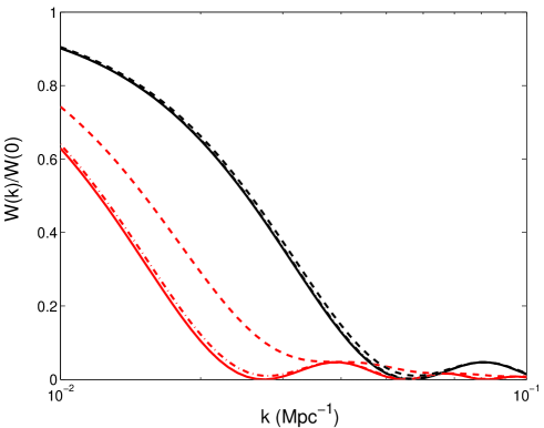
Figure 12.— Window function $\tilde{W}(k)$, defined in equation (A3), for maps of comoving depths $110~{}{\rm Mpc}$ (outer curves) and $230$ Mpc (inner curves) at $z=10$ . We plot the window function for a universe prior to reionization $b(z)={\rm constant}$ (solid curves) and for when the universe is starting to be ionized (quickly) with $b(z)\propto[m(z-10)+1]$ for $m=0.5\,{\rm~{}and~{}}\,1$ (dot-dashed and dashed curves, respectively).

Appendix B Angular Averaged Sensitivity

The spherically averaged signal is obtained by summing up all pixels in a shell with the same $|{\boldsymbol{k}}|$. If $\Delta k=\epsilon k$, it follows from equation (24) that the error on $P_{\Delta T}(k)$ from a measurement of all pixels in a shell with constant $k$ is given by

$$\delta P_{\Delta T}(k) = \left[\sum_{\theta}~{}\left(\frac{1}{\delta P_{\Delta T}(k,\theta)}\right)^{2}\right]^{-1/2}$$ (B2)

$$\approx \left[k^{3}\,\int_{\arccos[\min(\frac{yk}{2\pi},1)]}^{\arcsin[\min(\frac{k_{*}}{k},1)]}~{}d\theta\,\sin(\theta)\,\frac{1}{\left(D\,P_{\rm 21cm}(k)+\frac{E}{n(k\sin(\theta))}\right)^{2}}\right]^{-1/2},$$

$$D=\sqrt{\frac{(2\pi)^{2}\,A_{e}}{\lambda^{2}\,x^{2}\,y\,\epsilon}}~{}~{}~{}~{}E=\frac{2\pi\,\sqrt{x^{2}y}\,\lambda^{3}\,T_{\rm sys}^{2}}{\sqrt{\,\epsilon}\,A_{e}^{3/2}\,(B\,t_{0})},$$

where $k_{*}$ corresponds to the longest wavevector perpendicular to the LOS probed by the array. In equation (B2), the lower bound of the integrand reflects the sharp cutoff in the number of pixels imposed for wavelengths that do not fit in the width of the box, $y$. Some interferometers, such as LOFAR, will be able to observe $N_{\rm point}$ separate fields of view simultaneously. To include this effect, one can simply divide equation (B2) by $\sqrt{N_{\rm point}}$.

To gain intuition into the scalings of equation (B2), let us take a top-hat distribution of baselines with density $\rho(\lambda)$ in the limit in which the detector noise dominates such that we can set $P_{\rm 21cm}=0$ in equation (B2). In this case, we can evaluate the integral in equation (B2), which yields

$$\delta P_{\Delta T}(k) = E\,\left(\min[\frac{yk}{2\pi},1]\right)^{-1/2}\,\rho^{-1}\,k^{-3/2}~{}~{}~{}~{}k<k_{*}$$ (B3)

$$= E\,\rho^{-1}\,k^{-3/2}\,(1-\frac{\sqrt{k^{2}-k_{*}^{2}}}{k})^{-1/2}~{}~{}~{}~{}k>k_{*}.$$ (B4)

When $k\gg k_{*}$, $\delta P_{\Delta T}(k)\propto k^{-0.5}$.

References

- Alcock & Paczynski (1979) Alcock, C. & Paczynski, B. 1979, Nature, 281, 358
- Barkana (2005) Barkana, R. 2006, MNRAS, 372, 259
- Barkana & Loeb (2005a) Barkana, R. & Loeb, A. 2005a, ApJ, 624, L65
- Barkana & Loeb (2005b) —. 2005b, ApJ, 626, 1
- Becker et al. (2001) Becker, R. H. et al. 2001, AJ, 122, 2850
- Bharadwaj & Ali (2004) Bharadwaj, S. & Ali, S. S. 2004, MNRAS, 352, 142
- Bond et al. (1991) Bond, J. R., Cole, S., Efstathiou, G., & Kaiser, N. 1991, ApJ, 379, 440
- Bowman et al. (2005a) Bowman, J. D., Morales, M. F., & Hewitt, N. J. 2005a, Submitted to ApJ (astro-ph/0507357)
- Bowman et al. (2005b) —. 2005b, Submitted to ApJ
- Bromm et al. (2001) Bromm, V., Kudritzki, R. P., & Loeb, A. 2001, ApJ, 552, 464
- Carilli & Rawlings (2004) Carilli, C. L. & Rawlings, S. 2004, astro-ph/0409274
- Chen & Miralda-Escudé (2004) Chen, X. & Miralda-Escudé, J. 2004, ApJ, 602, 1
- Ciardi & Madau (2003) Ciardi, B. & Madau, P. 2003, ApJ, 596, 1
- Ciardi et al. (2003) Ciardi, B., Stoehr, F., & White, S. D. M. 2003, MNRAS, 343, 1101
- Ciardi et al. (2005) Ciardi, B., Scannapieco, E., Stoehr, F., Ferrara, A., Iliev, I. T., Shapiro, P. R. Submitted to MNRAS (astro-ph/0511623)
- de Vos (2004) de Vos, M. 2004, http://www.lofar.org/PDF/LOFAR-P1-Baseline2.0.pdf
- Di Matteo et al. (2002) Di Matteo, T., Perna, R., Abel, T., & Rees, M. J. 2002, ApJ, 564, 576
- Fan et al. (2002) Fan, X., Narayanan, V. K., Strauss, M. A., White, R. L., Becker, R. H., Pentericci, L., & Rix, H.-W. 2002, AJ, 123, 1247
- Field (1958) Field, G. B. 1958, Proc. IRE, 46, 240
- Field (1959) —. 1959, ApJ, 129, 525
- Furlanetto et al. (2005) Furlanetto, S. R., McQuinn, M., & Hernquist, L. 2005, MNRAS, 1043
- Furlanetto & Oh (2005) Furlanetto, S. R. & Oh, S. P. 2005, MNRAS, 363, 1031
- Furlanetto et al. (2004) Furlanetto, S. R., Zaldarriaga, M., & Hernquist, L. 2004, ApJ, 613, 1 [FZH04]
- Furlanetto et al. (2004b) Furlanetto, S. R., Zaldarriaga, M., & Hernquist, L. 2004b, ApJ, 613, 16
- Gnedin & Shaver (2004) Gnedin, N. Y. & Shaver, P. A. 2004, ApJ, 608, 611
- Hobson et al. (1995) Hobson, M. P., Lasenby, A. N., & Jones, M. 1995, MNRAS, 275, 863
- Iliev et al. (2002) Iliev, I. T., et al 2002, ApJ, 572, 123L
- Iliev et al. (2005) Iliev, I. T., Mellema, G., Pen, U. L., Merz, H., Shaprio, P., & Alvarez, M. A. 2005, Submitted to MNRAS (astro-ph/0512187)
- Kohler et al. (2005) Kohler, K. & Gnedin, N. Y. 2005, BAAS, 37, 1417
- Lacey & Cole (1993) Lacey, C. & Cole, S. 1993, MNRAS, 262, 627
- Mandel & Zaldarriaga (2005) Mandel, K. & Zaldarriaga, M. 2005, Submitted to ApJ (astro-ph/0512218)
- McQuinn et al. (2005) McQuinn, M., Furlanetto, S. R., Hernquist, L., Zahn, O., & Zaldarriaga, M. 2005, ApJ, 630, 643
- Morales (2005) Morales, M. F. 2005, ApJ, 619, 678
- Nusser (2005) Nusser, A. 2005, MNRAS, 364, 743
- Oh (2001) Oh, S. P. 2001, ApJ, 553, 499
- Oh & Mack (2003) Oh, S. P. & Mack, K. J. 2003, MNRAS, 346, 871
- Pen et al. (2005) Pen, U. L., Wu, X. P., & Peterson, J. 2005, Submitted to CJAA (astro-ph/0404083)
- Press & Schechter (1974) Press, W. H. & Schechter, P. 1974, ApJ, 187, 425
- Rohlfs & Wilson (2004) Rohlfs, K. & Wilson, T. L. 2004, Tools of Radio Astronomy (Berlin: Springer)
- Santos et al. (2005) Santos, M. G., Cooray, A., & Knox, L. 2005, ApJ, 625, 575
- Scott & Rees (1990) Scott, D. & Rees, M. J. 1990, MNRAS, 247, 510
- Shapiro et al. (2003) Shapiro, P., Ilian, I. T., Raga, A. C. 2004, MNRAS, 348, 753
- Shapiro et al. (2005) Shapiro, P., Ahn, K., Alvarez, M. A., Iliev, I. T., Martel, H., & Ryu, D. 2005, submitted to ApJ(astro-ph/0512516)
- Shaver et al. (1999) Shaver, P. A., Windhorst, R. A., Madau, P., & de Bruyn, A. G. 1999, A&A, 345, 380
- Sheth (1998) Sheth, R. K. 1998, MNRAS, 300, 1057
- Sokasian et al. (2003) Sokasian, A., Abel, T., Hernquist, L., & Springel, V. 2003, MNRAS, 344, 607
- Sokasian et al. (2004) Sokasian, A., Yoshida, N., Abel, T., Hernquist, L., & Springel, V. 2004, MNRAS, 350, 47
- Spergel et al. (2003) Spergel, D. N. et al. 2003, ApJS, 148, 175
- Tegmark (1997) Tegmark, M. 1997, Phys. Rev. D, 55, 5895
- Tegmark et al. (2000) Tegmark, M., Eisenstein, D. J., Hu, W., & de Oliveira-Costa, A. 2000, ApJ, 530, 133
- Tegmark et al. (1997) Tegmark, M., Taylor, N. A., & Heavens, A. F. 1997, ApJ, 455, 1
- Tozzi et al. (2000) Tozzi, P., Madau, P., Meiksin, A., & Rees, M. J. 2000, ApJ, 528, 597
- Venkatesan et al. (2001) Venkatesan, A., Giroux, M. L., & Shull, J. M. 2001, ApJ, 563, 1
- Wang & Hu (2005) Wang, X. & Hu, W. 2005, Submitted to ApJ (astro-ph/0511141)
- Wang et al. (2005) Wang, X., Tegmark, M., & Santos, M. 2006, ApJ, 650, 529
- White et al. (1999) White, M. et al. 1999, ApJ, 514, 12
- Wouthuysen (1952) Wouthuysen, S. A. 1952, AJ, 57, 31
- Zahn & Zaldarriaga (2005) Zahn, O. & Zaldarriaga, M. 2005, ApJ in press (astro-ph/0511547)
- Zaldarriaga et al. (2004) Zaldarriaga, M., Furlanetto, S. R., & Hernquist, L. 2004, ApJ, 608, 622