Simple, Accurate, Approximate Orbits in the Logarithmic and
a Range of Power-Law Galactic Potentials

Abstract

Curves in a family derived from powers of the polar coordinate formula for ellipses are found to provide good fits to bound orbits in a range of power-law potentials. This range includes the well-known $1/r$ (Keplerian) and logarithmic potentials. These approximate orbits, called p-ellipses, retain some of the basic geometric properties of ellipses. They satisfy and generalize Newton’s apsidal precession formula, which is one of the reasons for their surprising accuracy. Because of their simplicity the p-ellipses make very useful tools for studying trends among power-law potentials, and especially the occurence of closed orbits. The occurence of closed or nearly closed orbits in different potentials highlights the possibility of period resonances between precessing, eccentric orbits and circular orbits, or between the precession period of multi-lobed closed orbits and satellite periods. These orbits and their resonances promise to help illuminate a number of problems in galaxy and accretion disk dynamics.

1 Introduction

In recent decades, the recognition that galaxies are surrounded by extended halos of dark matter has spurred a greatly increased interest in the structure of orbits in gravitational potentials that are shallower than the Keplerian $1/r$ potential (e.g., Binney & Tremaine 1987, Bertin 2000). Similarly, the mass distribution in galactic bulges and elliptical galaxies is also extended, and the potential shallower than the Keplerian one. The logarithmic potential, $\Phi\propto\ln(r)$, is among the simplest and most studied examples of such a shallow potential, and will be used as a primary example in this work. The celestial mechanics of such potentials is not nearly as well developed as the centuries old literature of the classical Kepler-Newton potential, but there has been much recent progress (see Boccaletti & Pucacco 1996 and Contopoulos 2002).

The orbits in most physically relevant potentials can be numerically integrated very quickly and accurately, except near singularities and resonances. Direct numerical integration has provided much information about orbit families in both general symmetric, and non-axisymmetric potentials relevant to barred galaxies (including non-axisymmetric logarithmic potentials, see e.g., Miralda-Escude & Schwarzschild 1989).

There has also been much progress in the areas of analytic approximation and global properties of orbits in non-Keplerian potentials, and power-law potentials in particular. Concerning global properties, Stoica & Font (2003) have studied the topology of energy surfaces of the logarithmic potential and derived a complete qualitative description of orbits in the axisymmetric case. They also proved that orbits are centrophobic for the non-axisymmetric case as well. Valluri et al. (2005) have presented extensions of Newton’s apsidal precession theorem (Newton, 1687) for power-law potentials, and in the process found no evidence for cases of zero precession at high eccentricities. The work below provides further support for that conjecture.

With regard to analytic approximation, we note first of all that classical epicyclic approximations are the most well developed (e.g., see Binney & Tremaine 1987, Dehnen 1999, and Contopoulos 2002). Beyond this, Contopoulos & Scimenis (1990) have used the multiple Fourier series method of Prendergast (1982) to find orbit families and to derive accurate orbit approximations for the symmetric and non-axisymmetric logarithmic potentials. Adams & Block (2005) have examined spirograph or epicycloid orbit approximations and found that they accurately fit a wide range of orbits in the Hernquist and other halo potentials (with only two “spirograph” circles). The spirograph or epicycloid approximation is formally distinct from the epicyclic approximation, though similar in that they both can be extended to arbitrary accuracy.

More recently, Touma & Tremaine (1997) developed a relatively simple symplectic mapping for non-axisymmetric potentials that captures the behavior of orbits in these potentials. The map is based on the approximation that orbital evolution is driven by two processes: apsidal precession in the axisymmetric part of the potential, and torques by the non-axisymmetric potential, concentrated at apoapse. Because this symplectic map is based on apsidal precession, the Valluri et al. paper and the results below on precession complement it.

With this recent work the knowledge base on orbits in galaxy potentials (and similarly shallow potentials in galaxy groups and clusters) has become quite extensive. However, the basis of much of classical celestial mechanics (and many specific approximation schemes) is the simplicity of Kepler’s elliptical orbit solution. The conceptual and analytical foundation of galactic dynamics and other fields that use power-law potentials is inevitably weaker without such simple orbital solutions. Unfortunately, mechanics textbooks teach us that analytic orbital solutions only exist in a few special cases among the power-law forces (Goldstein 1980, Danby 1988). The simple epicyclic approximation provides a versatile computational tool, but with limitations as a conceptual tool if multiple or large epicycles are needed for accurate calculations (e.g., Contopoulos 2002, section 3.1). The references above show that other accurate approximations have been developed, but they are complex.

The purpose of this paper is to present a family analytic orbit approximations for the logarithmic and other spherically symmetric, or axisymmetric potentials. These orbit functions are simply powers of precessing ellipses, and so, very simple indeed. Nonetheless, for small-to-moderate eccentricities, they are also surprisingly accurate. For the logarithmic potential, the approximate orbits librate around accurate numerical solutions, but do not diverge from them over time. Equally surprising, these approximate solutions extend continuously across all members of a family of potentials that range from the Keplerian potential to potentials with slightly rising rotation curves. Although they do not provide complete analytic solutions, their simplicity and accuracy allow them to fill a large part of the role of simple analytic solutions in providing a readily understandable conceptual picture of the nature of orbits in these potentials and the relations between them.

2 Equations for Core Plus Power-Law Halo Potentials

2.1 Potentials

In this section I present the basic equations and dimensionless parameters that will be used in the following sections. All of the potentials used in this work give accelerations described by the equation,

$$g(r)=\frac{-GM_{*}r}{(\epsilon^{2}+r^{2})^{n}},$$

$$\mbox{with}\ M(r)=\frac{r^{3}}{(\epsilon^{2}+r^{2})^{n}}M_{*},$$ (1)

$$\mbox{so}\ M_{*}=2^{n}M(\epsilon)\epsilon^{2n-3},$$

where $\epsilon$ is a core scale length and $M_{*}$ is the constant scale mass of the potential. The last equation relates the scale mass to the mass contained within the scale length. The acceleration of equation (1) has many useful limiting forms. First of all, when $r\gg\epsilon$, the acceleration increases linearly with radius, as does the circular orbit velocity. Thus, we have a solid-body rotation at small radii. In the special case of $n=3/2$ we have the well-known Plummer model. The potential corresponding to this acceleration is also related to those studied in general scattering theory (see e.g., Newton 1966).

Secondly, when $r\gg\epsilon$, we have the power-law limit, $g\propto 1/r^{n-1}$. It is convenient to define $n=1+\delta$, so that the exponent of $r$ is $\delta$ in this limit. Three interesting special cases are: 1. $n=0$, $\delta=-1$, circular velocity $v_{cir}\propto r$, 2. $n=1$, $\delta=0$, circular velocity $v_{cir}=$ constant, and 3. $n=3/2$, $\delta=1/2$, circular velocity $v_{cir}\propto r^{-1/2}$. Clearly, these cases correspond to linearly rising, flat and Keplerian rotation curves, respectively.

The potential and density equations corresponding to the acceleration of equation (1) are given by,

$$\Phi(r)=\frac{-GM_{*}}{2\delta\left(\epsilon^{2}+r^{2}\right)^{\delta}},$$

$$\rho=\frac{3M_{*}}{4\pi}\ \left[\frac{\epsilon^{2}+\left(\frac{1-2\delta}{3}\right)r^{2}}{\left(\epsilon^{2}+r^{2}\right)^{2+\delta}}\right].$$ (2)

The latter equation shows that density is approximately constant within the core. This equation yields negative densities when $\delta>1/2$, and $r^{2}>(3/(2\delta-1))\epsilon^{2}$, i.e., at large radii in potentials where the outer falloff is more rapid than the Keplerian one. Such potentials are not very relevant to galaxy dynamics. However, some examples of them are used below, so it is worth noting that the density is positive out to quite large radii for potentials where $\delta$ is only slightly larger than $1/2$.

Currently, both observations (e.g., Díaz et al. 2005) and numerical structure formation models support the idea that halo profiles are universal. Among the most popular forms are the Navarro, Frenk, & White (1997, henceforth NFW) and Hernquist (1990) profiles. The density functions of both these profiles have a charateristic scale length, but they are also singular at the center, so their scale length does not correspond to a core size as in equation (2). Power-law potentials that are singular at the center will also be considered below. However, there is evidence that the core density profiles of some galaxies are flat rather than singular (e.g., Donato, Gentile, & Salucci 2004 and references therein). Henriksen (2005) has recently argued that the NFW state is a partially relaxed state, that in isolation ultimately relaxes to a core profile with solid body rotation. (For other recent views on the origin of halo profiles see the recent works of An & Evans 2005, Dehnen & McLaughlin 2005, and Lu et al. 2005.)

At large radii the NFW and Hernquist density profiles fall off as $1/r^{3}$. This is also true of the profile of equation (2) when $\delta=1/2$. I would emphasize, however, that the goal of this work is not to study how well a certain class of orbital approximations applies to specific halo potentials, Rather it is to describe how this family of approximations works in a range of simple schematic potentials, such as those of equation (2).

2.2 Dimensionless Variables

It will be convenient to work in dimensionless variables. The dimensionless radius is $x=r/\epsilon$, and the dimensionless time is $\tau=t/{\tau_{ff}}$. ${\tau_{ff}}$ is a characteristic dynamical time, i.e., the free fall time at $r=\epsilon$. In terms of these variables, the Newtonian equation of motion can be written,

$$\frac{d^{2}x}{d\tau^{2}}=\frac{-{\mu}x}{(1+x^{2})^{n}},$$ (3)

with the parameters,

$$\mu=\frac{GM_{*}\tau_{ff}}{\epsilon^{2n}},\ \ h=\frac{v_{\phi}r\tau_{ff}^{2}}{\epsilon^{2}},$$ (4)

where $\phi$ is the azimuthal coordinate, $v_{\phi}$ is the azimuthal velocity, and $h$ is the dimensionless specific angular momentum.

To further simplify the equation of motion we use the usual Kepler case substitutions of the inverse radius, $u=1/x$, for the radius and the azimuthal advance, $d\phi=(d\phi/dt)dt$ for the time change. The resulting equation of motion is,

$$\frac{d^{2}u}{d{\phi}^{2}}+u-c\left(\frac{u^{2}}{1+u^{2}}\right)^{\delta-1}\left(\frac{u}{(1+u^{2})^{2}}\right)=0,\ \ c=\frac{GM_{*}}{h^{2}}.$$ (5)

Henceforth, we will abbreviate $du/d\phi$ as $u^{\prime}$. All of the results below apply to limiting or special cases of this equation.

Before proceeding to these results we should briefly discuss the magnitude of the constant $c$, which is the only parameter in equation (5). Using the definitions of the parameters $\mu$ and $h$ (eq. 4) we have,

$$c=\left(\frac{GM_{*}}{\epsilon^{2n-4}}\right)\ \frac{1}{(rv_{\phi})^{2}}.$$ (6)

In the case of circular orbits this reduces to,

$$c=\frac{(1+x_{cir}^{2})^{n}}{x_{cir}^{4}},$$ (7)

where $x_{cir}$ is the dimensionless orbit radius. We see that for $x_{cir}<<1,c\propto 1/x_{cir}^{4}$, while for $x_{cir}>>1,c\propto 1/x_{cir}^{4-2n}$, which decreases to zero at large radii for potentials with $n<1$. At $x_{cir}=1,c=2^{n}$, and thus, for orbits of this size $c$ is of order a few in most of the potentials of interest.

3 The Logarithmic Potential

3.1 p-ellipse Solution to First Order in the Eccentricity

We begin with the case of the logarithmic potential. The equation of motion of the softened logarithmic potential is given by equation (5), with $\delta=0$. In the case of large orbits, or negligible core softening length, the equation of motion reduces to

$$uu^{\prime\prime}=c-u^{2}.$$ (8)

Henceforth, in this and all sections except 3.3, where the softening is treated explicitly, we will take $\epsilon=1$, $x=r$, and $u=1/r$, as is the convention for power-law potentials.

Orbits derived from numerically integrating this equation look like precessing ellipses. Like elliptical orbits they are bounded by two turning-points (see e.g., Binney & Tremaine 1987, Valluri et al. 2005). These facts motivate the trial of a solution of the form,

$$u=\frac{1}{p}f(\phi)\left[1+e\cos\left((1-b){\phi}\right)\right],$$ (9)

where $f$ is an unknown function used to track the deviations from the ellipse which the remaining factors describe. That is, $e$ is the eccentricity, the $b$ factor determines the precession rate, and the semi-major axis of the ellipse $a$ is given by $p=a(1-e^{2})$. $p$ is the semilatus rectum (see e.g., Ch. 2 of Murray & Dermott 1999). (Valluri et al.’s summary of Clairaut’s rotating ellipse and other historical approaches to the lunar theory are also relevant.)

The solution of equation (9) solves equation (8) up to terms of order $e^{2}$, if we take $f$ equal to the inverse square root of the ellipse. Specifically, this approximate solution is,

$$u=\frac{1}{p}\left[1+e\cos\left((1-b){\phi}\right)\right]^{1/2},\ \ \mbox{with,}\ c_{1}=\frac{1}{p^{2}},\ \mbox{and,}\ b_{1}=1-\sqrt{2}.$$ (10)

(For details see Appendix A.)

The second equality above gives the first order approximation $c_{1}$ for the constant $c$ of equation (8) in terms of $p$, or the semi-major axis $a$. However, $p$ is now the “semilatus rectum” for an oval that equals the square root of an ellipse. We will call a curve like equation (10), that is a power of an ellipse, a p-ellipse, for (precessing) power ellipse. Note that the parameter e functions in some ways like the ellipse eccentricity, but not in all ways, see discussions following equations (11) and (23) and in the appendices. For convenience we will continue to call it the eccentricity (see Adams & Block 2005 for a discussion of eccentricity definition).

Many of the geometric properties of ellipses are retained by p-ellipses. For example, the major axis of a p-ellipse from equation (10) is given by a simple function of $p$ and $e$,

$$2a=r(\phi=0)+r((1-b)\phi=\pi)=p\left[\frac{\sqrt{1+e}+\sqrt{1-e}}{\sqrt{1-e^{2}}}\right].$$ (11)

Then the combination $c_{1}a^{2}$ is a simple function of $e$ whose value only varies from 1.0-1.27 as $e$ is increased from 0 to 0.7.

The two elliptical focii are still important for p-ellipses. On the other hand, the relation between the true anomaly and eccentric anomaly angles, as conventionally defined in celestial mechanics (see Murray & Dermott 1999), is much more complicated for p-ellipses than for ellipses.

As conic sections, ellipses are tilted planar cuts of circular cones. Similarly, p-ellipses can apparently be derived as tilted planar cuts of circular paraboloids given by the formula $z^{2}=(x^{2}+y^{2})^{1/2+\delta}$, though this is difficult to prove in general. In the case of the logarithmic potential, the resulting Cartesian equation for the $\delta=0$ p-ellipse is a fourth order polynomial. The Cartesian equation for the p-ellipses is not the same as that for super ellipses or the Lamé curves (defined by the equation $(x/a)^{n}+(y/b)^{n}=c$), nor the elliptic or hyper-elliptic curves (which are quadratic in the variable $y$). These families of curves have quite different shapes.

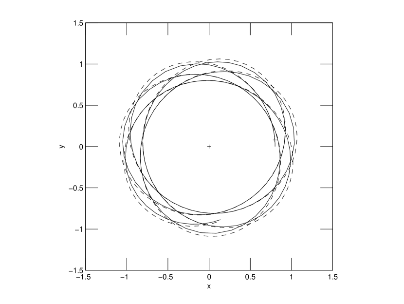
Figure 1: Sample x-y orbit in the logarithmic potential with energy/angular momentum constant $c=1.2$ and eccentricity $e=0.3$. The solid line is a numerical integration of the orbit, dashed line is a first-order p-ellipse approximation. See text for details. Note the end points of both in the lower right quadrant.

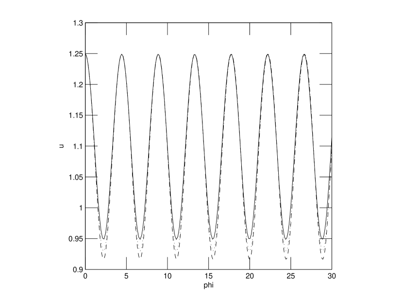
Figure 2: Inverse radius variable u versus azimuthal angle $\phi$ for a sample orbit in the logarithmic potential with energy/angular momentum constant $c=1.2$ and eccentricity $e=0.3$. The solid line is a numerical integration of the orbit, dashed line is the first-order p-ellipse approximation, and dotted line is the second-order approximation.

The approximate solution given by equation (10) is technically only good to first order in $e$, so we might expect it to have quite limited accuracy, except for very small values of $e$. However, Figures 1 and 2 compare the fit of equation (9) to a full numerical solution of equation (8) in the case of a moderate eccentricity of $e=0.3$. Figure 1 shows that the orbital fit is excellent over several orbital periods. Figure 2 shows that the approximation does not systematically drift away from the numerical solution after many cycles, and in fact is very close except near periapse. This shows that the approximate value of the precession factor $b$ is surprisingly accurate. (Part of the reason for this accuracy is the slow variation of the constant $c$ with eccentricity discussed above. These points will be discussed further below.)

3.2 Second Order Approximation (p-ellipse plus epicycle)

A clue to the lack of drift between the approximation (eq. (10)) and the solution noted in the last subsection is that the only second order terms that appear are proportional to $(ce^{2})\sin^{2}((1-b)\phi)$ and $(ce^{2})\cos^{2}((1-b)\phi)$. Moreover, there are no third or higher order terms. The fact that these are simple sine or cosine squared terms suggests that we could cancel them with more trigonometric functions in the approximate solution. Thus, we next consider approximations consisting of the sum of a p-ellipse and an elliptical epicycle (constant plus cosine term),

$$u=\frac{1}{p_{1}}\left[1+e\cos\left((1-b){\phi}\right)\right]^{1/2}+\frac{1}{p_{2}}\left[1+e_{2}\cos\left((1-b){\phi}\right)\right].$$ (12)

As before, we substitute this into equation (8) and equate the sum of terms with common powers of $e\cos((1-b)\phi)$ to zero. Additionally, we assume that $e_{2}\propto e$. We find that the resulting constant terms yield an expression for $c$, the first order terms yield the same value of $b$ as in the previous subsection, and the second order terms yield a relation between $e_{2}/e$ and $p_{2}/p_{1}$. If we further demand that equation (12) equals equation (10) at $\phi=0$ (and that both equal the initial value $u(0)$ of the full solution), then we obtain another relation between these two ratios and can solve for both. The results are,

$$c_{2}=\left(\frac{1}{p_{1}}+\frac{1}{p_{2}}\right)^{2}\left[1-\frac{e^{2}}{2p_{1}\left(\frac{1}{p_{1}}+\frac{1}{p_{2}}\right)}\right],\ b_{2}=1-\sqrt{2},\ e_{2}=\sqrt{1+e}-1,\ \mbox{and,}$$

$$\frac{a_{2}}{a_{1}}=\left(\frac{\frac{3}{4}-\frac{e_{2}}{e}}{2\left(\frac{e_{2}}{e}\right)^{2}}\right)\left[\left(\frac{3}{4}-\frac{e_{2}}{e}\right)^{2}+2\left(\frac{e_{2}}{e}\right)^{2}\right]^{1/2}.$$ (13)

The subscript “2” is used on the constants $b$ and $c$ to indicate that these values are accurate to order $e^{2}$.

It is assumed that the added cosine term has the same precession factor as the p-ellipse, so it does not drift from the p-ellipse approximation. A fortuitous cancellation leads to a zero second order correction to the precession factor $b$. We will see below that this is not generally true in other potentials.

This second order solution is plotted along with the numerical and first order solutions in the example of Figure 2, and we see that it doesn’t provide much improvement. The reason for this is that in going from the first to the second approximation, we have changed the higher order terms remaining in the orbit equation from two second order terms that partially cancel at most azimuths, to more than half a dozen third order terms, which do not generally cancel each other. Note that in this example: $p_{1}=1.93,p_{2}=1.73$, and $e_{2}=0.14$.

These third order terms have coefficients that are third order powers of sines and cosines, so they could presumably be eliminated by adding still more trigonometric terms to the approximate solution. We will not pursue the details, but it thus appears that we could improve the approximation with the addition of more epicycles or Fourier terms. Because the p-ellipse part of the solution is itself a good approximation, and because successive Fourier coefficients contain successively increasing powers of the p-eccentricity, the solution series should converge steadily for moderate eccentricities.

3.3 The Softened Logarithmic Potential

The accuracy of the simple p-ellipse approximate solution for orbits in the logarithmic potential is remarkable. In this and the following subsections we will see that it is not unique. On the contrary, it is useful over a range of interesting potentials. In this subsection we consider cases of equation (5) with $\delta=0$, but with nonzero core length $\epsilon$ (see eq. (1)), corresponding to the softened logarithmic potential.

In this case equation (5) can be written as,

$$uu^{\prime\prime}+u^{2}-c=-u^{2}(uu^{\prime\prime}+u^{2}),$$ (14)

where the left-hand-side is the same as equation (8), and the additional nonlinear terms have been placed on the right-hand-side. (Note that in this subsection we return temporarily to the convention of measuring all length units relative to $\epsilon$, i.e, here $u={\epsilon}/r$.) The term in parenthesis on the right-hand-side of equation (14) is also very similar to equation (8), which is a large part of the reason that the p-ellipse approximations continue to work well in this case.

Upon substitution for $u$ from equation (10), and equating zeroth and first order terms in $e\cos((1-b)\phi)$ as above (see Appendix A), we derive new forms for the factors $b$ and $c$ appropriate to this potential,

$$c_{1}=\frac{1}{p^{2}}\left(1+\frac{1}{p^{2}}\right),\ \ b_{1}=1-\left[2\left(\frac{1+\frac{2}{p^{2}}}{1+\frac{1}{p^{2}}}\right)\right]^{1/2}.$$ (15)

In the limit of orbit sizes much larger than the softening length ($p\gg 1$), these expressions reduce to those of equation (10), as they must. Additionally, in this case, we have two other limiting cases. The first is the limit of small orbit sizes where the rotation curve is linearly rising. In that case, $b_{1}\simeq-1$, which as we will shortly see is very interesting. The other special case is the exchange or rotation curve downturn region, defined by $p\simeq 1$, where there are also interesting resonances.

Before proceeding to discuss these cases it should pointed out that if we substitute the second order approximation of equation (12) into equation (14), we find that as in the previous subsection, there is no second order correction to the $b$ factor. The $c$ factor, however, does have a correction of order $e^{2}$,

$$c_{2}=\left(\frac{1}{p_{1}}+\frac{1}{p_{2}}\right)^{2}\left(1+\left(\frac{1}{p_{1}}+\frac{1}{p_{2}}\right)^{2}\right)\left[1+\frac{e^{2}(1-b)^{2}}{4p_{1}\left(\frac{1}{p_{1}}+\frac{1}{p_{2}}\right)}\right],$$

$$\ \ b_{2}=1-\left[2\left(\frac{1+2\left(\frac{1}{p_{1}}+\frac{1}{p_{2}}\right)^{2}}{1+\left(\frac{1}{p_{1}}+\frac{1}{p_{2}}\right)^{2}}\right)\right]^{1/2}.$$ (16)

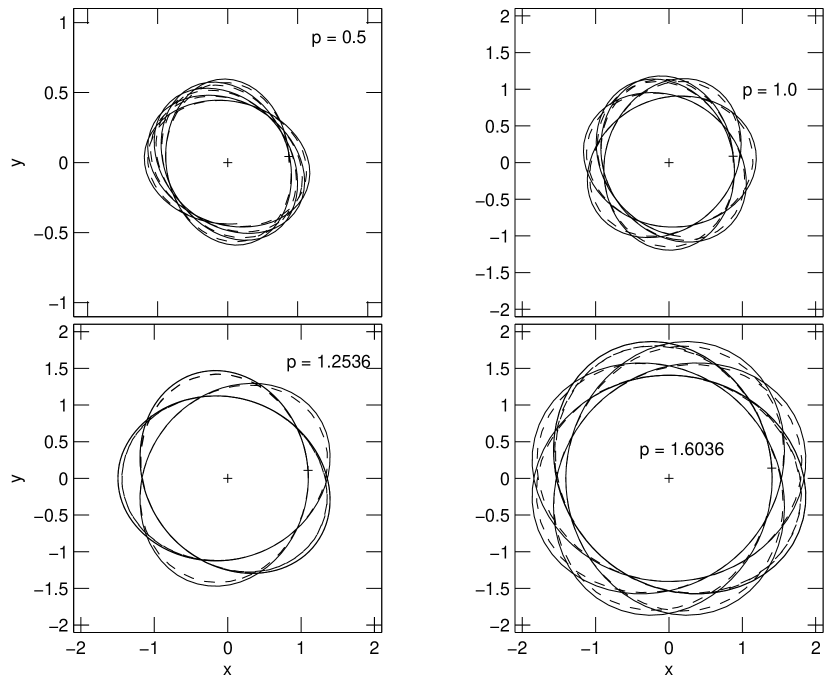
Figure 3: Four sample x-y orbits in the softened logarithmic potential with orbit sizes (semi-latus rectum) of $p=0.5,1.0,1.2536$ ($b=-2/3$), and $1.603567$ ($b=-3/5$). The p-ellipse eccentricity $e=0.3$ in all cases. The solid line is a numerical integration of the orbit, dashed line is the first-order p-ellipse approximation. Note scale difference in the upper left panel relative to the others. See text for details.

Figure 3 illustrates the goodness of fit of the (first order) p-ellipse solution, for different size orbits. As we would expect from the relation $b\simeq-1$, panel a) shows that the analytic solution is a slowly precessing, nearly closed, oval when $p$ is small (here $p=1/2$). The panel also shows that the analytic approximation fits the numerical solution quite well. It librates around it, but returns periodically, just as in the case of the pure logarithmic potential.

The second panel of Figure 3 is much like Figure 1, which corresponds to the large $p$ limit in the present case. That is, the solution is a more rapidly precessing, open p-ellipse, which the analytic approximation tracks quite well. It is interesting that we can see this behavior already at $p=1$, the case shown.

The third and fourth panels of Figure 3 show special cases of resonant orbits in the transition region. The third panel shows the case $b=-2/3$, corresponding to $p\simeq 1.2536$. Both analytic and numerical curves close (or nearly close) after 3 times around the center. The fourth panel shows the case $b=-3/5$, corresponding to $p\simeq 1.6036$, and we have more loops before closure.

The factor $b$ ranges over the interval $(-1,1-\sqrt{2})$. The infinite rational numbers in this interval correspond to closed (analytic) orbits. However, if we write a rational number m/n, there are very few in this interval with small values of m or n, i.e., low order period resonances. Like the above examples most of these will have radii of $p\simeq 1$. We reiterate that the value of $b$ does not depend on the eccentricity up to at least second order. The examples of Figure 3 have a moderate eccentricity of $e=0.3$.

In sum, Figure 3 shows that the first order p-ellipse approximation provides a good fit to orbits in this potential, as in the case of the logarithmic potential. In the previous subsection we found that the second order approximation yielded only a small improvement. In the present case the second order derivation involves a very unwieldy, high order polynomial in $p_{1}$ and $p_{2}$. Since this analysis produces no significant new results, I will not present it here (except for eq. (16)).

4 Potentials with Rising or Falling Rotation Curves

4.1 General p-ellipses

In the preceding section we considered the special cases of bound orbits in the logarithmic or softened logarithmic potentials, i.e., where $\delta=0$ in equation (5). In this section we consider positive and negative values of $\delta$, which correspond to falling and rising rotation curves. We will not, however, consider the most general form of equation (5). To simplify the analysis and the discussion, we will neglect softening and consider only pure power-law potentials. (We will also return to conventional variables, where $u=1/r$.)

In this case the equation of motion becomes,

$$uu^{\prime\prime}=cu^{2\delta}-u^{2}.$$ (17)

The simple p-ellipse solution in this case is,

$$u=\frac{1}{p}\left[1+e\cos\left((1-b){\phi}\right)\right]^{\frac{1}{2}+\delta},$$ (18)

with the variables defined as above. Specifically, we see that when $\delta=0$ we have the approximation of the previous section for the logarithmic potential, and when $\delta=1/2$ we have the ellipse for the Keplerian case. Given that in both of these cases equation (18) is an excellent approximation, it is not completely surprising that the equation is also an excellent approximation for all intermediate values of $\delta$. We will return to that point in a moment.

First we follow the procedure of the previous section. We substitute equation (18) into equation (17) and eliminate all terms of zeroth and first order in $e$, by making the identifications,

$$\ c_{1}=\left(\frac{1}{p}\right)^{2(1-\delta)},\ \mbox{and,}\ \ b_{1}=1-\sqrt{2(1-\delta)}.$$ (19)

Comparison to equation (10) shows great similarity, with the addition of some simple factors of $1-\delta$. The quantities $p$, $e$, and $\delta$ determine a p-ellipse, but it is also desireable to specify an orbit in terms of the conserved specific angular momentum and specific energy. Relations between these variables are presented in Appendix B.

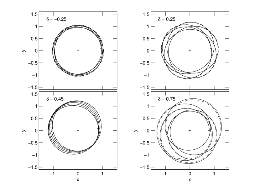
Figure 4: Four sample orbits in several power-law potentials with exponent $\delta$ values of $\delta=-0.25,0.25,0.45,0.75$. The p-ellipse eccentricity $e=0.2$ and orbit size $p=1$ in all cases. The solid line is a numerical integration of the orbit, dashed line is the first-order p-ellipse approximation.

In Figure 4 we show some sample approximate and numerically integrated orbits with a range of $\delta$ values, and with $p=1$, $e=0.2$ in all cases. A quick glance at this figure reveals a couple of basic points. First, the structure of comparable orbits varies a great deal over these different potentials. Second, the first order p-ellipse approximation is very good in all cases. If we look more closely at the individual panels we see that, as in the case of the logarithmic potential, the approximation librates a short distance from the numerical solution, only to return to it shortly thereafter. As we will discuss in the next section, this is generally true because the precession frequency implied by the second equality of (19) is exactly right for all the potentials (i.e., the same as in Newton’s theorem).

We see that the orbit shown in Figure 4b is similar to that of Figure 1. The exponent $\delta$ in this case is half way between that of the logarithmic and Keplerian potentials, so the fact that the orbit is similar to the former, but more slowly precessing, reflects continuity between these solutions. Figure 4c is very close to the Keplerian case, and the precession is very slow indeed. If we cross to the other side of the Kepler case, as in Figure 4d with $\delta=0.7$, both approximate and numerical solutions appear more erratic. This example is in the range between the Kepler solution and the Cotes spiral solution at $\delta=1.0$ in the present notation. (The MATLAB routine ODE45 was used throughout this paper.) In any case, we don’t expect the p-ellipse approximation to be very useful for values of $\delta$ of about or greater than 1.0.

Figure 4a shows an example of going past the logarithmic potential to those with negative values of $\delta$. The exponent $1/2+\delta$ of equation (18) becomes very small in the vicinity of $\delta=-1/2$, so even with significant values of the eccentricity $e$, the radial excursion of orbits is very small. Nonetheless, the figure shows that the p-ellipse approximation continues to be good.

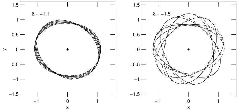
Figure 5: Two sample orbits in power-law potentials with steeply rising rotation curves, i.e., exponent $\delta$ values of $\delta=-1.1,-1.5$. The p-ellipse eccentricity $e=0.2$ and orbit size $p=1$ as in the previous figure. The solid line is a numerical integration of the orbit, dashed line is the first-order p-ellipse approximation.

The two panels of Figure 5 show sample orbits at still more negative values of $\delta$. The first panel shows a cases where $\delta=-1.1$ is very close to that of the solid-body potential, and so is quite similar to Figure 3a. The second panel shows a still more extreme case ($\delta=-1.5$), and here the deviations between approximate and numerical orbits become quite significant. Thus, it seems that the p-ellipse approximation is at best only qualitatively useful for values of $\delta$ much more negative than the solid-body case.

The normalized (by a factor of $p^{2}$) second order terms that remain when the p-ellipse is substituted into the equation of motion provide an estimate of the inaccuracy of that approximate solution. Technically, they provide an estimate of the inaccuracy of the $u^{\prime\prime}/u$ value, but given the common periodicity of $u$ and its derivatives, this is roughly equivalent to the relative inaccuracy in $u$. All the second order terms are proportional to $(e\cos((1-b)\phi))^{2}$. If we take the average value of 1/2 for the cosine term, a first rough estimate of the error is $e^{2}/2$, which, when compared to the numerical results, turns out to be about right in the vicinity of $\delta=0$.

The $\delta$ dependence of this error estimate is given by the function: $(1+2\delta)(1-\delta)(\delta^{3}+0.5\delta^{2}+3.5\delta-1)$. When $\delta$ values vary from -0.5 to 0.5, the absolute values of the function are always less than 1.2, and mostly in the range 0.5-1.2, i.e., of order unity. For values $\delta\ll-0.5$, the absolute value of the function rises rapidly (eventually as $(1+2\delta)\delta^{4})$, explaining the diminished accuracy of the p-ellipse approximation. Within the domain of $\delta$ values of the most interest (-0.5 to 0.5), eccentricity is the dominant factor in the error estimate. Section 5.2 offers a way to derive more accurate p-ellipse approximations at large eccentricity.

The approximate nature of the first order p-ellipses, and these limitations on their domain of accurate application, distinguish them from a universal analytic solution. However, the latter evidently doesn’t exist, and the p-ellipses provide accurate orbit approximations in power-law potentials over most of the domain of interest for studies of galaxy dynamics.

4.2 Second Order Approximation for Power-Law Potentials

As in the case of the logarithmic potential, we can attempt to eliminate terms of second order in $e$ by adding the $p_{2},e_{2}$ terms of equation (12) to equation (18). In the more general cases of $\delta\neq 0.0$ there are more second order terms than in the logarithmic potential, so we might expect the correction to be more useful than in that case.

However, direct comparison of the second order approximation to numerical integrations in cases like those shown in Figures 4 and 5 shows that the situation is not that simple. I find that for $\delta$ values in the range $0<\delta<1/2$ there is little difference between the p-ellipse and second order approximations, as in the case of the logarithmic potential. For $-1/2<\delta<0$, the second order approximation fits the numerical orbits significantly better than the first order p-ellipse. For $\delta<-1/2$, the amplitude of the second order approximation fits better, but its precession rate is apparently not accurate because the orbital phase drifts quite rapidly. We conclude that, as in the case of the logarithmic potential, there is not much reason to prefer the second order approximation in the case of general power-law potentials.

The following equations define the second order solution,

$$b_{2}=1-\left[\frac{2(1-\delta)}{1+\frac{\delta}{2}\left(1-4{\delta}^{2}\right)\left(\frac{p_{2}}{p_{1}+p_{2}}\right)e^{2}}\right]^{1/2},$$

$$e_{2}=\left(1+e\right)^{\frac{1}{2}+\delta}-1,\ \ \ (initial\ condition),$$

$$\frac{p_{1}}{p_{2}}=\left(\frac{(1+2\delta)\left(\frac{3}{4}-\frac{e_{2}}{e}\right)}{2\left(\frac{e_{2}}{e}\right)^{2}}\right)\left[1\pm(1+2\delta)\left[\left(\frac{3}{4}-\frac{e_{2}}{e}\right)^{2}+2(1-2\delta)\right]^{\frac{1}{2}}\right],$$

$$p_{1}=\left(1+\frac{p_{1}}{p_{2}}\right)c^{\frac{-1}{2(1-\delta)}},$$ (20)

where the variables $e,c,$ and $\delta$ are given, and the above equations are solved for $p_{1},p_{2},e_{2}$, and $b_{2}$. The equation labelled $initial\ condition$ is derived by equating the initial value of the first and second order approximations.

The expression for $b_{2}$ in equation (20) has a slight dependence on $e$. This allows the second order approximation to drift relative to the first order solution. It also allows for the possibility of a rational value of the precession period relative to the orbital period, and closed orbits, at special values of $e$. We will consider this further in Sec. 5.

4.3 Potentials with Closed Orbits

The second equality of (19) allows for values of $\delta$ that yield rational values of $b_{1}$, and thus, closed orbits for all low-to-moderate values of $e$ in those potentials, in the first order p-ellipse approximation. These potentials are generally isolated, i.e., not dense in the mathematical sense, on the $\delta$ axis, though there are exceptions. The existence of these closed orbits and their basic structure can also be deduced from the apsidal precession theorem and its generalizations. However, there is the question of how small the eccentricity must be for Newton’s theorem to be valid, and the generalizations of Valluri et al. (2005) to high eccentricities are complex. If p-ellipse formulae like those of eqs. (19) and (20) are sufficiently accurate, then they provide simple alternatives for guidance on these questions. We examine this question in this subsection.

From the second equality of (19) we deduce that in order for $b_{1}$ to have a rational value, we must have,

$$\delta=1-\frac{1}{2}\frac{j^{2}}{k^{2}},$$ (21)

where $j$ and $k$ are integers. Then, $b_{1}=(k-j)/k$. As a simple and generalizable example consider the sequence $k$ = 1, 2, 3,…, with $j=k+1$. The corresponding sequence of $b_{1}$ values is $b_{1}=-1/k$. Table 1 gives $\delta$ values for some elements of this sequence.

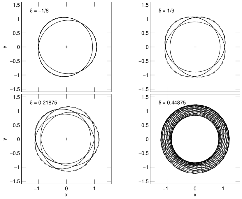
Figure 6: Four sample closed orbits in power-law potentials with exponent $\delta$ values of $\delta=-1/8,1/9,7/32,0.44875$. The p-ellipse eccentricity $e=0.2$ and orbit size $p=1$ in all cases. The solid line is a numerical integration of the orbit, dashed line is the first-order p-ellipse approximation. In the lower right panel only the numerical curve is shown for clarity, though the approximation agrees as well as in the other cases.

Figure 6 gives examples of orbits in this sequence with eccentricities of $e=0.2$ and orbit sizes of $p=1.0$. Specifically, the $k$ = 2, 3, 4, and 20 orbits are shown. The first panel shows a very simple closed orbit, that with $\delta=-1/8$ is close to the logarithmic potential. The analytic and numerical solutions are very similar to each other. To keep the plot readable we only show a couple of times around the orbit. However, a plot like that of Figure 2 for many orbits shows no drift between the numerical and analytic curves. I will not attempt to prove that the orbits in this potential are closed, but it appears that for practical purposes they are. (This has been checked at other values of $e$ as well.)

The second panel of Figure 6 corresponds to a slightly falling instead of a rising rotation curve with $\delta=1/9$. It is slightly more complex, but still closed, and with excellent agreement between the analytic and numeric curves. As before, there is no drift between the two curves after many orbits.

The trends of more complexity in the closed curves, and good agreement between analytic and numeric curves, continue in the third panel of Figure 6, where $\delta=7/32$.

The fourth panel, where $\delta\simeq 0.45$, shows that things get very interesting as we approach the Kepler case. The orbits become very slowly precessing p-ellipses that eventually close. As k advances to large values in this sequence, $b_{1}$ goes to zero, and according to equation (21) $\delta$ goes to 1/2. Thus, the sequence converges on the Kepler case. In contrast to the sparsity of potentials in this sequence in the region of the logarithmic potential, the convergence of this sequence shows that such potentials do densely populate the $\delta$ axis at values just less than the Kepler value. These statements are also true for a second sequence defined by $k$ = 1, 2, 3,…, with $j=k+2$, and so on.

Thus, the properties of the p-ellipses, originally derived as simple analytic approximations, have revealed families of potentials with (at least practically) closed orbits, like the Kepler potential, and unlike the logarithmic potential. Appropriately, these families cluster thickly on one side of the Kepler potential. Interestingly, these special potentials include the $\delta=-1/8$ and $1/9$ potentials, but not the simple $\delta=1/8$ and $1/4$ potentials. This is explained by the precession law of the p-ellipses.

I have avoided discussing the very simple case of $k=1$, $j=2$, and $b_{1}=\delta=-1$. This is the first element of the sample sequence above, and is the solid-body potential. The analytic and numeric curves for this highly resonant case do not agree. This is true in spite the fact that we have shown good agreement in examples above, which have $\delta$ values a little less than -1.0.

5 Discussion and Applications

5.1 Apsidal Precession and Integrals of the Motion

It has been noted already that one of the secrets of the success of the first-order p-ellipse approximations is that their precession rates accurately match those of the true orbits in power-law potentials up to moderate eccentricity values. It remains to demonstrate explicitly that they satisfy Newton’s apsidal precession theorem, and consider large eccentricities.

As to the former, we note that the minimum of u (apoapse) occurs when $(1-b)\phi=\pi$, the maximum (periapse) when $(1-b)\phi=0$, and the difference is,

$$\Delta\phi=\frac{\pi}{\sqrt{2(1-\delta)}},$$ (22)

which is the apsidal precession theorem for p-ellipses. Valluri et al. (2005) remind us that with an acceleration proportional to $1/r^{N-3}$, Newton’s apsidal precession theorem gives $\Delta\phi=\pi/\sqrt{N}$. When we compare this form of the acceleration to the one used in this paper (with no softening), we find $N=2(1-\delta)$, so the two expressions for the apsidal precession are the same. This proves the that the first-order p-ellipses satisfy the apsidal precession theorem. (Note that with eq. (15) we also can readily derive the apsidal precession as a function of orbit size in the softened logarithmic potential.)

Valluri et al. (2005) emphasized that apsidal precession depends on orbital eccentricity at large eccentricities, so the Newton formula and equation (22) are not correct in that limit. These authors derived integral expressions for the dependence of the precession rate on N and $e$ for the power law potentials. The first equation of (20) provides a simple approximate formula for this dependence.

Before comparing this simple formula to the Valluri et al. results, we should recall that the p-ellipse eccentricity we have used up to this point is not the same as the usual definition of the eccentricity (except in the case of the inverse square law). If an orbit is assumed to be approximately a precessing ellipse, then one definition of eccentricity is in terms of the periapse distance using the formula $r_{min}=a(1-e)$. We will call the eccentricity defined in this way the classical eccentricity, and denote it $e_{o}$. The classical eccentricity and the p-ellipse eccentricity used above are related by the equation,

$$\left(1-e\right)^{\delta+\frac{1}{2}}=1-e_{o}.$$ (23)

The classical eccentricity is generally significantly less than the p-ellipse eccentricity, though they are nearly the same for potentials close to the Kepler potential.

With that notational disparity accounted for, we return to the topic of the dependence of precession on eccentricity, and the comparison of Valluri et al.’s results to the $b_{2}$ expression in equation (20). First of all, it should be emphasized that we have seen that the second-order approximation described above was not found to be highly accurate in many cases. Valluri et al.’s semi-analytic apsidal precession angles, illustrated in their Figure 2, are more accurate than those derived from equation (20).

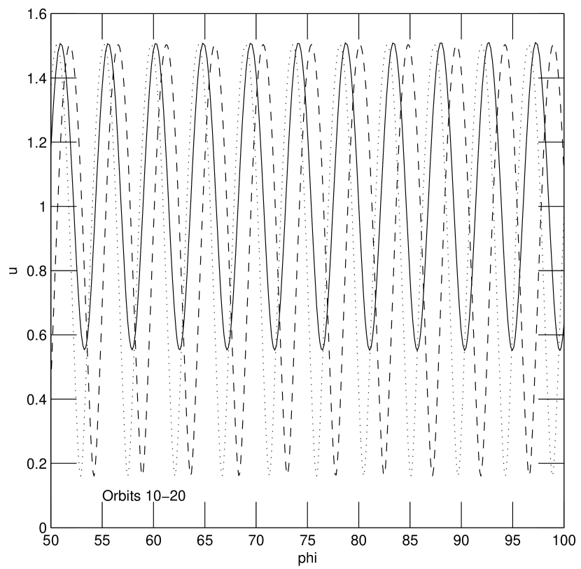
Figure 7: Inverse radius variable u versus azimuthal angle $\phi$ for a sample orbit in the $\delta=1/9$ potential with energy/angular momentum constant $c=1.0$ and eccentricity $e=0.95$. The solid line is a numerical integration of the orbit, dashed line is the first-order p-ellipse approximation, and dotted line is the second-order approximation.

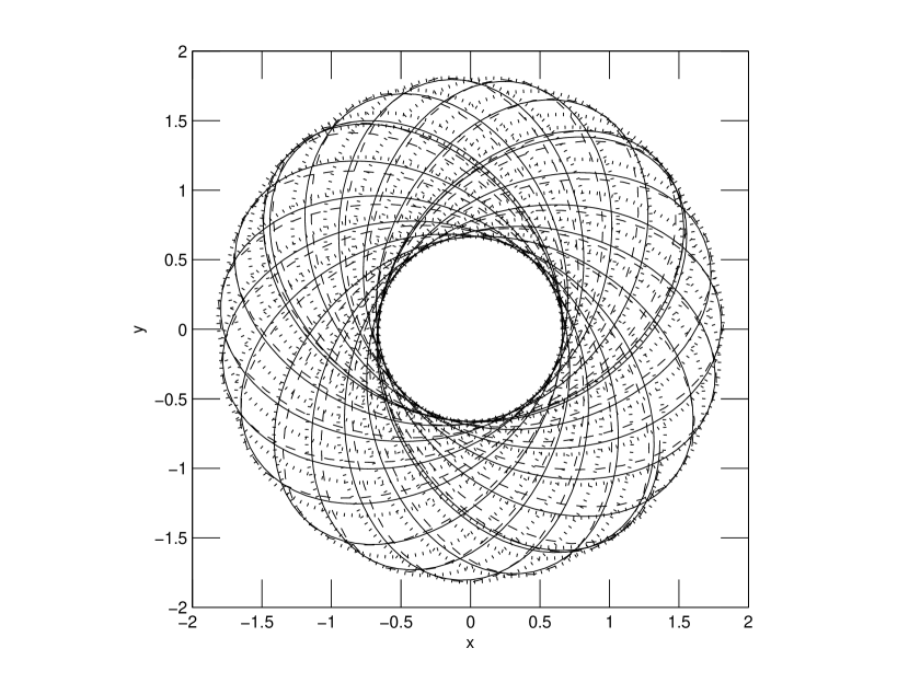
Figure 8: Sample x-y orbit in the $\delta=1/9$ potential with energy/angular momentum constant $c=1.0$ and eccentricity $e=0.95$. The solid curve is a numerical integration of the orbit, dashed curve is the first-order p-ellipse approximation, and dotted curve is a spirographic approximation as described in the text.

Nonetheless, the $u-\phi$ plot in Figure 7 shows an example where the precession of a numerical orbit solution after 10-20 orbits is much better fit by the second order precession rate than the first order rate. (Their libration amplitudes are comparable.) Equation (20) does seem to be an improvement over the $b_{1}$ formula of equation (19). The example shown in Figure 7 has $e=0.95$ and $e_{o}=0.84$, so it is quite eccentric. The example in Figure 7 has $\delta=1/9$, a closed orbit value, but at this large eccentricity the orbits are not closed (see Fig. 8).

The $b_{2}$ expression of (20) also captures and helps us to understand many of the qualitative features of Valluri et al.’s results. First of all, the dependence on eccentricity is quite weak in equation (20), and so, it only becomes important for large values of $e$ (unless $\delta$ is very large). Indeed, either equation (20) or Valluri et al.’s graphs show how good an approximation the constant precession rate $b_{1}$ is for given values of $e$ and $\delta$ (and thus overcome the primary objection to the use of the apsidal precession theorem up to modest eccentricities). Secondly, both formulations predict that the precession rate is constant at all eccentricities for the logarithmic potential. Thirdly, they both agree that the apsidal angle $\Delta\phi$ increases (decreases) with eccentricity when $\delta<0$ ($\delta>0$). In fact, equation (20) provides a fair quantitative approximation to the plots of Valluri et al. at values of $\delta$ not far from zero.

Valluri et al. also state that their work gave no evidence for “isolated cases of zero precession as e was increased.” The $b_{2}$ expression in (20) indicates that such cases might exist at values of $\delta$ just slightly less than 1/2, but even if this prediction is confirmed, these cases would be very anomalous. Another somewhat arcane prediction of equation (20) and Valluri et al.’s results is that potentials very near the resonant ones discussed in the previous section should have a closed orbit at one specific, high value of the eccentricity. These potentials have smaller values of $\delta$ than the resonant one for positive $\delta$.

The discussion of this subsection clearly relates to the classical integrals of the motion. The precession rate $b$ (or the precession frequency divided by the orbital frequency), is an integral of the motion, much like the initial orbital phase angle which is often used as such (see Sec. 3.1 of Binney & Tremaine 1987). By indicating the presence of closed orbits, the expressions for $b$ in (19) and (20) tell us (approximately) when these integrals are isolating.

5.2 An Alternate Approach to p-ellipse Orbit Approximation

5.2.1 Better Approximations at Larger Eccentricities

The p-ellipse orbit approximations above were derived from an analytic perturbation analysis, with some implicit constraints. In this section we learn more about these approximations by relaxing some of these constraints. Figure 7 shows how, in the case of an orbit of high eccentricity ($\delta=1/9$ and $e=0.95$), the p-ellipse approximations drift in period relative to the numerical solution. (This is not surprising given the Valluri et al. (2005) results on apsidal precession.) This motivates an attempt to improve the p-ellipse solution by changing the value of $b$ to match the numerical result. In the case shown in Figure 7 this means changing from the analytic value of $b_{2}=-0.3027$ to -0.3558.

According to equation (19) or (20), a different $b$ factor corresponds to a different $\delta$ value. In this case (using eq. (19)), we go from $\delta=1/9=0.1111...$ to $\delta^{\prime}\simeq 0.0809$. Another difficiency of the p-ellipse approximation shown in Figure 7 is the radial range. With the revised value of $\delta$ we can also revise $p$ and $e$ to fit the numerical maximum and minimum radius. The revised p-ellipse approximation is given by the equation,

$$\frac{1}{r}=1.1105\left[1+0.7026\cos(1.3558{\phi})\right]^{0.5809}.$$ (24)

This provides a very good fit to the orbit as shown in Figure 8, where the numerical orbit is shown by the solid line, and the approximation by the dashed line.

To recapitulate, we have treated the p-ellipse quantities as free parameters, first adjusting the precession rate to match the numerical value, and then the orbital size and eccentricity to match the radial range. The $\delta$ value was also changed to maintain the relationship of equation (19). This procedure seems to yield an highly accurate orbit approximation for such loop type orbits, even at quite high eccentricity.

5.2.2 p-ellipse Transformation and Perturbation Approximation

The result of the previous subsection can be viewed as achieving a more accurate fit to a high eccentricity orbit than the first-order p-ellipse by using a smaller eccentricity p-ellipse orbit taken from a different (power-law) potential. This suggests that there is an approximate mapping between p-ellipses, representing an approximate symmetry of the power-law potentials. The nature of this relation is that the orbits in a given potential at high eccentricity correspond to orbits of lower eccentricity in a different potential, with the same precession rate. Of course, the first-order p-ellipse approximation fits the lower eccentricity orbit better.

As an aside, note that this relation suggests that periodic orbits may be found at high eccentricity in a potential with generally aperiodic orbits, when the correspondence is to an individual orbit in a periodic potential.

However, the assumption that the first order equation (19) holds at high eccentricity is likely to be a rather crude ansatz. Another approach is to return to the perturbation analysis of Sec. 4.1, but now allow the $\delta$ factor of the p-ellipse approximate solution to be different than that of the equation of motion, call it $\tilde{\delta}$. We will still fix the $b$ factor to the numerical result, because even a small precessional drift will result in a large difference between the approximate and true orbit.

Then, requiring the cancellation of zeroth and first order terms in $e\cos((1-b)\phi)$ yields the following relation,

$$(1-b)^{2}=\frac{2(1-\delta)}{\left[1-\frac{\delta}{2}(1-4\tilde{\delta}^{2})e^{2}\right]},$$ (25)

(Note the similarity to the expression for $b_{2}$ in eq. (20))

For a given potential exponent $\delta$ and precession parameter $b$, this gives a relation between the exponent $\tilde{\delta}$ of the corresponding potential, and the eccentricity of the p-ellipse in that potential. Requiring that the approxmation also fit the maximum and minimum radii of the numerical orbit (which can be derived from the conserved energy and angular momentum, see Appendix B) gives three relations for the variables $\tilde{\delta}$, $e$, and $p$. Second order terms in the perturbation expansion do not cancel, but since the $b$ value is correct, this procedure is better than the direct second-order approximation. The results for the case shown in Figure 8 are: $\tilde{\delta}=-0.003$, $p=0.87$, and $e=0.77$. The values are very similar to those of equation (24). This perturbation approach is less ad hoc than that used to derive equation (24), and thus, provides a more solid basis for approximating high eccentricity orbits.

5.2.3 Epicycloid Comparison

A specific comparison to the epicycloid approximation of Adams & Block (2005, see their eqs. (20) and (21)) is also shown in Figure 8, as a dotted curve. This curve was constructed by requiring that it have the same maximum and minimum radii, and the same precession rate as the numerical solution. It can be seen from Figure 8, and the corresponding $u-\phi$ graph that it deviates from the numerical solution a bit more at intermediate radii than the specially fitted p-ellipse.

Overall, the simple versions of both approximations seem to be about comparably accurate in the case shown. It seems likely that the epicycloids, like the p-ellipses, can provide good orbit approximations in the potentials studied above. Adams & Block (2005) have considered the properties of the epicycloid orbits in general potentials, so I will not examine this issue in detail in this paper. The advantages of the p-ellipses include their simple form in polar coordinates, and the fact that their orbit parameters change in very simple ways as functions of the conserved quantities and the parameter $\delta$ in power-law potentials.

5.3 Galaxy Collisions, Bars and Precession Period Resonance

In this paper, I will not present any detailed applications of the p-ellipse theory developed above. Indeed, since the orbits have long been studied numerically in many relevant cases we do not expect new applications, as much as new perspectives on old applications. Nonetheless, in this section I will highlight a couple of applications that seem worthy of further development.

The first is simply the application of p-ellipses to obtain the general characteristics of satellite orbits in potentials with either rising or falling rotation curves. The simplicity of p-ellipse allows one to quickly produce a wide range of possible satellite orbits in any particular situation. In studies of interacting galaxies, one can then use the impulse approximation to estimate the effect of a close encounter on initially circular stellar orbits in the disk of the primary. The initial effects of such encounters are kinematic, with self-gravitational effects taking time to accumulate, so solutions of the perturbed orbit equations would provide a reasonable picture of the early development of tidal structures (see review of Struck 1999). This, in turn, would be a very efficient means of constraining the satellite orbit and the primary gravitational potential needed to produce observed tidal features, at least in encounters with modest dynamical friction.

The second is based on the slowly precessing orbits in the inner regions of the softened logarithmic potential discussed in Sec. 3.3 and illustrated in Figure 3a. Equation (15) tells us how the precession $b$ depends on orbit size $p$ in this case. In particular, for values of $p<1$, we have $b_{1}\simeq-1$, which is the slow precession. If a disturbance (e.g., tidal) elongates initially circular orbits in this region, the slow precession tells us that they will stay approximately aligned for some time. This in itself is not remarkable in a potential that is approximately solid-body in that region. However, the p-ellipse equations not only tell us about this kinematic bar, but they also tell us quantitatively how this structure would precess into a spiral at somewhat larger radii. Of course they do not include the effects of self-gravity on these kinematic waves.

A third application concerns resonant orbit-satellite interactions. Tremaine & Weinberg (1984), for example, have emphasized the importance of resonant orbits in galaxy bar dynamics and in dynamical friction effects on satellites. Frequently, when resonances are discussed in galaxy dynamics they are Lindblad resonances. These are local (in radius), and usually visualized in the epicyclic approximation as small integer ratios between the epicyclic period and the period of the mean (guiding center) orbit.

The existence of closed orbits and nearly closed orbits described above naturally raises the topic of resonant interactions in galaxy disks involving these orbits. One example would be resonances between eccentric p-ellipse type orbits and circular orbits with resonant periods, and radii close to the apsides of the eccentric orbit. Because of the radial range of the eccentric orbit, such interactions would not be as localized as the Lindblad resonances. For non-Keplerian potentials, Kepler’s third law generally has a (complicated) dependence on eccentricity (see Appendix C), which will make the cataloguing of such resonances somewhat difficult. These resonances seem qualitatively similar to those between orbit families in barred potentials, so like the latter they may play a role in building bulges, especially at early times.

Period resonances involving the precession of p-ellipse orbits may also be important. Figures 6a,b remind us that potentials close to the logarithmic potential with such orbits have precession periods of about a few times the orbital period. In these nearly flat rotation curve potentials, this means that the precession periods of disk stars are about equal to the orbital periods of satellites with orbital radii a few times larger. Higher order resonances would occur at larger satellite orbital radii. Thus, especially in the early stages of galaxy evolution, this interaction could play a very important role in the evolution of disks and satellite orbits. It may also be important in galaxy interactions. The immediate objection is that the closed orbit potentials described above are very sparsely distributed on the $\delta$ axis, i.e., very rare. A counter-argument is that potentials with orbits that are nearly closed, i.e., do not drift much in phase over a duration of several precession periods, span finite intervals on the $\delta$ axis near the closed orbit potentials.

Resonant orbit-precession interactions might also be important between forming planets in accretion disks if the disk mass is great enough to modify the Kepler potential, as seen by planets on elliptical-like orbits. As described above, there are many closed orbit potentials with $\delta$ slightly greater than the Kepler value of 1/2. The precession rate is slow for these potentials, but the evolutionary times extend over at least thousands of orbital periods, so this is not a problem.

A similar application may be found for the orbits of stars in dense clusters around massive black holes in galaxy nuclei. If the central black hole dominates, but the distributed mass of the star cluster is non-negligible, the effective potential will have a rotation curve that is slightly flatter than a Keplerian one. This is again in the region of dense closed orbit potentials, so precessional resonance interactions with satellite star clusters or other massive black holes may be important. As usual with resonant interactions, they likely involve only a small minority of stars, and so, specially designed N-body simulations are needed to study the phenomenon.

6 Summary and Conclusions

In the sections above, we have shown that curves derived as powers of ellipse functions, called p-ellipses, provide simple, yet surprisingly accurate approximations to orbits in a range of power-law potentials, including the well-known logarithmic potential, and softened power-law potentials. For a given power-law potential the p-ellipse function is nearly as simple as an ellipse, but the family of p-ellipses extends continuously across a physically interesting range of potentials.

There are at least two reasons why p-ellipses are good orbital approximates across this range of potentials, and are likely to be the best simple, analytic functions to do so. First, p-ellipses match the tendency for orbits of a given energy and angular momentum to become more circular as the potential changes from Keplerian to solid-body (and $\delta$ decreases). In this sense the p-ellipses adjust well to the appropriate orbital shape in a given potential. Secondly, the precession rate obtained by demanding that the p-ellipse satisfy the equation of motion in a given potential to first order in eccentricity is the identical to that given by Newton’s theorem. Thus, the p-ellipses precess correctly. Moreover, a second order approximation yields an eccentricity dependence of the precession rate that is in qualitative agreement with the Valluri et al. (2005) semi-analytic results.

A number of the results obtained above for p-ellipses, like the apsidal precession rates in power-law potentials, are not new, and good approximations to individual orbits can be obtained with epicycles or numerical integration. However, a family of simple curves like the p-ellipses allow us to readily see trends across a range of potentials, so they provide a simple, conceptual picture for orbital variations, as discussed in the introduction.

Moreover, as shown in the previous sections the p-ellipses provide a very powerful tool for studying characteristics like the occurrence of (non-circular) closed orbits as a function of eccentricity in different potentials. The key feature of the p-ellipses in this regard is a relatively simple approximate formulae for precession rates as a function of $\delta$ and $e$. Newton’s theorem is valid in the limit of small eccentricity, and Valluri et al.’s extensions involve integrals that must be evaluated numerically. Equations (19) and (20), though approximate, offer convenience. (Also see eq. (25).)

The example of the softened power-law potentials holds out the hope that the p-ellipses can provide useful orbit approximations in other non-power-law potentials. Non-axisymmetric potentials have not been considered in this paper, but it seems reasonable to hope that p-ellipses could provide good approximations to loop orbits in such potentials. This issue deserves more study.

In Section 5.3 I described several examples of how the systematics of p-ellipses might shed light on important astrophysical problems. This conclusion will be even more general if p-ellipses prove to be good orbital approximations in more types of potential.

Orbit theory is more general than celestial mechanics, and the p-ellipse approximations should also be relevant to any field than involves orbits in general potentials. Electron orbits in general, steady (gradient) electric and magnetic fields are obvious examples.

In sum, there seems to be room for a great deal more development of the theory and application of these simple curves. Their simplicity may allow us to address a number of complex issues that would be hard to study directly through the accumulation of numerical examples.

Appendix A Some Perturbation Analysis Details

The purpose of this brief appendix is to provide a few more details, and a slight extension of the perturbation analysis leading to the results of equation (10). This is the simplest of several such calculations in the main text, but is representative of the common procedure.

That procedure consists of substituting the adopted solution (first equality of eq. (10)) into the equation of motion (8), and gathering terms of common order in the factor $e\cos((1-b)\phi)$. Then the requirement that these terms cancel up to a given order is used to derive relations between the paramenters. In this case, the zeroth order terms yield the condition,

$$c=\frac{1}{p^{2}}\left(1-\frac{(1-b)^{2}e^{2}}{4}\right),$$ (A1)

for the constant $c$ of equation (8) in terms of the variables $b$, $p$, and $e$. Note that since this is an expansion in terms of $e\cos((1-b)\phi)$, the $e^{2}$ term (with no cosine factor) is included in the zeroth or constant condition. This factor is not included in the (first-order) results given in equation (10).

Terms of first order in $e\cos((1-b)\phi)$ yield the condition,

$$\frac{1}{2}(1-b)^{2}-2+cp^{2}=0,$$ (A2)

which, in combination with the previous condition, yield an expression for the $b$ factor.

The terms of second order in $e\cos((1-b)\phi)$ are,

$$1-\frac{(1-b)^{2}}{4}=\frac{1}{2}-\frac{e^{2}}{4},$$ (A3)

where a common factor of $1/p^{2}$ has been dropped, and the result for $(1-b)$ from the previous condition has been used. With no extra parameter to adjust, these terms do not cancel, but do provide an estimate of the p-ellipse accuracy. It is interesting that while all second order terms are small at small eccentricity, the term above is smallest at large eccentricity. This is not the case for other power-law potentials.

Appendix B Relations Between Orbital Parameters

In this appendix I present some relations between orbital parameters, especially those between the semi-major axis $a$, the eccentricity parameter $e$, and the specific angular momentum $h$ and specific energy $\mathcal{E}$. The relation between $h$ and the constant $c$ is given in equation (4), and equation (19) relates the latter to the semi-latus rectum $p$, for a first-order p-ellipse. Combining these yields,

$$\frac{h^{2}}{GM_{*}}=p^{2(1-\delta)}=\left(\frac{a}{g_{o}(e)}\right)^{2(1-\delta)},$$ (B1)

$$\mbox{with,}\ g_{o}(e)=\frac{1}{2}\left[\frac{(1-e)^{1/2+\delta}+(1+e)^{1/2+\delta}}{(1-e^{2})^{1/2+\delta}}\right].$$ (B2)

The second equality in (B1), $h$ versus $a$, is derived from a generalization of equation (11) for the case $\delta\neq 0$.

The specific energy is defined as,

$$\mathcal{E}=\frac{1}{2}\left(v^{2}-\frac{GM_{*}}{\delta r^{2\delta}}\right),\ \mbox{for}\ \delta\neq 0,$$ (B3)

$$\mbox{and,}\ \mathcal{E}=\frac{1}{2}\left(v^{2}-GM_{*}\ln(r)\right),\ \mbox{for}\ \delta=0,$$ (B4)

where $v$ is the total relative velocity of satellite. The radial velocity, $v_{r}$, can be derived in terms of the azimuthal velocity by differentiating equation (18) with respect to time. Then, the azimuthal velocity can be eliminated using the relation $h=rv_{\phi}$. After some simplification, for the case with $\delta\neq 0$, we get,

$$\mathcal{E}=\frac{GM_{*}}{2a^{2\delta}}\ g_{\mathcal{E}}(e,\delta),$$ (B5)

$$\mbox{with,}\ \ g_{\mathcal{E}}(e,\delta)=g_{o}^{2\delta}(1+e)^{1+2\delta}\left[1-\frac{1}{\delta}(1+e)^{(\delta-1)(1+2\delta)}\right].$$ (B6)

For the case $\delta=1/2$, equations (A1), (A2), (A5), and (A6) reduce to the usual Keplerian elliptical orbit relations: $\mathcal{E}=-GM/2a$ and $h^{2}=GMa(1-e^{2})$.

For the case $0<\delta\ll 1/2$ (i.e., nearly flat, but slightly decreasing rotation curve), we have,

$$g_{o}\simeq\frac{1}{1-e_{o}},\ g_{\mathcal{E}}\simeq 1+e-\frac{1}{\delta}\simeq-\frac{1}{\delta},$$ (B7)

$$h^{2}=GM_{*}a^{2}(1-e_{o})^{2},\ \mbox{and},\ \mathcal{E}=\frac{-GM_{*}}{2\delta a^{2\delta}},$$ (B8)

where $e_{o}$ is the “classical” eccentricity of equation (23). In contrast to the full relations, these limiting cases can be easily inverted to derive $a,e$ as functions of $h,\mathcal{E}$.

Appendix C Time-Azimuth Relations and Kepler’s Law for p-ellipses in Power-Law Potentials

Relations between time and azimuth for p-ellipse orbits in power-law potentials are not treated in the main text. Since these relations are likely to be very important for any application involving p-ellipses we derive them here. Specifically, we can derive an invertible analytic expression for the logarithmic potential, and a implicit relation for potentials with small values of $\delta$. To begin, the equation for the conserved specific angular momentum gives the azimuthal frequency, $d\phi/dt=h/r^{2}$. Next, we substitute the p-ellipse solution for r to get,

$$\frac{d\phi}{dt}=\frac{h}{p^{2}}\left[1+e\cos\left((1-b)\phi\right)\right]^{1+2\delta}.$$ (C1)

In the case of the logarithmic potential, $\delta=0$, this can be integrated to obtain,

$$\frac{h(1-b)t}{2p^{2}}\sqrt{1-e^{2}}=\tan^{-1}\left\{\sqrt{\frac{1-e}{1+e}}\left[\tan\left(\frac{(1-b)\phi}{2}\right)-\tan\left(\frac{(1-b)\phi_{o}}{2}\right)\right]\right\},$$ (C2)

where, on the right hand side, we assume that there is an initial azimuth, $\phi_{o}$, on the left we assume that the initial time is $t=0$.

By setting $(1-b)\phi=2\pi$ and $\phi_{o}=0$ we get an expression for the orbital period, $T$, in the logarithmic potential,

$$T=\frac{p^{2}}{h(1-b)}\ \frac{2\pi}{\sqrt{1-e^{2}}}.$$ (C3)

Using equations (10) for $b$, (11) for $p$ in terms of the semi-major axis $a$, and (B1), (B2) for $h$ (with $\delta=0$), we derive Kepler’s third law for first order p-ellipse orbits in the logarithmic potential,

$$T^{2}=\frac{2\pi^{2}}{GM_{*}}\left[\frac{2}{\left(\sqrt{1+e}+\sqrt{1-e}\right)^{3}}\right]^{2}a^{2}.$$ (C4)

The eccentricity dependence of the expression in square brackets is less than 10% different than the $e=0$ value when $e<0.7$, and so is quite weak.

For power-law potentials near the logarithmic, $|\delta|\ll 1$, the procedure above gives the following integral equation,

$$\frac{ht}{p^{2}}=\int^{\phi}_{\phi_{o}}\frac{d\phi}{\left[1+e\cos\left((1-b)\phi\right)\right]^{1+2\delta}}\simeq\frac{1}{1-b}\int^{\phi}_{\phi_{o}}\frac{\left[1-2\delta e\cos\left((1-b)\phi\right)\right]}{\left[1+e\cos\left((1-b)\phi\right)\right]}d\left((1-b)\phi\right),$$ (C5)

where the last equality gives a first order approximation in $\delta$. This equation can be further reduced to,

$$\frac{ht}{p^{2}}=\left(\frac{1-2\delta}{1-b}\right)I_{o}-2\delta(\phi-\phi_{o}),\ \mbox{with,}\ \ I_{o}=\int^{\phi}_{\phi_{o}}\frac{d\phi}{\left[1+e\cos\left((1-b)\phi\right)\right]}$$ (C6)

The integral $I_{o}$ is the same one that appears in the case of the logarithmic potential, and whose solution is give in equation (C2). The above equation cannot be solved explicitly for $\phi$. However, an explicit form of Kepler’s third law can be derived; it is,

$$T^{2}=\frac{2\pi^{2}}{GM_{*}}\left[\frac{1-2\delta-\delta\sqrt{1-e^{2}}}{\sqrt{1-\delta}}\right]^{2}\left[\frac{2(1-e^{2})^{\delta}}{\left((1+e)^{\frac{1}{2}+\delta}+(1-e)^{\frac{1}{2}+\delta}\right)^{3}}\right]^{2}a^{2(1+\delta)}.$$ (C7)

For small positive values of $\delta$, this expression gives an $e$ dependence that is not quite as weak as that of the logarithmic potential.

Table 1: Examples of Potentials with Closed Orbits of Low Eccentricity.

k	j = 1+k	b = 1 - j/k	$\delta$
1	2	-1	-1
2	3	$-\frac{1}{2}$	$-\frac{1}{8}$
3	4	$-\frac{1}{3}$	$\frac{1}{9}=0.11\overline{1}$
4	5	$-\frac{1}{4}$	$\frac{7}{32}=0.21875$
5	6	$-\frac{1}{5}$	$\frac{7}{25}=0.28$
6	7	$-\frac{1}{6}$	$\frac{23}{72}=0.3194\overline{4}$
7	8	$-\frac{1}{7}$	$\frac{17}{49}=0.346939$
8	9	$-\frac{1}{8}$	$\frac{47}{128}=0.367188$
…	…	…	…
20	21	$-\frac{1}{20}$	$\frac{359}{800}=0.44875$
…	…	…	…
	$p\simeq q$	0	$\frac{1}{2}$
k	j = 2+k
1	3	-2	$-\frac{7}{2}$
2	4	-1	-1
3	5	$-\frac{2}{3}$	$-\frac{7}{18}=-0.38\overline{8}$
4	6	$-\frac{1}{2}$	$-\frac{1}{8}$

References

- Adams & Block (2005) Adams, F. C., & Bloch, A. M. 2005, ApJ, 629, 204
- An & Evans (2005) An, J. H., & Evans, N. W. 2005, A&A, submitted (astro-ph 0508419)
- Binney & Tremaine (1987) Binney, J., & Tremaine, S. 1987, Galactic Dynamics, Princeton: Princteon University Press
- Bertin (2000) Bertin, G. 2000, Dynamics of Galaxies, Cambridge: Cambridge University Press
- Boccaletti & Pucacco (1996) Boccaletti, D., & Pucacco, G. 1996, Theory of Orbits 1: Integrable Systems and Non-perturbative Methodism, New York: Springer
- Contopoulos (2002) Contopoulos, G. 2002, Order and Chaos in Dynamical Astronomy, New York: Springer
- Contopoulos & Scimenis (1990) Contopoulos, G., & Scimenis, J. 1990, A&A, 227, 49
- Danby (1988) Danby, J. M. A. 1988, Fundamentals of Celestial Mechanics, 2nd ed., Richmond: Willmann-Bell
- Dehnen (1999) Dehnen, W. 1999, ApJ, 118, 1190
- Dehnen & McLaughlin (2005) Dehnen, W., & McLaughlin, D. E. 2005, MNRAS, submitted (astro-ph 0506528)
- Díaz et al. (2005) Díaz, E., Zandivarez, A., Merchań, M. E., & Muriel, H. 2005, ApJ, 629, 158
- Donato, Gentile, & Salucci (2004) Donato, F., Gentile, G., & Salucci, P. 2004, MNRAS, 353, L17
- Goldstein (1980) Goldstein, H. 1980, Classical Mechanics, 2nd ed., Reading: Addison-Wesley
- Henriksen (2005) Henriksen, R. N. 2005, MNRASsubmitted (astro-ph 050972)
- Hernquist (1990) Hernquist, L. 1990, ApJ, 356, 259
- Lu et al. (2005) Lu, Y., Mo, H. J., Katz, N., & Weinberg, M. D. 2005, MNRAS, submitted (astro-ph 0508624)
- Miralda-Escude & Schwarzschild (1989) Miralda-Escude, J., & Schwarzschild, M. 1989 ApJ, 339, 752
- Murray & Dermott (1999) Murray, C. D., & Dermott, S. F. 1999, Solar System Dynamics, Cambridge: Cambridge University Press
- Navarro, Frenk, & White (1997) Navarro, J. F., Frenk, Carlos S., & White, S. D. M. 1997, ApJ, 490, 493
- Newton (1687) Newton, I. 1687, Mathematical Principles of Natural Philosophy, English translation: I. B. Cohen & A. Whitman, Los Angeles: Univ. of California Press (1998)
- Newton (1966) Newton, R. G. 1966, Scattering Theory of Waves and Particles, New York: McGraw-Hill
- Prendergast (1982) Prendergast, K. 1982, in Lecture Note in Mathematics 925: The Riemann Problem, eds. D. & G. Chudnovsky, New York: Springer
- Stoica & Font (2003) Stoica, C., & Font, A. 2003, J. Phys. A: Math. Gen., 36, 7693
- Struck (1999) Struck, C. 1999, Phys. Rep., 321, 1
- Touma & Tremaine (1997) Touma, J., & Tremaine, S. 1997 MNRAS, 292, 905
- Tremaine & Weinberg (1984) Tremaine, S., & Weinberg, M. D. 1984, MNRAS, 209, 729
- Valluri et al. (2005) Valluri, S. R., Yu, P., Smith, G. E., & Wiegert, P. A. 2005 MNRAS, 358, 1273