Type Ia Supernova Spectral Line Ratios as Luminosity Indicators

Abstract

Type Ia supernovae have played a crucial role in the discovery of the dark energy, via the measurement of their light curves and the determination of the peak brightness via fitting templates to the observed lightcurve shape. Two spectroscopic indicators are also known to be well correlated with peak luminosity. Since the spectroscopic luminosity indicators are obtained directly from observed spectra, they will have different systematic errors than do measurements using photometry. Additionally, these spectroscopic indicators may be useful for studies of effects of evolution or age of the SNe Ia progenitor population. We present several new variants of such spectroscopic indicators which are easy to automate and which minimize the effects of noise. We show that these spectroscopic indicators can be measured by proposed JDEM missions such as SNAP and JEDI.

1 Introduction

Type Ia supernovae are now recognized as one of the most important cosmological probes. Astronomical interest has been focused on Type Ia supernovae since it was recognized long ago (Wilson, 1939; Kowal, 1968) that they are good “standard candles” and hence are useful cosmological probes. Their use as cosmological beacons led to the discovery of the “dark energy” (Riess et al., 1998; Garnavich et al., 1998; Perlmutter et al., 1999) and they are an integral part of plans to further characterize the nature of the dark energy equation of state with a wide field satellite probe, the “Joint Dark Energy Mission” (JDEM) as well as ground-based studies. The reliability of SNe Ia as distance indicators improved significantly with the realization that the luminosity at peak was correlated with the width of the light curve (Phillips, 1993) and hence that SNe Ia are correctable candles in much the same way that Cepheids are (Phillips et al., 1999; Goldhaber et al., 2001; Riess et al., 1995). To date, cosmology with Type Ia supernovæhas used photometry exclusively over spectroscopy, except that a spectrum is required for supernova type confirmation and can be used for the redshift determination, the luminosity at peak is always determined photometrically (by matching lightcurve templates). However, there exist spectroscopic luminosity indicators first discussed by Nugent et al. (1995). Garnavich et al. (2004) showed that $\Re_{Si}$ (Nugent et al., 1995) is well-correlated with $\Delta m_{15}$. Of course, the value of $M_{B}$ at maximum light is also well correlated with $\Delta m_{15}$ (Phillips et al., 1999; Phillips, 1993). Thus, the spectroscopic luminosity indicator should be well correlated with the peak luminosity, making it a useful secondary luminosity indicator for cosmological studies. Even though it is correlated with peak luminosity via the photometric indicator $\Delta m_{15}$, it is still useful as an independent check because it will have different systematic errors than light curve shape fitting via templates.

We study the correlation of the two spectroscopic luminosity indicators $\Re_{Si}$ and $\Re_{Ca}$  with luminosity, both for observed supernovæand for synthetic spectra of the parameterized explosion model W7 (Nomoto et al., 1984) calculated using PHOENIX(Hauschildt & Baron, 1999, 2004) in LTE. We define new, more robust spectroscopic luminosity indicators and we show that these indicators can be used with good accuracy via proposed JDEM missions such as SNAP (SNAP Collaboration, 2005) and JEDI (Crotts et al., 2005).

2 Spectral Indices $\Re_{Si}$ & $\Re_{Ca}$

While most Type Ia supernovæfall into the category of “Branch normal” (Branch et al., 1993) with $B-V$ colors at peak close to 0, there are known to be a class of bright “1991T-like” supernovæthat have weak Si ii lines at maximum, but which develop characteristic Si ii lines shortly after maximum light. Additionally there is a class of dim “1991bg-like” supernovæ, which are quite red and are thought to produce very low amounts of nickel, $M_{\mbox{Ni}}\sim 0.1$ ${\mbox{M}_{\odot}}$ as opposed to $M_{\textrm{Ni}}\sim 0.6$ ${\mbox{M}_{\odot}}$ for Branch normals (Mazzali et al., 1997).

Nugent et al. (1995) showed that the diversity in the peak luminosity from the dim 1991bg-likes, to the bright 1991T-likes could be interpreted in terms of a single parameter $T_{\mbox{model}}$in synthetic spectral models, with the dim, low nickel mass 1991bg-likes being cool and the bright 1991T-likes being hot. Furthermore, Nugent et al. (1995) found that the ratio of the depth of the characteristic defining feature of SNe Ia, Si ii$\lambda 6355$, to that of another silicon line Si ii$\lambda 5972$ is correlated with the spectral sequence and hence with the peak luminosity. The obvious interpretation is that this is a sequence in nickel mass produced, although that interpretation is not completely proven. Nugent et al. (1995) also defined another spectroscopic indicator using the ratio of two peaks near the Ca II H+K feature.

Figure 1: The definition of the method used for determining $\Re_{Si}$. The observed spectrum is that of SN 1992A 3 days after maximum and the dashed lines indicate the polynomial fits to determine the maxima and minima. The arrows indicate the depths $d_{\textrm{red}}$ and $d_{\textrm{blue}}$ used to compute $\Re_{Si}$.

Figure 2: The definition of $\Re_{Ca}$. The dashed lines indicate the polynomial fits used to determine the maxima, which are indicated by the arrows.

Table 1: $\Re_{Si}$ definition zones

Feature	Lower Wavelength (Å)	Upper Wavelength (Å)
First maximum	5500	5700
Si ii$\lambda 5972$ minimum	Variable	Variable
Second maximum	5850	6000
Si ii$\lambda 6355$ minimum	6050	6250
First maximum	6200	6450

2.1 Definition of $\Re_{Si}$

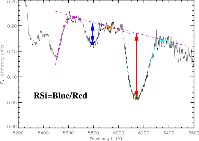
$\Re_{Si}$ is named for the characteristic Si ii trough found at $\approx 6100$Å and usually associated with the absorption trough of the Si ii$\lambda 6355$ Si ii line P-Cygni feature.

Fig. 1, illustrates the definition of $\Re_{Si}$, using the observed spectrum of SN 1992A 3 days after maximum. The dashed lines are the polynomial fits used to determine the maxima found in the wavelength zones defined in Table 1. The two depths are indicated by arrows.

The Si ii$\lambda 6355$ minimum band is centered on the Si ii$\lambda 6355$ line blueshifted approximately $10,000$ $\textrm{km}\leavevmode\nobreak\ \textrm{s}^{-1}$(Due to homologous expansion, it is customary to use velocities interchangeably with wavelength shifts when analyzing supernovæspectra.). The value of 10,000 $\textrm{km}\leavevmode\nobreak\ \textrm{s}^{-1}$corresponds to the average velocity at which the Si ii line is observed to form. The $\approx 200$Å  wide wavelength zone where we search for the second minimum is noted as “variable” because it is centered on the Si ii$\lambda 5972$ line blueshifted by nearly the same actual velocity as the Si ii$\lambda 6355$ minima. This to ensure that the right trough is found, which is assumed to be at least partly created by the Si ii$\lambda 5972$ Si ii line, thus it should form in the same physical region.

$\Re_{Si}$ is defined as the ratio of the vertical distances between each minima and the reference lines drawn between two consecutive maxima $d_{\textrm{blue}}$ and $d_{\textrm{red}}$, as shown in Fig. 1,

$$\textrm{$\Re_{Si}$}=\frac{d_{\textrm{blue}}}{d_{\textrm{red}}}.$$ (1)

This definition differs slightly from the one of Nugent et al. (1995), where tangents to the spectrum were manually selected instead of the reference lines between two consecutive maxima. These two methods mainly differ when the zones searched for maxima only display inflection points, but our method was easier to automate.

Finally, because it is defined as the distance between points of the spectrum and references linearly coupling points of the spectrum, $\Re_{Si}$is independent of the absolute flux calibration. Moreover, as it is calculated within a wavelength region only $\approx 1000$Å  wide, it will be relatively insensitive to both the relative flux calibration and reddening.

2.2 Definition of $\Re_{Ca}$

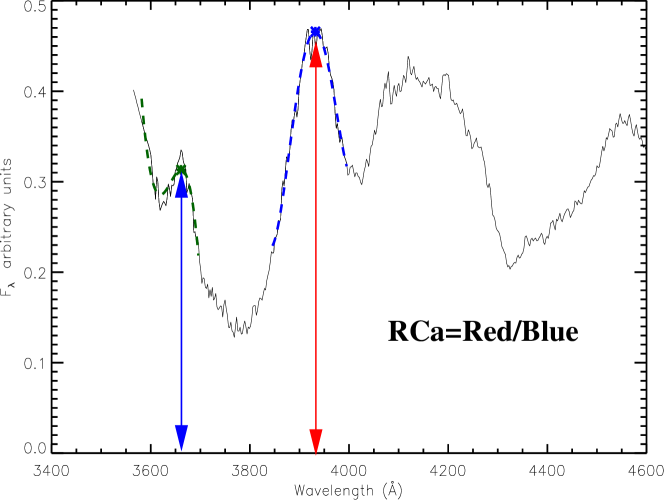
Following Nugent et al. (1995), we defined two zones in the $3000$Å–$4000$Å region of the spectrum, centered on the Ca ii $3650$Å and $3933$Å lines, as shown in the right hand side of Fig. 2. $\Re_{Ca}$ is defined as the ratio of the $\approx 3933$Å maximum, max$(F(3933))$, to the one at $\approx 3650$Å, max$(F(3650))$.

$$\textrm{$\Re_{Ca}$}=\frac{\mathrm{max}(F(3933))}{\mathrm{max}(F(3650))}$$ (2)

The width of the zones searched for these maxima are displayed in Table 2.

Table 2: $\Re_{Ca}$ Maximum Zones

Central Wavelength (Å)	Zone half-width (Å)
3650	48
3933	65

The maxima are almost never found at the exact wavelength of the Ca ii lines. This is expected since even if we had pure Ca ii, effects other than resonant-scattering could move the feature’s maximum wavelength. Moreover, these features are line blends, and not pure Ca ii lines.

The study of these wavelength zones with PHOENIX showed that the dominant elements of these blends had lines displaying the same qualitative evolution as $\Re_{Ca}$ with luminosity. This leads us to propose that the maxima ratio correlation with luminosity is only a corollary of the existence of a correlation between the blends. Hence, we defined an integral ratio we named $\Re_{CaS}$ (the S stands for surface) as

$$\textrm{$\Re_{CaS}$}=\frac{\int^{4012}_{3887}F_{\lambda}d\lambda}{\int^{3716}_{3620}F_{\lambda}d\lambda}$$ (3)

The wavelength regions were empirically chosen in order to group all the contributions with the same evolution with luminosity than $\Re_{Ca}$. We chose the wavelength limits in Eq. 3 in order to produce a spectral index that is well correlated to luminosity and robust to wavelength errors.

Both the $\Re_{Ca}$ and $\Re_{CaS}$ ratios, like $\Re_{Si}$, are independent of the absolute flux calibration, and not too sensitive to the relative calibration quality or reddening.

2.3 Dealing with Noise:

The main merit of $\Re_{CaS}$ over $\Re_{Ca}$ is the increased signal to noise ratio. On the other hand, $\Re_{Ca}$ and $\Re_{Si}$ will be highly sensitive to noise since they rely on maxima and minima detections. In order to reduce this effect, we fit each wavelength zone considered with a $4^{\textrm{th}}$ degree polynomial and search for their local maximum or minimum.

Because we want $\Re_{Si}$ and $\Re_{Ca}$ calculation algorithms to be automatic and robust, we need to search wavelength regions wide enough to be sure to find the right maxima and minima. But in these large zones the spectral feature shapes are more complex than that of a second degree polynomial. On the other hand, noise may generate oscillations which will be followed by a polynomial of too high a degree. We chose $6^{\textrm{th}}$ degree polynomials as they empirically proved to be a good compromise between these two effects.

3 Correlation of $\Re_{Si}$ & $\Re_{Ca}$  with Luminosity

Table 3: List of Observed supernovæ

SN	Epoch (day wrt max)	MB
SN 1998aq	-3, 0, 1, 2, 3, 4	-19.56
SN 1981B	0∗	-19.54
SN 1998bu	-4, -2, -1	-19.49
SN 1994D	2∗, 3∗, 4∗, 5∗, -3, -4, -5	-19.47
SN 1996X	-4, -2, 4, 0∗, 1∗	-19.43
SN 1989B	-1, -5	-19.42
SN 1992A	0, -1, -5, 3, 5	-19.32
SN 1986G	-1, -3, -5∗, 1, 3	-19.16 or -17.58

We applied these definitions to the public supernovæspectra we were able to gather, listed in Table 3. The absolute magnitudes of Reindl et al. (2005) are derived for a common arbitrary value of the Hubble Constant $H_{0}=60$$\mbox{km}\leavevmode\nobreak\ \mbox{s}^{-1}$ Mpc^-1. The values of the reddening and $\delta m_{15}$ were chosen to minimize deviations from the Hubble law for a set of 66 SNe Iain the Hubble flow. While other prescriptions for determining $M_{B}$ would give somewhat different results, with our small sample it is advantageous to use a single consistent prescription to determine $M_{B}$ rather than relying on a variety of methods to determine the distances to nearby SNe Ia. When present surveys that will construct large homogeneous samples of SNe Iain the Hubble flow are complete, it will be simple and necessary to redo our analysis. Nevertheless, we don’t expect to alter our qualitative conclusions. Reindl et al. (2005) were unable to determine a unique solution for the reddening to SN 1986G, and thus we have two $M_{B}$ values for SN 1986G which we carry through in our analysis. In the following, we will calculate results for both values of the absolute $B$ magnitude of SN 1986G, we will refer to the $M_{B}=-17.58$ case as “Case A”, and $-19.16$ as “Case B”. Since the analysis of Reindl et al. (2005) is the most recent and careful, we consider Case B to be the more likely value for $M_{B}$ and we will present plots of our results for Case B only, however since the reddening correction is uncertain and we are dealing with only a small number of supernovae, we will present our results for both cases in tabular form. For our calibration, we restrict ourselves to “Branch Normals” which we define to be SNe Iawith $-19.0<M_{B}<-19.8$, thus in Case A, SN 1986G is not included in the set of calibrators, whereas in Case B it is. As more spectra of SNe Ia with well-measured values of $M_{B}$ become available they are easily added to our analysis.

Even though $\Re_{Si}$ and $\Re_{Ca}$ were originally defined for SNe Iaspectra at maximum light, we used spectra ranging from $5$ days prior to maximum to $5$ days after maximum. We examined various epochs around maximum in order to determine whether or not the date of the spectra has a critical impact on the ratio’s correlation with luminosity. Moreover, since space programs like SNAP will only take one spectrum per supernova, we wanted to quantify the time window where spectra are usable for luminosity measures with line ratios. Note that JEDI proposes to take multiple spectra of each SN, at 5-day intervals in the observer’s frame.

On the other hand, because of time dilatation, the rise time for supernovæat $z\approx 1$ is twice as slow in the observer’s rest frame. Relaxing the time constraint to $\pm 5$ days around maximum was thus conservative.

3.1 $\Re_{Ca}$ & $\Re_{CaS}$ Correlation with Luminosity

Figure 3: $\Re_{Ca}$calculated using supernovælisted in Table 3 (Case B). The line is the result of the linear regression.

Figure 4: $\Re_{CaS}$calculated using supernovælisted in Table 3 (Case B). The line is the result of the linear regression.

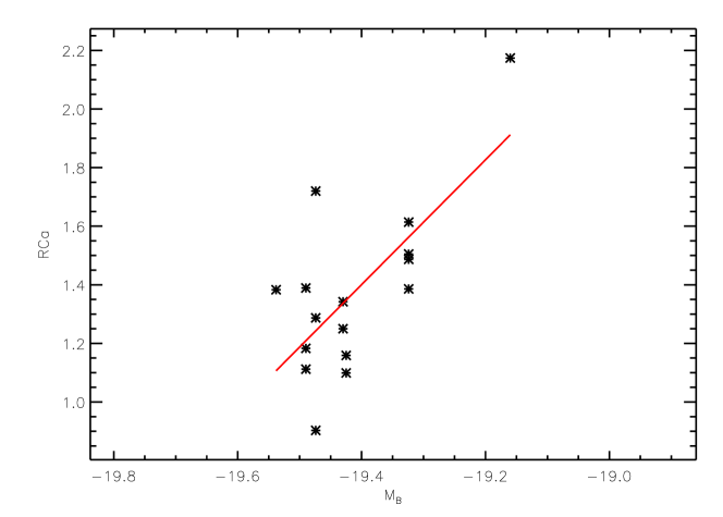
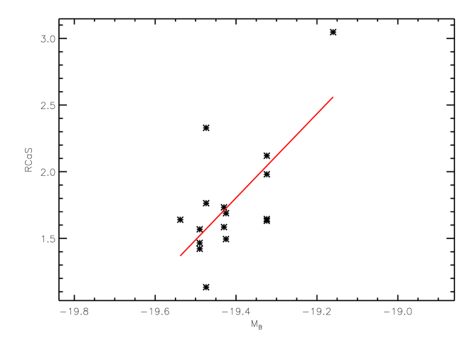
Some of the spectra listed in Table 3 lacked the wavelength coverage needed to calculate $\Re_{Ca}$ and $\Re_{CaS}$, those epochs are indicated with an asterisk. Neglecting these, the results for Case B are plotted in Figs. 3 and 4.

The $\Re_{Ca}$ values for maximum light spectra agree with Nugent et al. (1995) to within a few percent. In order to calibrate the luminosity relations, we computed the linear regression of $\Re_{Ca}$ and $\Re_{CaS}$ values with respect to blue magnitude. This linear regression should be valid in the restricted set of “Branch Normals”. 3-D deflagration models have difficulty reproducing the very low nickel mass of SN 1991bg-like supernovæand we illustrate below that synthetic spectra of W7 (Nomoto et al., 1984) indicate that there may be a departure of the spectral ratios from linearity for 1991T-like supernovæ. Thus, by restricting our calibrators to Branch Normals we might be using a more similar population. From the linear regression we obtain

$$\Re_{Ca} =a_{\textrm{$\Re_{Ca}$}}\leavevmode\nobreak\ M_{B}+b_{\textrm{$\Re_{Ca}$}}$$ (4)

$$\Re_{CaS} =a_{\textrm{$\Re_{CaS}$}}\leavevmode\nobreak\ M_{B}+b_{\textrm{$\Re_{CaS}$}}$$ (5)

We list the resulting parameters in Table 4. Since we have no information on the experimental errors, we set them arbitrarily equal to unity.

We also calculated the standard deviation $\sigma_{\textrm{$\Re_{Ca}$}}$ for $\Re_{Ca}$ and $\Re_{CaS}$, defined as the quadratic mean of the distance of each supernova from the linear regression, and have listed them in the same table. This definition of the error combines measurement errors, time dependence, and intrinsic dispersion.

Table 4: $\Re_{Ca}$ & $\Re_{CaS}$ luminosity measure precision

	$\sigma_{\textrm{$\Re_{Ca}$}}$	$a_{\textrm{$\Re_{Ca}$}}$	$\sigma_{M_{B}}$
$\Re_{Ca}$ (Case B)	0.20	2.1	0.10
$\Re_{CaS}$ (Case B)	0.31	3.1	0.10
$\Re_{Ca}$ (Case A)	0.19	1.2	0.16
$\Re_{CaS}$ (Case A)	0.39	1.4	0.28

Luminosity measure precision using $\Re_{Ca}$ or $\Re_{CaS}$:

With the linear regression calibration of $\Re_{Ca}$ and $\Re_{CaS}$ with respect to blue magnitude and the associated variance, we where able to estimate the luminosity precision measure using these ratios as follows:

$$\Re_{Ca} =a_{\textrm{$\Re_{Ca}$}}M_{B}+b_{\textrm{$\Re_{Ca}$}}$$

$$\sigma_{\textrm{$\Re_{Ca}$}} =a_{\textrm{$\Re_{Ca}$}}\sigma_{M_{B}}$$

$$\sigma_{M_{B}} =\frac{\sigma_{\textrm{$\Re_{Ca}$}}}{a_{\textrm{$\Re_{Ca}$}}}$$

$$\frac{\Delta L}{L} \approx\frac{\sigma_{\textrm{$\Re_{Ca}$}}}{a_{\textrm{$\Re_{Ca}$}}}$$

We display in Table 4 the present measurement accuracy on the blue magnitude as estimated for $\Re_{Ca}$ and $\Re_{CaS}$. We find in Case B that the accuracy of the method reaches the $0.1$ magnitude level.

3.1.1 $\Re_{Si}$ correlation with luminosity:

The correlation calibration

Figure 5: $\Re_{Si}$calculated using supernovæin Table 3 (Case B). The line is the result of our linear regression.

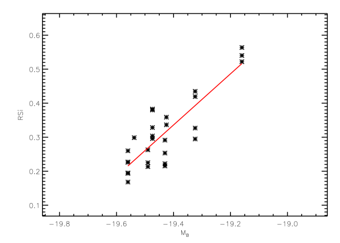
Fig. 5 shows the $\Re_{Si}$ values calculated with supernovæfrom Table 3, including spectra at all epochs. We excluded a negative $\Re_{Si}$ value from the $-5$ day SN 1994D spectrum, for which the blue trough associated with the Si ii$\lambda 5972$ feature does not exist. The $\Re_{Si}$ ratio is of course mathematically well defined even in this peculiar case, but since this point falls out of the general trend and increases the $\Re_{Si}$ slope, we removed it from the linear regression. This selection is compatible with observational constraints, as such spectra are easily identified when the signal to noise is large enough to measure $\Re_{Si}$.

The linear regression and the corresponding relative dispersion for this selection of supernovæis also shown in Fig. 5.

$$\textrm{$\Re_{Si}$}=a_{\textrm{$\Re_{Si}$}}M_{B}+b_{\textrm{$\Re_{Si}$}}$$ (6)

We also calculated the associated standard deviation and found it to be $\sigma_{\textrm{$\Re_{Si}$}}\approx 0.09$ (Case B) or $\sigma_{\textrm{$\Re_{Si}$}}\approx 0.06$ (Case A). This variance includes the measurement errors, time dispersion, as well as the intrinsic dispersion of the supernovæ.

Luminosity measure precision:

As in §3.1 we estimate the accuracy of the luminosity determination using $\Re_{Si}$ directly from the dispersion with respect to the linear regression. Table 5 summarizes the results.

Table 5: $\Re_{Si}$ luminosity measure precision

	$\sigma_{\textrm{$\Re_{Si}$}}$	$a_{\textrm{$\Re_{Si}$}}$	$\sigma_{M_{B}}$
$\Re_{Si}$ (Case B)	0.05	0.75	0.07
$\Re_{Si}$ (Case A)	0.06	0.59	0.10

4 $\Re_{SiS}$: A New Spectral Ratio

Figure 6: The definition of the method used for determining $\Re_{SiS}$. The arrows indicate the maxima used to compute $\Re_{SiS}$.

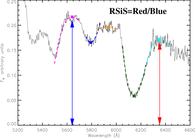
Due to the $\Re_{Si}$ correlation with luminosity, we have focused on the formation of features in the $\Re_{Si}$ zone. More will be said about the line formation in this spectral region in a forthcoming publication (S. Bongard et al., in preparation), but the clarification of the spectrum formation process led us to devise a new line ratio indicator which we call $\Re_{SiS}$.

$\Re_{SiS}$ is defined as the ratio of two maxima. The first maximum is the one used in the $\Re_{Si}$ calculation, located around Si ii$\lambda 6355$, and the second one is the bluer peak of due to sulfur (hence the name Si+S a mixture of silicon and sulfur) located in the $5600-5700$Å region as shown in Figure 6. The zones where we look for these maxima are listed in Table 6. As was the case for $\Re_{Si}$ and $\Re_{Ca}$, we used a 4${}^{\textrm{th}}$ order polynomial to fit the regions searched for the maxima, in order to increase robustness of the ratio with respect to Poisson noise.

Table 6: $\Re_{SiS}$ zones

	Lower Wavelength (Å)	Upper Wavelength (Å)
First maximum	6200	6450
Third maximum	5500	5700

We also define the integral ratio $\Re_{SiSS}$ as:

$$\mbox{$\Re_{SiSS}$}=\frac{\int_{5500}^{5700}F_{\lambda}d\lambda}{\int_{6450}^{6200}F_{\lambda}d\lambda}.$$ (7)

Once again, the simplicity of this integral ratio calculation and its insensitivity to noise makes it an interesting alternative to the line fitting method.

5 $\Re_{SiS}$ correlation with luminosity

Figure 7: $\Re_{SiS}$ (Case B) calculated using the supernovæof Table 3. The line is the result of our linear regression.

Figure 8: $\Re_{SiSS}$ (Case B) calculated using the supernovæof Table 3. The line is the result of our linear regression.

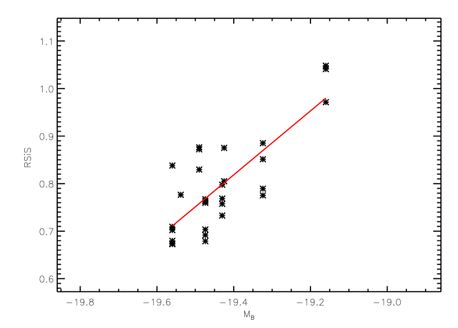
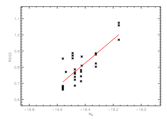
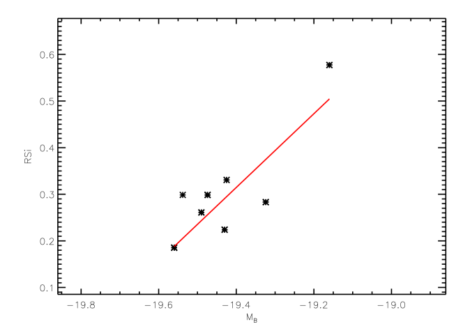
We plot the linear regression of $\Re_{SiS}$ correlation with luminosity in Fig. 7 We also plot in Fig. 8 the $\Re_{SiSS}$ correlation with luminosity. Table 7 summarizes the results for both quantities.

5.1 Luminosity measure precision

We summarize the different slopes and dispersion values for $\Re_{SiS}$ and $\Re_{SiSS}$ calculated with or without the time dispersion correction in Tables 7 and 10.

Table 7: $\Re_{SiS}$ luminosity measure precision

	$\sigma$	$a$	$\sigma_{M_{B}}$
$\Re_{SiS}$ (Case B)	0.06	0.67	0.09
$\Re_{SiSS}$ (Case B)	0.06	0.73	0.09
$\Re_{SiS}$  (Case A)	0.06	0.43	0.14
$\Re_{SiSS}$  (Case A)	0.07	0.53	0.11

With this spectral indicator family, even without time correction, we have augmented the blue magnitude accuracy by a factor of two compared to $\Re_{Ca}$. In Case A, $\Re_{Si}$ and $\Re_{SiS}$ have similar accuracies; however, in Case B $\Re_{SiS}$ is slightly better. Since $\Re_{SiS}$ and $\Re_{Si}$ cannot be considered as independent, we still have only two independent spectral indicators with $\Re_{Ca}$. But since one of them is as accurate as the light curve method, coupled with enough supernovæthey have the possibility to constrain evolutionary effects.

6 Time Evolution of Spectral Indices

Figure 9: $\Re_{Ca}$time evolution

Figure 10: $\Re_{CaS}$ time evolution

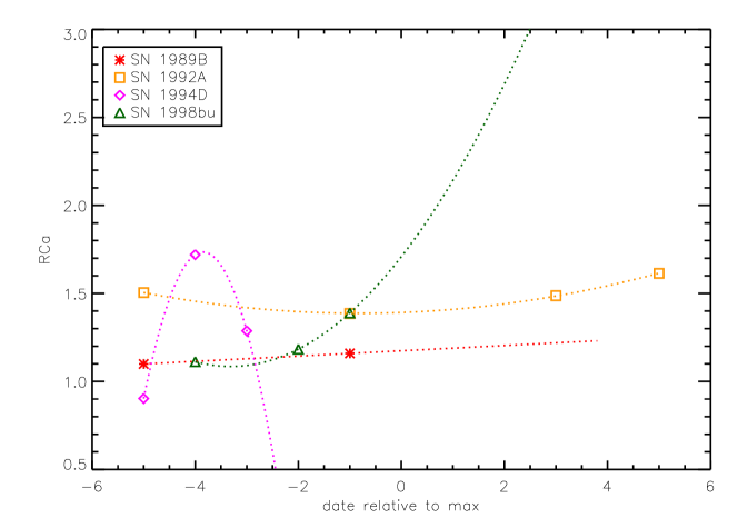
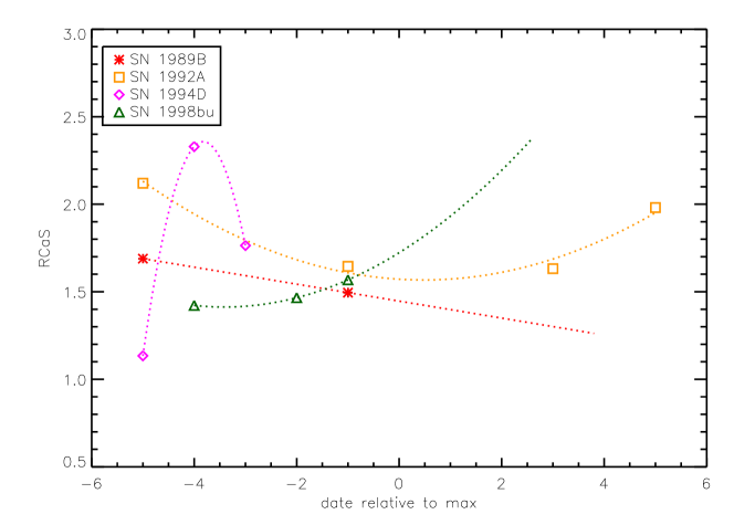
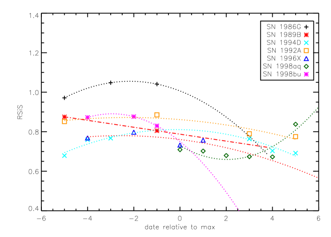
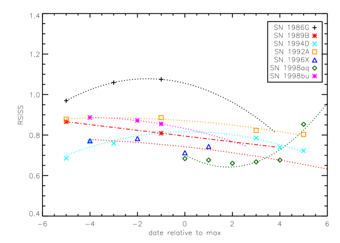
We plot in Fig. 9 and Fig. 10 the $\Re_{Ca}$ and $\Re_{CaS}$ time dependence for each supernova. Whenever enough data points were available, we interpolated the $t=0$ point using a $2^{\textrm{nd}}$ degree polynomial. For the cases with two points only, we used a straight line.

The supernova SN 1994D had enough points for a $2^{\textrm{nd}}$ order polynomial interpolation, but since all of them are for $t\leq-3$ days, and since the trend is different from the other supernovæ, we considered the $t=0$ point to be too much of an extrapolation to be used. Whether the SN 1994D dispersion in $\Re_{Ca}$ or $\Re_{CaS}$  is intrinsic or due to measurement uncertainties is still an open question.

Replacing each $\Re_{Ca}$ and $\Re_{CaS}$ by the corresponding $t=0$ calculated value, we recomputed the linear regression, and the associated standard deviation. These results are shown in Table 8.

Table 8: $\Re_{Ca}$ and $\Re_{CaS}$ interpolated linear regression

	$\sigma$	$a$	$\sigma_{M_{B}}$
$\Re_{Ca}$ (Case B)	0.26	0.93	0.27
$\Re_{CaS}$ (Case B)	0.35	1.19	0.30
$\Re_{Ca}$ (Case A)	0.23	0.48	0.48
$\Re_{CaS}$ (Case A)	0.24	0.75	0.31

More spectra are needed in order to show if there is a correlation in the evolution $\Re_{Ca}$ or $\Re_{CaS}$ with epoch, but it is apparent that there is no uniform trend with time, and the attempted correction to maximum light has increased the dispersion from Table 4 to Table 8. Therefore, it is conservative to treat the time dependence of $\Re_{Ca}$ and $\Re_{CaS}$ as an uncontrolled dispersion.

Fig. 11 displays the $\Re_{Si}$ time dependence of the supernovæwe used. We calculated a quadratic regression for each supernova with three or more $\Re_{Si}$ values. We then replaced each $\Re_{Si}$ value by the corresponding value at $t=0$ obtained via either interpolation or extrapolation. The new linear regression calculated for $\Re_{Si}$ correlation with luminosity is also plotted in Fig. 11. We calculated the same correction for the less favored luminosity choice for SN 1986G (Case A).

Table 9: $\Re_{Si}$ interpolated luminosity measure precision

	$\sigma_{\textrm{$\Re_{Si}$}}$	$a_{\textrm{$\Re_{Si}$}}$	$\sigma_{M_{B}}$
$\Re_{Si}$ (Case B)	0.06	0.79	0.07
$\Re_{Si}$ (Case A)	0.04	0.35	0.12

For the favored SN 1986G luminosity case (Case B) the extrapolation to $t=0$ significantly improves the measurement, as seen in Table 9 and lowers the dispersion to $0.1$ blue magnitude so that the $\Re_{Si}$ ratio probes “Branch normal” SNe Ialuminosities with good accuracy.

Figure 11: $\Re_{Si}$ time evolution (top panel, Case B) and $\Re_{Si}$ correlation with values interpolated to $t=0$ (bottom panel).

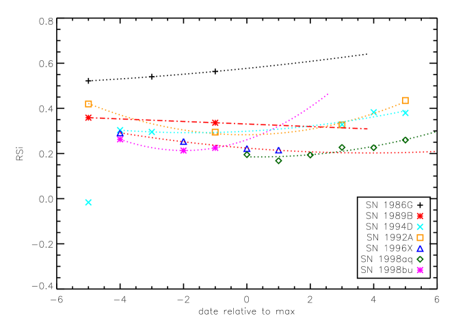
The standard deviation calculated with respect to this new regression, still removing the events with negative $\Re_{Si}$, is now $\sigma_{\textrm{$\Re_{Si}$}}\approx 0.07$ (Case B) or $\sigma_{\textrm{$\Re_{Si}$}}\approx 0.12$ (Case A). The top panel of Fig. 11 shows that there is no general time dependence trend for our supernovæsample.

In Fig. 12 and Fig. 13 we plot the time dependence of $\Re_{SiS}$ and $\Re_{SiSS}$ as well as the linear regression calculated on the values at $t=0$ interpolated or extrapolated with quadratic fits. The three supernovæwith sufficient data do not display a common time evolution, making doubtful the existence of an universal $\Re_{SiS}$ or $\Re_{SiSS}$ time correction.

Figure 12: $\Re_{SiS}$ time evolution (top panel), $\Re_{SiS}$  corrected for the time dependence (bottom panel).

Figure 13: $\Re_{SiSS}$ time evolution (top), $\Re_{SiSS}$  corrected for the time dependence (bottom).

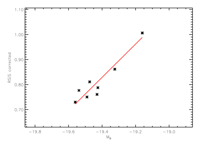
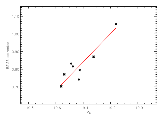
We again calculated the standard deviation, the results of the time correction are summarized in Tab. 10.

Table 10: $\Re_{SiS}$ and $\Re_{SiSS}$ linear regression with $t=0$ extrapolated values

	$\sigma$	$a$	$\sigma_{M_{B}}$
$\Re_{SiS}$ (Case B)	0.03	0.67	0.04
$\Re_{SiSS}$ (Case B)	0.04	0.80	0.05
$\Re_{SiS}$ (Case A)	0.02	0.49	0.05
$\Re_{SiSS}$ (Case A)	0.04	0.59	0.06

Correcting for the time evolution increases the $\Re_{SiS}$ and $\Re_{SiSS}$ efficiency both by increasing the slope and decreasing the dispersion, the only drawback is the need of at least three points to interpolate or extrapolate to $t=0$ with a quadratic fit. Since there is no common trend for the three supernovæthat were fit, this correction remains purely empirical.

7 Comparison with synthetic spectra

Figure 14: $\Re_{Ca}$ for Case B. Black: Observed supernovæ, Blue: day 20 W7 PHOENIX synthetic spectra, Pink: day 25 W7 PHOENIX synthetic spectra.

Figure 15: $\Re_{CaS}$ for Case B. Black: Observed supernovæ, Blue: day 20 W7 PHOENIX synthetic spectra, Pink: day 25 W7 PHOENIX synthetic spectra.

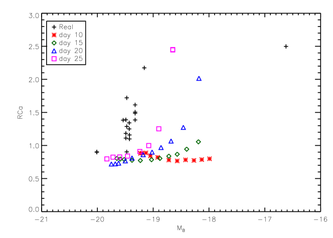
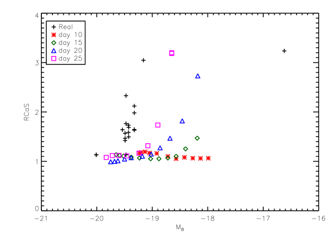
In order to ascertain whether the trends that we have found for the spectral indices can be reproduced by models, we have calculated a set of local thermodynamic equilibrium (LTE) models using the generalized stellar atmosphere code PHOENIX (Hauschildt & Baron, 1999, 2004) of the parameterized SN Ia deflagration model W7 where we varied the total luminosity bolometric luminosity in the observer’s frame. We calculated one set at 20 days after explosion (the fiducial time of maximum in $V$) and another at 25 days after explosion. We have assumed LTE for computational expedience. Studies by Baron et al. (1996) and Wheeler et al. (1998) have shown that LTE is a reasonable approximation in SNe Ia. The Si ii$\lambda 6355$ feature is not reproduced by W7, as shown by Baron et al. (2005), who used extremely detailed NLTE. Only the general trends of the synthetic spectra can then be expected to be matched by the real data. The use of PHOENIX with W7 models is described in detail in Lentz et al. (2001).

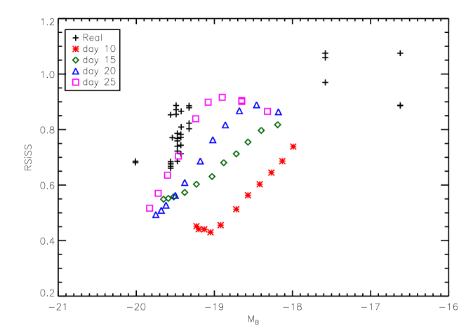
We display in Figs. 14–15 the comparison between $\Re_{Ca}$ and $\Re_{CaS}$ calculated on observed supernovæof Table 3 (all dates) and on PHOENIX spectra. These synthetic spectra cover a large range in $M_{B}$. Since the blue magnitude increases monotonically in the PHOENIX models with the bolometric magnitude, these figures indicate the existence of a spectroscopic sequence with the bolometric luminosity. The slope of the observed spectra is closer to that obtained from the models $25$ d after explosion. The increase in $\Re_{Ca}$and $\Re_{CaS}$ begins for lower blue magnitudes in the PHOENIX synthetic spectra than in the observed spectra.

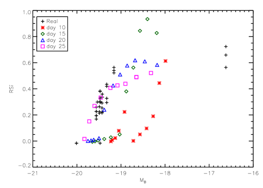
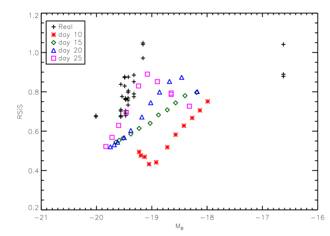
Figs. 16–18 display the same synthetic and observed spectra for $\Re_{Si}$, $\Re_{SiS}$, and $\Re_{SiSS}$. Again, the existence of the spectroscopic sequence is clear in both the observed and the synthetic spectra. Moreover, while the general trend is only qualitatively similar for $\Re_{Ca}$ and $\Re_{CaS}$, $\Re_{Si}$ and to a lesser extent $\Re_{SiS}$ and $\Re_{SiSS}$show that these ratio behave in the same way with respect to the blue magnitude evolution for synthetic as well as for real spectra.

Figure 16: $\Re_{Si}$ for $-19.16$ (top) and $-17.58$ (bottom) SN 1986G blue magnitude. Black: real supernovæ. Blue: day 20 W7 PHOENIX synthetic spectra. Pink: day 20 W7 PHOENIX synthetic spectra. For Day 10 there is a discontinuity in $\Re_{Si}$around $M_{B}=-18.9$, this is real and is caused by the change in the formation of the Si ii$\lambda 5972$ feature as discussed in Bongard et al.(in preparation). The very steep dependence of the various $\Re_{Si}$ ratios as of function of $M_{B}$ in the range $-19.5<M_{B}<-20$ is remarkably well reproduced by PHOENIX at day 25. The data points at low luminosity suggest a smaller slope. This justifies the limited luminosity range for the evaluation of the slopes in §§ 3–6

Figure 17: $\Re_{SiS}$ for $-19.16$ (top) and $-17.58$ (bottom) SN 1986G blue magnitude. Black: real supernovæ. Blue: day 20 W7 PHOENIX synthetic spectra. Pink: day 20 W7 PHOENIX synthetic spectra.

Figure 18: $\Re_{SiSS}$ for $-19.16$ (top) and $-17.58$ (bottom) SN 1986G blue magnitude. Black: real supernovæ. Blue: day 20 W7 PHOENIX synthetic spectra. Pink: day 20 W7 PHOENIX synthetic spectra.

8 Use of line ratios in the SNAP context

In order to estimate the luminosity measure accuracy of these spectral indicators in a cosmological context, we simulated SNAP exposures (SNAP Collaboration, 2005) at different redshifts. We used them to estimate the accuracy on the determination of the mean luminosity of “Branch normal” supernovæ, which is the value needed to devise the Hubble diagram and the determination of cosmological parameters.

8.1 SNAP simulator

8.1.1 The SNAP spectrometer

To simulate the SNAP spectrometer, we assumed $50\%$ optical and $70\%$ CCD efficiencies (Kim et al., 2004). We considered the mirror surface to be $\pi\leavevmode\nobreak\ m^{2}$ (i.e. a 2$m$ mirror diameter) and implemented the re-binning of the supernovæspectra to SNAP binning in the observer rest frame. The red and blue channel resolution of SNAP we used are summarized in Table 11 (A. Ealet, private communication; Ealet et al. [2003]).

Table 11: SNAP blue and red channel resolution

BLUE				RED
$\lambda$ (Å)	$\frac{\lambda}{\Delta\lambda}$	$\lambda$ (Å)	$\frac{\lambda}{\Delta\lambda}$	$\lambda$ (Å)	$\frac{\lambda}{\Delta\lambda}$	$\lambda$ (Å)	$\frac{\lambda}{\Delta\lambda}$
4000	295.	7500	95.
4500	235.	8000	90.
5000	185.	8500	85.
5500	155.	9000	80.
6000	130.	9500	78.
6500	115.	10000	75.
7000	105.
				10000.	78.	14000.	86.
				10500.	77.	14500.	90.
				11000.	77.	15000.	93.
				11500.	78.	15500.	97.
				12000.	79.	16000.	100.
				12500.	80.	16500.	105.
				13000.	82.	17000.	110.
				13500.	84.

The separation between the two spectrograph channels is not yet precisely defined, therefore we treated the spectra as if the red and the blue detector properties were the same. Since the edges of the spectral range are harder to calibrate, their actual location can impact the final results.

8.1.2 The simulated supernovæ

In order to simulate SNAP exposures, we calibrate each supernova to its absolute blue magnitude and then redshift it to the desired $z$.

$$N_{\gamma}(z)=N_{\gamma}(0)(1+z)\left(\frac{d_{0}}{d_{\mathrm{L}}}\right)^{2}$$ (8)

Eq. (8) shows how the number of photons per unit time and per unit area in the redshifted $B$ band in the supernova rest frame at redshift $z$, $N_{\gamma}(z)=\int_{B(z)}\frac{dN_{\gamma}(z)}{d\lambda}d\lambda$, is related to $N_{\gamma}(0)=\int_{B(0)}\frac{dN_{\gamma}(0)}{d\lambda}d\lambda$, the number of photons per unit of time and of surface in the B band at rest in the supernova rest frame for a supernova at 10 pc.

The flux dilution factor for a supernova at $z$ is $\frac{d_{0}^{2}}{d_{\mathrm{L}}^{2}}$ where $d_{0}=10$ pc, but the reddening factor $1+z$ included in $d_{\mathrm{L}}$ gets cancelled when photons are counted in redshifted spectral bands. We also introduced electronic and statistical noise using the values given in Table 12.

Table 12: Noise per pixel per 2000 s.

readout noise/pixel	$\sqrt{2}\cdot 5e$
slow drift contribution	$7\cdot 1.2e$
Leakage current fluct. for 2000s	$6e$
Total electronic noise per pixel:	$10e$
Presence of a cosmic ray ($20\%$ of cases)	$12e$
Total Electronic noise per $\Delta\lambda$ (3 spatial pixels)	$17e$

The electronic noise for each $2000s$ exposure was calculated using

$$n_{electronic}^{2}=17^{2}\cdot\frac{t}{2\times 10^{3}}$$ (9)

and assumed to be a Gaussian with zero mean. The Poisson noise of the signal was also included for each of the $2000$ s exposures needed to complete the total exposure time.

Table 13: SNAP simulator $N_{\gamma}\leavevmode\nobreak\ s^{-1}$ in Bessel B

$z$	Blue filter ($N_{\gamma}\leavevmode\nobreak\ s^{-1}\leavevmode\nobreak\ cm^{2}$)	Exposure Time
$1.0$	$4.32$	$5980s$
$1.5$	$1.75$	$22700s$
$1.7$	$1.3$	$36000s$

In Table 13 we display the number of photons per second expected in the B Bessel filter for a SN Iaof absolute blue magnitude $M_{B}=-19.42$, not accounting for the CCD and optical transmission. The exposure time we use have been assumed to follow a $(1+z)^{6}$ power law for $1<z<1.7$ and an exposure time of $10$ hours for $z=1.7$, chosen in order to maintain a constant signal to noise as $z$ increases (A. Ealet, private communication).

8.2 Results at $z=1.5$

Table 14: Supernovæsimulated in the SNAP context.

Supernova	Date (wrt maximum)	$M_{\textrm{B}}$
SN 1991T	$0$	$-20.01$
SN 1998aq	$0,1,2$	$-19.56$
SN 1981B	$0$	$-19.54$
SN 1998bu	$-2,-1$	$-19.49$
SN 1994D	$-3$	$-19.47$
SN 1996X	$-2,0,1$	$-19.43$
SN 1989B	$-1$	$-19.42$
SN 1992A	$-1$	$-19.32$
SN 1986G	$-1$	$-17.58$ or $-19.16$
SN 1991bg	$0$	$-16.62$

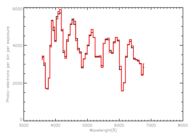
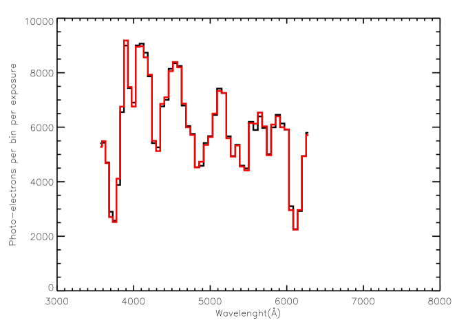
We display in Fig. 19 the number of photons per bin simulated obtained for the standard supernova SN 1992A at $z=1.5$ and $z=1.7$, respectively. This quantity differs from the usual flux per Å, which explains the flatter shape of the spectrum as there is a difference of $1/\lambda$ between them. For $z=1.7$, the wavelength coverage will be too small to allow the calculation of $\Re_{Si}$ and $\Re_{SiS}$, although it would be accessible to JEDI (the proposed spectroscopic wavelength coverage for JEDI is 0.8–2 $\mu$m).

We simulated 100 exposures for every supernova listed in Table 14 and calculated the spectral indicators previously defined for each of them and found the mean and standard deviation (see Tables 15, 16, 18, and 19). From this we calculate $\sigma_{M_{B}}$ assuming that the slope of the linear regression is known perfectly. In order to concentrate on the accuracy of the spectroscopic indicators in SNAP, and since at redshifts of $z\approx 1$ time dilatation doubles the evolution time of the light curve, we assumed that the spectra will be taken almost at maximum light. We thus included in our sample only the supernova spectra that were the close to the light curve maximum.

Figure 19: SNAP SN 1992A $z=1.5$ simulated exposure (top), and $z=1.7$ (bottom). Black curves are only the supernova, red curves include Poisson and electronic noise.

8.2.1 $\Re_{Si}$

We list in Table 15 the luminosities measured for the simulated supernovæwithout any selection cut on the simulated $\Re_{Si}$ values for Case A. The RMS dispersion due to the noise is displayed as well as the mean $\Re_{Si}$ used to calculate the blue magnitude. In this first table we used the linear regression calculated with $\Re_{Si}$ values extrapolated to $t=0$ when possible. Table 16 lists the same values but for the linear regressions corresponding to Case B. The large discrepancies observed for SN 1991T and SN 1991bg between the inferred (using $\Re_{Si}$) luminosity and the actual value suggests that the linear regression is invalid at low and high magnitudes, we discuss this further below; however, no firm conclusion can be drawn from the single cases in our current sample.

In order to estimate the mean accuracy for JDEM we add the values of $\delta M_{B}$ listed in the last column of the table in quadrature and divide by $N-2$. We lose two degrees of freedom by finding the mean and the slope with the same sample of supernovæin Tables 15–16 (and then we assume that the slope used is known perfectly); these values are listed in Table 24. Red, dim SN 1991bg-like SNe Ia will be strongly selected against due to Malmquist bias in deep cosmological surveys, therefore we shall never consider them in our analyses (in Case A we include SN 1986G in the 91bg-like class). Similarly SN 1991T-likes would also not be used for precision cosmology, but we quote results both including and excluding 91T-likes. In Case B where blue magnitude of SN 1986G is $M_{B}=-19.16$ as is favored by Reindl et al. (2005). the mean accuracy on the blue magnitude becomes $\approx 0.17(0.66)$ blue magnitude excluding (including) 91T-likes.

Table 15: $\Re_{Si}$ (Case A)

SN name	mean	$\sigma_{\textrm{$\Re_{Si}$}}$	Inferred $M_{B}$	$\sigma_{M_{B}}$	$\delta M_{B}$
91T	1.16	0.81	-16.84	2.34	-3.17
98aq	0.18	0.08	-19.66	0.23	0.10
81B	0.33	0.09	-19.24	0.26	-0.3
98bu	0.17	0.05	-19.70	0.16	0.21
94D	0.29	0.09	-19.35	0.27	-0.12
96X	0.27	0.09	-19.42	0.27	-0.01
89B	0.36	0.09	-19.14	0.33	-0.27
92A	0.26	0.11	-19.44	0.36	0.12
86G	0.32	0.16	-19.26	0.47	1.68
91bg	0.56	0.37	-18.58	1.09	1.96

Table 16: $\Re_{Si}$ (Case B)

SN name	mean	$\sigma_{\textrm{$\Re_{Si}$}}$	Inferred $M_{B}$	$\sigma_{M_{B}}$	$\delta M_{B}$
91T	1.16	0.81	-18.33	1.02	-1.68
98aq	0.18	0.08	-19.56	0.10	0.00
81B	0.33	0.09	-19.37	0.12	-0.16
98bu	0.17	0.05	-19.58	0.07	0.09
94D	0.29	0.09	-19.43	0.12	-0.04
96X	0.27	0.09	-19.46	0.12	0.02
89B	0.36	0.09	-19.34	0.15	-0.08
92A	0.26	0.11	-19.47	0.16	0.14
86G	0.32	0.16	-19.39	0.21	0.22
91bg	0.56	0.37	-19.08	0.48	2.47

Table 24 summarizes the total error expected in SNAP. We have calculated the total error by adding the “intrinsic $\sigma_{M_{B}}$” (obtained from the linear regression fit) in quadrature with the $\sigma_{M_{B}}$ estimated above due to noise from our simulations. We note that both error estimates include errors due to the same systematics and thus our estimate of the total error using Method 1 is quite conservative

We also note that our estimate of “the intrinsic $\sigma_{M_{B}}$” is strongly dependent on the slope of the linear regression and thus our restriction to Branch normals in obtaining the slope is optimistic. Nevertheless, the results of the synthetic spectral calculations bolster our view that the linearity is more pronounced in the Branch normal region. For $\Re_{Si}$, using the $t=0$ extrapolated linear regression instead of the one without correction increases the slope enough to give a significant effect in the less favored Case A, by $\approx 0.1$ blue magnitude. Thus, to take full advantage of this luminosity measure, we need spectra as close to to maximum light as possible, which will be feasible at $z=1.5$ since the elapsed time between $-1$ and $+1$ days around maximum is $2.5\times 2=5$ days and since SNAP will try to obtain spectra near peak to maximize signal to noise, the proposed JEDI mission will easily fulfill this goal since they will obtain multiple spectra every $\approx 7$ days.

Table 17: Number of supernovæin redshift bins for SNAP.

z	0.6	0.7	0.8	0.9	1.0	1.1	1.2	1.3	1.4	1.5	1.6	1.7
# of SN	150	171	183	179	170	155	142	130	119	107	94	80

As shown in Table 17, SNAP is expected to find $\approx 107$ SNe Iaat $z=1.5$. The accuracy expected on the luminosity measure with $\Re_{Si}$ would then be statistically improved by a factor of $\sqrt{107}\approx 10$ (although as discussed above this floor will truly be determined by the systematic error). The mean SNe Iablue magnitude at $z=1.5$ that is the quantity of cosmological interest, will be determined with an accuracy of $\approx(0.2)/10\approx 0.02$blue magnitude in Case A, excluding 91T-likes. Clearly in Case A if 91T-likes are included the method is not useful. It seems likely that 91T-likes will be identifiable by JDEM, so the smaller error is more reasonable. In Case B where its blue magnitude is $-19.16$, the mean accuracy would be $\approx(0.01-0.07)$, depending on whether 91T-likes are included. Thus $\Re_{Si}$ appears to be a good candidate for a supplementary tool to determine the equation of state of the universe using supernovæ.

8.2.2 $\Re_{SiS}$

In Tables 18, and 19 we list the results of our simulations for both Cases A and B. Table 24 shows that $\Re_{SiS}$ is clearly a superior luminosity indicator in that the total error is nearly constant at $\mathrel{\hbox{\hbox to0.0pt{\hbox{\lower 4.0pt\hbox{$\sim$}}\hss}\hbox{$<$}}}0.2M_{B}$ for all cases. This makes this ratio appear to be an excellent secondary probe of SNe Iablue magnitudes and to independently test evolutionary effects.

In Case B, where 91T-likes are rejected, the preferred case, the mean blue magnitude accuracy becomes $\approx 0.10$ blue magnitude, including 91T-likes increases the dispersion to only $0.16$ which is similar to the $\approx 0.2$ blue magnitudes dispersion of the SNe Iaafter stretch factor correction. We see that $\Re_{SiS}$ is more robust than $\Re_{Si}$ as the total error remains below $0.20$ blue magnitudes for any of our assumptions.

We found that $\Re_{SiSS}$ did not improve the results. This is due to the large wavelength binning in the SNAP design that already effectively transforms $\Re_{SiS}$ into an “integral” ratio compared to the $10$Å binning we previously used, as can be seen from the low dispersion due to Poisson noise($>5\%$). Thus $\Re_{SiSS}$ results are almost identical to those of $\Re_{SiSS}$, sometimes even a bit worse because the larger SNAP binning can include more of the Fe ii$\approx 5600$Å peak into the integral, reducing its quality as a luminosity indicator.

With more supernovæadded to our analysis it may be possible to include both 1991bg-like events into our calibration for the spectral indices.

Table 18: $\Re_{SiS}$ Case A

SN name	mean	$\sigma_{\mathrm{\Re_{SiS}}}$	Inferred $M_{B}$	$\sigma_{M_{B}}$	$\delta M_{B}$
91T	0.66	0.03	-19.71	0.07	-0.30
98aq	0.69	0.03	-19.64	0.06	0.08
81B	0.78	0.04	-19.47	0.07	-0.07
98bu	0.86	0.05	-19.31	0.11	-0.18
94D	0.77	0.04	-19.48	0.07	0.01
96X	0.74	0.04	-19.54	0.08	0.11
89B	0.83	0.06	-19.37	0.13	-0.05
92A	0.89	0.07	-19.24	0.15	-0.08
86G	1.06	0.07	-18.89	0.15	1.31
91bg	0.94	0.21	-19.15	0.43	2.52

Table 19: $\Re_{SiS}$ Case B

SN name	mean	$\sigma_{\textrm{$\Re_{SiS}$}}$	Inferred $M_{B}$	$\sigma_{M_{B}}$	$\delta M_{B}$
91T	0.66	0.03	-19.64	0.05	-0.36
98aq	0.69	0.03	-19.60	0.04	0.04
81B	0.78	0.04	-19.48	0.05	-0.06
98bu	0.86	0.05	-19.36	0.08	-0.13
94D	0.77	0.04	-19.49	0.05	0.01
96X	0.74	0.04	-19.53	0.05	0.10
89B	0.83	0.06	-19.40	0.10	-0.02
92A	0.89	0.07	-19.31	0.11	-0.01
86G	1.06	0.07	-19.04	0.11	-0.12
91bg	0.94	0.21	-19.23	0.32	2.61

8.2.3 $\Re_{Ca}$

Similar to $\Re_{SiSS}$, $\Re_{CaS}$  has a smaller dispersion due to noise, but a larger calibration error because of the coarse SNAP binning. We thus only display $\Re_{Ca}$ results in this section. $\Re_{Ca}$ calibration also suffers from the coarse sampling of SNAP spectrograph, as could be seen in the rightmost column of Tables 20–21. Since we found no trend with epoch, we have used the results for the slope without correction to $t=0$ (Table 4).

Table 20: $\Re_{Ca}$ Case A $z=1.5$

SN name	mean	$\sigma_{\textrm{$\Re_{Ca}$}}$	Inferred $M_{B}$	$\sigma_{M_{B}}$	$\delta M_{B}$
91T	0.88	0.03	-19.81	0.02	-0.20
81B	1.20	0.08	-19.53	0.07	-0.01
98bu	1.20	0.06	-19.53	0.05	0.04
94D	1.28	0.08	-19.46	0.07	-0.01
96X	1.42	0.08	-19.35	0.07	-0.08
89B	1.06	0.08	-19.65	0.07	0.23
92A	1.28	0.10	-19.47	0.08	0.15
91bg	2.43	1.71	-18.48	1.46	1.86

Table 21: $\Re_{Ca}$ Case B $z=1.5$

SN name	mean	$\sigma_{\textrm{$\Re_{Ca}$}}$	Inferred $M_{B}$	$\sigma_{M_{B}}$	$\delta M_{B}$
91T	0.88	0.03	-19.65	0.01	-0.36
81B	1.20	0.08	-19.49	0.04	-0.04
98bu	1.20	0.06	-19.49	0.03	0.00
94D	1.28	0.08	-19.46	0.04	-0.01
96X	1.42	0.08	-19.39	0.04	-0.04
89B	1.06	0.08	-19.56	0.04	0.14
92A	1.28	0.10	-19.46	0.05	0.14
91bg	2.43	1.71	-18.92	0.8	2.29

As can be seen in these tables that summarize the luminosity measure precision estimated for $\Re_{Ca}$, the systematic error dominates, the error due to the Poisson noise being always lower than $0.19$ blue magnitudes.

8.3 Evolution with $z$

SNAP wavelength coverage does not allow the use either $\Re_{Si}$, or $\Re_{SiS}$ for $z=1.7$. On the other hand $\Re_{Ca}$ will be measurable. JEDI would allow the measurement of $\Re_{Si}$ at $z=1.7$, but $\Re_{Ca}$  falls outside the range of its proposed IR spectrograph. Since the exposure time has been calculated so that the number of photons per bin will remain almost constant, the signal to noise will not be degraded too much. The dispersion due to noise (Tables 22–23 and Table 24) remains small compared to the intrinsic dispersion of the supernovæ.

Table 22: $\Re_{Ca}$ Case A $z=1.7$

SN name	mean	$\sigma_{\textrm{$\Re_{Ca}$}}$	Inferred $M_{B}$	$\sigma_{M_{B}}$	$\delta M_{B}$
91T	0.80	0.03	-19.87	0.02	-0.13
81B	1.32	0.07	-19.43	0.06	-0.11
98bu	1.26	0.14	-19.48	0.12	-0.00
94D	1.25	0.09	-19.49	0.07	0.02
96X	1.3	0.05	-19.45	0.04	0.02
89B	1.04	0.08	-19.67	0.07	0.25
92A	1.32	0.12	-19.42	0.1	0.1
91bg	2.39	1.41	-18.51	1.2	1.89

Table 23: $\Re_{Ca}$ Case B $z=1.7$

SN name	mean	$\sigma_{\textrm{$\Re_{Ca}$}}$	Inferred $M_{B}$	$\sigma_{M_{B}}$	$\delta M_{B}$
91T	0.80	0.03	-19.68	0.01	-0.33
81B	1.32	0.07	-19.43	0.03	-0.10
98bu	1.26	0.14	-19.47	0.06	-0.02
94D	1.25	0.09	-19.47	0.04	-0.00
96X	1.3	0.05	-19.45	0.02	0.02
89B	1.04	0.08	-19.57	0.04	0.15
92A	1.32	0.12	-19.43	0.06	0.11
91bg	2.39	1.41	-18.93	0.66	2.31

The $\Re_{Ca}$ blue magnitude accuracy remains dominated by the intrinsic dispersion of the supernovæcorresponding to $\sigma_{M_{B}}\approx 0.2$. This result can again be improved by using the $80$ supernovæexpected. The blue magnitude precision would then be $\Delta M_{B}\approx 0.02$, which is within the SNAP cosmological requirements.

Table 24: Summary of Spectral Indicator Precision for SNAP

Index	$\sigma_{M_{B}}$	$\sigma_{M_{B}}$	$\sigma_{M_{B}}$
	(intrinsic)	(noise)	(total)
$\Re_{Ca}$ ($z=1.5$, no 91T, Case A)	0.16	0.14	0.21
$\Re_{Ca}$ ($z=1.5$, with 91T, Case A)	0.16	0.16	0.23
$\Re_{Ca}$ ($z=1.5$, no 91T, Case B)	0.10	0.10	0.14
$\Re_{Ca}$ ($z=1.5$, with 91T, Case B)	0.10	0.19	0.21
$\Re_{Ca}$ ($z=1.7$, no 91T, Case A)	0.16	0.16	0.23
$\Re_{Ca}$ ($z=1.7$, with 91T, Case A)	0.16	0.15	0.22
$\Re_{Ca}$ ($z=1.7$, no 91T, Case B)	0.10	0.11	0.15
$\Re_{Ca}$ ($z=1.7$, with 91T, Case B)	0.10	0.18	0.20
$\Re_{Si}$ (no 91T, Case A)	0.12	0.24	0.27
$\Re_{Si}$ (with 91T, Case A)	0.12	1.31	1.32
$\Re_{Si}$ (no 91T, Case B)	0.10	0.14	0.17
$\Re_{Si}$ (with 91T, Case B)	0.10	0.65	0.66
$\Re_{SiS}$ (no 91T, Case A)	0.05	0.11	0.12
$\Re_{SiS}$ (with 91T, Case A)	0.05	0.16	0.17
$\Re_{SiS}$ (no 91T, Case B)	0.04	0.09	0.10
$\Re_{SiS}$ (with 91T, Case B)	0.04	0.16	0.16

9 Conclusions

We have presented a way to automatically measure the value of the spectral indices $\Re_{Ca}$ and $\Re_{Si}$, which should be robust. We have defined three new spectral indices $\Re_{CaS}$, $\Re_{SiS}$, and $\Re_{SiSS}$, which are less sensitive to noise in the spectrum. We have shown that for the limited set of Branch Normal supernovae where public spectra are available near maximum light that there is a good correlation between the spectral indices and the luminosity at peak. Within the caveat of small size of our sample we found that there is not a general trend in the spectral indices with epoch as long as the epoch is close to maximum light. We have used synthetic spectral models to show qualitatively that there does appear to be a deviation from linearity in the spectral indices, particularly among the dim, fast-declining supernovæ, such as SN 1991bg. This result is in agreement with that of Phillips et al. (1999) who also found that there is a deviation from linearity in peak magnitude with $\delta m_{15}$ as $\delta m_{15}$ increases (see their Figure 8). It is also in agreement with some theoretical hydrodynamical results which suggest it may be difficult to produce a SN Ia with such low nickel mass via a deflagration (W. Hillebrandt, private communication), although Höflich et al. (2002) are able to vary the nickel mass by varying the density of the deflagration to detonation transition. It has been suggested that there is both a variation in SNe Ialuminosity with galaxy type (Branch et al., 1996; Hamuy et al., 2001) and that there are two populations of SNe Iaprogenitors (Scannapieco & Bildsten, 2005; Mannucci et al., 2005) which could be related to the deviation in the linearity of the spectral indices.

Restricting ourselves to the sample of Branch Normal supernovæwe find that the proposed JDEM mission SNAP could in fact use $\Re_{SiS}$ as a complementary luminosity indicator. While the results may appear somewhat circular in that we have restricted our calibrators to have a small dispersion and then shown that the correlation based on that result also recovers the small dispersion, the ability to use a separate observable from light-curve shape will provide for a complementary measurement of the luminosity distance as a function of redshift in the proposed JDEM wide-field high-redshift spaced based surveys such as SNAP and JEDI. The lightcurve based method of template fitting will have a certain set of systematics that depends on exactly how “like versus like” is chosen, whereas the spectral index method will have a different set of systematics. In addition, the spectral index methods are very weakly sensitive to both the effects of dust and of the flux calibration of the spectrum, since they are defined in a very narrow wavelength range.

Our simulations show that the single spectrum obtained by SNAP for type identification will have sufficient signal to noise to measure the spectral indices to the required precision. JEDI, which will obtain multiple spectra for each supernova, would be even better suited to using $\Re_{SiS}$ since they would have a larger sample of spectra very close to maximum light.

As more spectra from nearby supernovæwith known peak luminosities become available we should be able to refine our calibration, and thus improve its accuracy for JDEM and other supernovæsurveys. We note that our actual numerical results rely on both a very small sample and also on the value of the absolute magnitudes assigned by Reindl et al. (2005), although since we quote results with both Case A and B the sensitivity to the assigned absolute magnitudes can be gauged somewhat. All available distance estimates (and hence absolute magnitudes) to our sample will contain errors, and we have chosen to use the results of Reindl et al. (2005) because they are derived in a specific somewhat homogeneous manner. Thus, we regard this work as a “proof of concept” and the specific numerical values as our best current estimate. Clearly when 300 Hubble-flow supernovae are available from current ground-based surveys (i.e. in the next 3-5 years), this analysis should be recomputed. Once accurate values are in hand, comparing absolute magnitude (determined from light-curve shape) and $\Re_{SiS}$ determined at high redshift may provide a useful measure of the evolutionary effects in the high-redshift sample. We discuss this further in a forthcoming publication where we study the formation of the Si ii$\lambda 5972$ line.

References

- Aldering et al. (2004) Aldering, G. et al. 2004, PASP, submitted, astro-ph/0405232
- Baron et al. (2005) Baron, E., Bongard, S., Branch, D., & Hauschildt, P. 2005, ApJ, submitted
- Baron et al. (1996) Baron, E., Hauschildt, P. H., Nugent, P., & Branch, D. 1996, MNRAS, 283, 297
- Branch et al. (1993) Branch, D., Fisher, A., & Nugent, P. 1993, AJ, 106, 2383
- Branch et al. (1996) Branch, D., Romanishin, W., & Baron, E. 1996, ApJ, 465, 73
- Crotts et al. (2005) Crotts, A., Garnavich, P., Priedhorsky, W., Habib, S., Heitmann, K., Wang, Y., Baron, E., Branch, D., Moseley, H., Kutyrev, A., Blake, C., Cheng, E., Dell’Antonio, I., Mackenty, J., Squires, G., Tegmark, M., Wheeler, C., & Wright, N. 2005, Joint Efficient Dark-energy Investigation (JEDI): a Candidate Implementation of the NASA-DOE Joint Dark Energy Mission (JDEM), Tech. rep., White paper to the Dark Energy Task Force
- Ealet et al. (2003) Ealet, A. et al. 2003, in IR Space Telescopes and Instruments, Proceedings of the SPIE, ed. J. Mather, Vol. 4850, 1169–1178
- Garnavich et al. (1998) Garnavich, P. M. et al. 1998, ApJ, 493, L53
- Garnavich et al. (2004) —. 2004, ApJ, 613, 1120
- Goldhaber et al. (2001) Goldhaber, G. et al. 2001, ApJ, 558, 359
- Hamuy et al. (2001) Hamuy, M., Trager, S., Pinto, P., Phillips, M., Schommer, R., Ivanov, V., & Suntzeff, N. 2001, AJ, 120, 1479
- Hauschildt & Baron (1999) Hauschildt, P. H. & Baron, E. 1999, J. Comp. Applied Math., 109, 41
- Hauschildt & Baron (2004) —. 2004, Mitteilungen der Mathematischen Gesellschaft in Hamburg, 24, 1
- Höflich et al. (2002) Höflich, P., Gerardy, C., Fesen, R., & Sakai, S. 2002, ApJ, 568, 791
- Kim et al. (2004) Kim, A. G., Linder, E. V., Miquel, R., & Mostek, N. 2004, MNRAS, 347, 909
- Kowal (1968) Kowal, C. T. 1968, AJ, 73, 1021
- Lentz et al. (2001) Lentz, E., Baron, E., Branch, D., & Hauschildt, P. H. 2001, ApJ, 557, 266
- Mannucci et al. (2005) Mannucci, F., Della Valle, M., & Panagia, N. 2005, MNRAS, in press, astro-ph/0510315
- Mazzali et al. (1997) Mazzali, P. A., Chugai, N., Turatto, M., Lucy, L. B., Danziger, I. J., Cappellaro, E., della Valle, M., & Benetti, S. 1997, MNRAS, 284, 151
- Nomoto et al. (1984) Nomoto, K., Thielemann, F.-K., & Yokoi, K. 1984, ApJ, 286, 644
- Nugent et al. (1995) Nugent, P., Phillips, M., Baron, E., Branch, D., & Hauschildt, P. 1995, ApJ, 455, L147
- Perlmutter et al. (1999) Perlmutter, S. et al. 1999, ApJ, 517, 565
- Phillips (1993) Phillips, M. M. 1993, ApJ, 413, L105
- Phillips et al. (1999) Phillips, M. M., Lira, P., Suntzeff, N. B., Schommer, R. A., Hamuy, M., & Maza, J. 1999, AJ, 118, 1766
- Reindl et al. (2005) Reindl, B., Tammann, G. A., Sandage, A., & Saha, A. 2005, ApJ, 624, 532
- Riess et al. (1998) Riess, A. et al. 1998, AJ, 116, 1009
- Riess et al. (1995) Riess, A. G., Press, W. H., & Kirshner, R. P. 1995, ApJ, 438, L17
- Scannapieco & Bildsten (2005) Scannapieco, E. & Bildsten, L. 2005, ApJ, 629, L85
- SNAP Collaboration (2005) SNAP Collaboration. 2005, Supernova Acceleration Probe: Studying Dark Energy with Type Ia Supernovae, Tech. rep., White paper to the Dark Energy Task Force
- Wheeler et al. (1998) Wheeler, J. C., Höflich, P., Harkness, R. P., & Spyromilio, J. 1998, ApJ, 496, 908
- Wilson (1939) Wilson, O. C. 1939, ApJ, 90, 634