Star-burst regions in the LMC

Aims. Filamentary structures of early type stars are found to be a common feature of the Magellanic Clouds formed at an age of about $0.9-2\times 10^{8}\,yr$. As we go to younger ages these large structures appear fragmented and sooner or later form young clusters and associations. In the optical domain we have detected 56 such large structures of young objects, known as stellar complexes in the LMC for which we give coordinates and dimensions. We also investigate star formation activity and evolution of these stellar complexes and define the term “starburst region”. Methods. IR properties of these regions have been investigated using IRAS data. A colour-magnitude diagram (CMD) and a two-colour diagram from IRAS data of these regions ware compared with observations of starburst galaxies and cross-matching with HII regions and SNRs was made . Radio emission maps at 8.6-GHz and the CO (1$\rightarrow$0) line were also cross correlated with the map of the stellar complexes. Results. It has been found that nearly 1/3 of the stellar complexes are extremely active resembling the IR behaviour of starburst galaxies and HII regions. These stellar complexes illustrating such properties are called here “starburst regions”. They host an increased number of HII regions and SNRs. The main starburst tracers are their IR luminosity ($F_{60}$ well above 5.4 Jy) and the 8.6-GHz radio emission. Finally the evolution of all stellar complexes is discussed based on the CO emission.

1 Introduction

Due to its proximity to our Galaxy and the SMC, the LMC offers two important advantages: i) the possibility to study its stellar content down to low stellar masses and ii) the possibility to follow the consequences of the close interaction, about $2-4\times 10^{8}\,yr$ ago (Gardiner & Noguchi gardiner (1996); Kunkel, Demers & Irwin kunkel (2000)), with the SMC. Stellar complexes are defined as large structures (clump like) in galaxies dominated by recently formed stellar component mixed with very young clusters, stellar associations and gas (Martin et al. martin (1976); van den Bergh van (1981); Elmegreen & Elmegreen elmegreen2 (1983); Feitzinger & Braunsfurth feitz (1984); Elmegreen & Elmegreen elmegreen3 (1987); Ivanov ivanov (1987); Larson et al. larson1 (1988); Efremovefremov1 (1989); Larson et al. larson2 (1992); Efremov & Chernin efremov3 (1994); Elmegreen et al. elmegreen4 (1994); Kontizas et al. kontizas1 (1994); Efremov efremov2 (1995); Battinelli, Efremov & Magnier battinelli (1996); Elmegreen & Efremov elmegreen1 (1996); Kontizas et al. kontizas2 (1996)). So far they have been detected as regions with young stellar component and enhanced stellar number density, compared to the surrounding region. In the LMC stellar complexes have been detected using UK Schmidt plates (Maragoudaki et al. maragoudaki1 (1998)). In the optical domain we have detected 56 large structures of young objects. These stellar complexes are associated with the already known nine Shapley constellations (Shapley shapley (1956)), which are referred to as large stellar structures of early type supergiants.

Helou (helou (1986)) found that the IRAS $log(F_{60}/F_{100})$ versus $log(F_{12}/F_{25})$ colour-colour diagram of “normal galaxies” shows a distribution that extends continuously from the cool ($\sim$20K) relatively constant “cirrus” emission from the neutral medium to the warmer ($\sim$40-50K) emission from the active, starburst end.

IRAS far-IR fluxes for 6 HII regions in the LMC have been studied by DeGioia-Eastwood (gioia (1992)). These regions are the sites of massive star formation, where the radiative heating source is young stars rather than the general interstellar radiation field. Such regions are expected to lie in stellar complexes and/or to be the stage just before the stellar complex is formed.

The highly structured diffuse X-ray emission of the LMC has been imaged in detail by ROSAT. The brightest regions are found east of LMC X-1 and in the 30 Doradus region. The latter is strikingly similar to the optical picture. There is a strong correlation between diffuse features in the X-ray image and ESO colour images of the LMC in visible light. Bright knots in the X-ray map correspond to HII emission in the optical (Westerlund west (1997)). The distribution of the SNRs in the LMC shows (i) a clumping of objects in the 30 Doradus region, (ii) several remnants within the Bar of the LMC and (iii) that the remainder of the remnants are found in super-associations. Most SNRs in the Bar are in regions where many young clusters are located, clusters as young as $\leq\,10\,Myr$ (Westerlund west (1997)).

The LMC has been well studied in the radio continuum, which is connected to the formation of new and massive stars. Fukui et al. (fukui1 (1999), fukui2 (2001)) found that the molecular clouds in the LMC have a good correlation with the youngest ($\la$10 Myr) stellar clusters, while there is little spatial correlation of these clouds with SNRs or with the older stellar clusters.

In this paper we describe how the stellar complexes were detected, using optical data and we give their location and dimensions. The total flux of each structure is presented. Their derived IR properties are compared to IR properties of galaxies in order to identify the distinction between ordinary stellar complexes and active star formation regions. Possible connection of the complexes determined here with known X-ray detected SNRs and candidates as well as HII regions is discussed. Finally, their correlation between high resolution radio data at 8.6-GHz and CO emission is examined, in order to determine the activity of the complexes and their evolution.

2 Optical data

The large-scale structures in nearby galaxies require extended field observational material in order to be treated homogeneously. Therefore we used direct photographic plates taken with the UK 1.2m Schmidt Telescope, in various wavebands: U, R and HeII ($\lambda=4686$ Å) down to a magnitude limit of $19-20\,mag$. These plates were digitised using the fast measuring machines APM and SuperCosmos. The derived data were produced as catalogues of detected stellar images. Star counts were performed on the above catalogues in order to derive isopleth contour maps of the LMC in the various wavebands and magnitude slices, to trace the differences between faint and brighter stellar populations. Star counts, in the optical wavelength range, of large areas in the LMC have revealed 56 groupings of young stars, known as stellar complexes (with dimensions from 150 $pc$ to $\sim$ 1500 $pc$). Their coordinates, dimensions and properties are given in Table 2, whereas their ages span from a few $\times 10^{8}\,yr$ to very young ($\sim 10^{6}\,yr$). The ages are derived from their stellar component, as described by Maragoudaki et al. (maragoudaki1 (1998)), which consist of early type stars (O, B, A), dust, young clusters and associations, very often in groups. The parental density fluctuations, which were fragmented into stellar complexes can be explained as a result of the close encounter of the SMC with the LMC that happened a few $\times 10^{8}\,yr$ ago (Gardiner & Noguchi gardiner (1996); Kunkel et al. kunkel (2000)).

3 IR data

IRAS all-sky survey Images taken at 12, 25, 60 and 100 $\mu$m have been obtained from SkyView (http://skyview.gsfc.nasa.gov/skyview.html) for the whole area of the LMC to study the IR properties of the stellar complexes detected in the optical domain. From the IRAS catalogues we calculated a total flux for each complex as the sum of the fluxes corresponding to the pixels, which cover the predetermined complex area. These total fluxes were corrected from the background. The background value was assumed as the average of four flux/pixel values at the four rather clear corners of each frame, for all IRAS wavelengths respectively. The background corrected total fluxes were averaged to a mean value (flux/pixel in MJy/sr) for all complexes so that they can be more easily compared with the literature.

Fig. 1 shows the IRAS colour-colour diagram of $log(F_{25}/F_{12})$ vs $log(F_{60}/F_{25})$ for the detected stellar complexes. The black-filled squares represent the integrated values for NGC1068, M82, M31 and LMC respectively, indicating the loci of different types of galaxies on this diagram. NGC1068 is a prototype AGN (Rowan-Robinson & Crawford rowan1 (1989)), M82 is a prototype starburst galaxy, while M31 is a typical disk galaxy (Rice, W., et al. rice (1988)). The LMC HII regions of DeGioia-Eastwood (gioia (1992)) are plotted with circles. We notice that many stellar complexes lie around the location of M82, a prototype starburst, and the HII regions revealing enhanced star formation activity.

Figure 1: IRAS colour-colour diagram for the detected stellar complexes. The black-filled squares mark the observed colours of the LMC (irregular galaxy) and three typical galaxies: M31 (disk), M82 (starburst) and NGC1068 (AGN). The circles mark LMC HII regions.

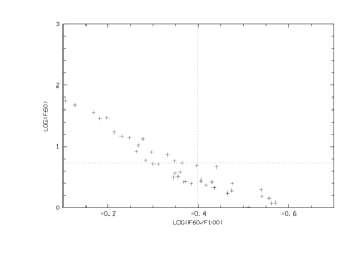
Figure 2: IRAS flux density in $logF_{60}$ versus IRAS colour $log(F_{60}/F_{100})$ for all the structures detected here. Two lines are plotted which represent $F_{60}=5.4\,Jy$ and $F_{60}/F_{100}=0.4$. The upper left area indicates the loci of very active star forming regions.

The IRAS flux densities in $logF_{60}$ versus the IRAS colour $log(F_{60}/F_{100})$ for all the large structures detected here are illustrated in Fig. 2. Lehnert & Heckman (lehnert (1996)) seeking to improve our understanding of the range of physical processes occurring within IR selected galaxies, found that the starburst galaxies are IR “warm” if $F_{60}/F_{100}\geq 0.4$ ($log(F_{60}/F_{100})\geq-0.39$) and IR “bright” if $F_{60}\geq 5.4$ Jy ($log(F_{60})\geq 0.73$). From Fig. 2 it is obvious that nearly 1/3 of the detected stellar complexes fulfil the criteria defined by Lehnert & Heckman (lehnert (1996)) for the starburst galaxies. The three upper points correspond to regions in 30 Doradus (complexes C17, A21, A24), where there is the highest concentration of SNRs. The 15 structures that have $log(F_{60}/F_{100})\geq-0.39$ and $log(F_{60})\geq 0.73$, resemble the behaviour of starburst galaxies, whereas the rest 41 do not show enhanced star formation activity.

4 Radio and CO data

We used the recently published 8.6-GHz map of Dickel et al. (dickel (2005)), with its angular resolution of 20″ and linear resolution $\sim$5 pc and the CO (1$\rightarrow$0) line that was fully mapped by Fukui et al. (fukui1 (1999)), with angular resolution of 2.6′ corresponding to a spatial resolution of $\sim$40 pc. In Fig. 3 we have superimposed the stellar aggregates, complexes and super-complexes (yellow lines) onto the radio 8.6-GHz (grey-scale) and CO (red contours) map. The time sequence evident in this figure is such that the molecular gas (CO) traces regions of ongoing and (near-) future star formation, the ionised gas (8.6-GHz) locates ongoing and somewhat evolved star formation ($10^{7}$ $\sim$ $10^{8}$ yr). We examined the correlation between 8.6-GHz radio emission, the CO emission and the location of the 56 stellar complexes (Table  2, columns 8 and 9).

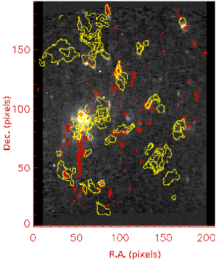
Figure 3: Maps of the LMC at 8.6 GHz (grey-scale) and in the CO(1$\rightarrow$0) line (red contours), with the stellar complexes superimposed with yellows lines.

We notice that the majority (13 out of 15) of the regions with $F_{60}>5.4Jy$, coincide well with the 8.6-GHz radio emission. The existence of CO emission in seven of them, reveals future star formation activity. The rest 2, that lack both 8.6-GHz and CO radiation, are actually found to have values of $F_{60}$ very close to $5.4Jy$. Considering the 41 regions with $F_{60}<5.4Jy$, the opposite behaviour is revealed. 36 out of 41 regions do not exhibit significant amount of 8.6-GHz radiation, while the remaining 5 that do exhibit 8.6-GHz radiation, are found to have $F_{60}$ very close to $5.4Jy$.

The CO emission is indicative of on-going and possible future star formation activity and there is no pattern revealed regarding the $F_{60}$ of the complexes. 16 out of the 56 complexes have significant CO emission, indicating possible future star formation activity and only 10 of them are correlated with 8.6-GHz emission as well.

5 Discussion & Conclusions

From optical observations, 56 stellar complexes are revealed in an area of $6\times 7\deg^{2}$ of the LMC. The IR properties are studied using the IRAS fluxes. The ratio of the flux densities $F_{60}/F_{100}$, the flux density $F_{60}$ as discussed above, the 8.6-GHz and CO radio emission, will be used in order to classify these complexes.

As mentioned in section 3, Lehnert & Heckman (lehnert (1996)) showed that starburst galaxies are IR “warm” and “bright”. In the same manner, we adopt the equivalent term “starburst regions” for complexes that are found to fulfil these criteria, namely $F_{60}/F_{100}\geq 0.4$ and $F_{60}\geq 5.4$ Jy. In addition, complexes that do not fulfil the previously stated criteria will be called “active complexes”.

A more detailed study of high resolution 8.6-GHz map (Fig. 3) revealed that all complexes with F₆₀ well above the 5.4 Jy limit are very well correlated with the 8.6-GHz radio emission. In contrast, complexes with F₆₀ well below the 5.4 Jy limit lack 8.6-GHz emission. However, 7 out of the 56 complexes (A5, A6, A7, C5, C7, C22 and A31) have F₆₀ close to the classification limit and deviate from the above behaviour. Complex C22, for example, is well correlated with 8.6-GHz emission; its F₆₀(5.07$\pm 0.20$ Jy) though is below the accepted limit. In contrast A31 has F₆₀=5.98$\pm 0.20$ Jy, which would classify it as a starburst region; however, there is no 8.6-GHz emission associated with it. Since the $F_{60}$ criterion is not trustworthy for these regions, we additionally use the 8.6-GHz emission to classify the complexes as “starburst candidates” or “active complexes candidates” depending on its existence. Hence, using the 8.6-GHz radiation as an additional tracer in tandem with the $F_{60}$, we can classify the stellar complexes into 13 starbursts, 5 starburst candidates, 2 active complexes candidates and 36 active complexes as seen in Table  1. The characterisation of each complex is given in Table  2, column 10.

Table 1: Complexes characterisation.

Complex Type	$F_{60}$	8.6	No. of
	(Jy)	(GHz)	Complexes
starburst	$F_{60}>$5.4	yes	13
starburst candidate	$F_{60}\la$5.4	yes	5
active complex candidate	$F_{60}\ga$5.4	no	2
active complex	$F_{60}<$5.4	no	36

Moreover, a discrimination concerning the evolution of all the complexes was attempted based on the CO data. More than half of the starburst and starburst candidate regions show enhanced CO emission indicating ongoing and future evolution, while the rest of them are thought to be more or less evolved. Regarding the active stellar complexes (and the two candidates), we found only 5 of them with significant amount of CO emission, giving additional indication of current star formation and revealing potential future starbursts. The lack of CO in the rest of them could indicate that these complexes have never been starbursts or that their starburst activity previously exhausted the molecular gas.

Figure 4: The HII regions (triangles) and SNRs (squares), plotted over the stellar complexes as defined here.

In Fig. 4 we plotted the known SNRs and HII regions based on the literature (Williams et al. williams (1999); Haberl & Pietsch haberl (1999); Filipovic et al. filip (1998) and Sasaki, Haberl & Pietsch sasaki (2000)) over the stellar complexes with triangles and squares respectively. The overplotted HII regions show an increased concentration in and around the very active star forming regions, as expected. Most of the defined starburst areas (and the candidates) are associated with SNRs. The detected complexes are also cross-matched with the catalogue of stellar associations (Gouliermis et al. gouliermis (2003)) and that of nebulae in the LMC (Davies, Elliot & Meaburn davies (1976)). The majority of the complexes are loci of stellar associations, whereas all of them are associated with a large number of nebulosities (Table  2).

Table 2: List of the LMC stellar complexes. Col. 1 indicates the adopted identification name. A denotes aggregate, C complex and SC super-complex. For a structure found inside a larger one, the name of the later is given in parenthesis. Col. 2, 3 and 4 give the RA, DEC of the “centre” of each stellar complex and its dimension. Col. 5,6, 7 show the number of SNRs and candidates, stellar associations and number of Nebulae and Henize objects found in each complex. Col. 8 and 9 indicate presence of 8.6-GHz and CO line emission respectively. Finally in Col. 10 the complexes are characterised. I indicates starbursts, II starburst candidates, III active complexes candidates and IV active complexes.

Stellar grouping	RA (1950)	DEC (1950)	Dimension	No.SNRs	Association ID	No.Nebulae	8.6	CO	Characterisation
	h m s	deg m s	(pc)				GHz	line
SC1	05:44:39	-67:15:18	1421.5	1	173,257	46	-	-	IV
C1 (SC1)	05:43:30	-67:17:29	355.3	0	173,257	57	-	-	IV
A1	05:52:53	-67:29:46	205	0	173,257	22	-	-	IV
A2	05:43:44	-67:19:37	191	1	173,257	31	-	-	IV
SC2	05:31:22	-66:54:42	1526.5	7		24	-	-	IV
C2 (SC2)	05:32:45	-67:05:11	749	1	173	41	-	-	IV
C3 (C2)	05:32:47	-66:58:22	572	1		32	-	-	IV
A3 (SC2)	05:29:45	-66:37:17	204	0		31	-	-	IV
A4 (C2)	05:30:53	-66:39:15	245	0		26	-	-	IV
A5 (SC2)	05:32:55	-67:32:29	164	1	173,257	41	-	-	III
A6	05:25:58	-66:12:18	299	1		20	$\surd$	$\surd$	II
A7	05:27:01	-67:27:42	299	1	173,257	10	$\surd$	-	II
C4	05:13:28	-67:20:57	314	0	173,257	16	-	-	IV
A8 (C4)	05:13:10	-67:22:34	246	0	173,257	16	-	-	IV
A9	05:10:55	-67:11:35	192	0	173,257	26	-	$\surd$	IV
A10	04:57:01	-66:28:27	245	1		7	$\surd$	$\surd$	I
C5	05:20:58	-68:10:16	765	2		17	$\surd$	$\surd$	II
C6 (C5)	05:22:13	-67:58:26	342.6	1	173,257	36	$\surd$	$\surd$	I
A11 (C6)	05:22:13	-67:56:44	205	1	173,257	17	$\surd$	$\surd$	I
C7	05:07:30	-68:44:27	545	1		39	$\surd$	$\surd$	II
A12 (C7)	05:09:04	-68:49:37	287	1		17	$\surd$	$\surd$	I
A13 (C7)	05:05:38	-68:39:12	245	0		27	-	-	IV
A14	05:04:00	-68:57:45	230	0		11	-	-	IV
C8	04:55:33	-69:32:52	628	1		12	-	-	IV
A15 (C8)	04:56:55	-69:30:18	273	1		10	-	-	IV
C9	05:09:26	-70:08:58	328	0	150,153,151	19	-	-	IV
A16 (C9)	05:08:09	-70:05:05	246	0	150,151	10	-	-	IV
SC3	05:04:44	-70:29:23	1093.2	2	150,153,151	23	-	-	IV
C10 (SC3)	05:05:01	-70:32:56	478.3	1	150,153,151	13	-	-	IV
C11(C10)	05:06:16	-70:40:18	328	0	150,153,151	17	-	-	IV
C12	04:58:02	-70:53:27	574	0		2	-	-	IV
A17	04:56:28	-71:28:37	164	0		0	-	-	IV
C13	05:30:55	-71:50:37	574	0	76	6	-	-	IV
C14	05:39:55	-71:11:22	328	0	76	10	-	$\surd$	IV
C15	05:35:42	-71:12:22	437	0	76	17	-	$\surd$	IV
A18	05:31:26	-71:06:11	218.64	2	76	21	$\surd$	$\surd$	I
C16	05:47:50	-70:41:07	615	1 very close	150,151	15	-	$\surd$	IV
A19 (C16)	05:47:53	-70:44:31	210	0	150,153,151	14	-	$\surd$	IV
A20	05:49:53	-70:05:51	164	0	150,153,151	10	-	-	IV
C17	05:39:42	-69:21:58	724	10	172	23	$\surd$	$\surd$	I
C18 (C17)	05:38:17	-69:26:16	463	3	172	50	$\surd$	-	I
A21 (C17)	05:36:42	-69:10:51	272.3	5	172	29	$\surd$	-	I
A22 (C18)	05:39:34	-69:28:00	218	1	172	47	$\surd$	-	I
A23 (C18)	05:36:59	-69:24:30	245	1	172	32	$\surd$	-	I
A24 (C17)	05:40:52	-69:38:12	298	2	172	44	$\surd$	-	I
A25	05:35:48	-68:55:28	190.61	0		29	$\surd$	$\surd$	I
A26	05:35:18	-69:43:05	231.45	0	172	46	$\surd$	-	I
A27	05:36:33	-70:10:26	272.3	0	150,153,151	32	-	-	IV
C19	05:30:00	-69:11:52	792.57	2	172	10	-	-	IV
C20 (C19)	05:29:42	-69:08:07	517.37	2	172	46	-	-	IV
A28 (C20)	05:31:34	-69:15:19	163	0	172	63	-	-	IV
A29 (C20)	05:28:27	-69:04:25	285	2	172	71	-	-	IV
C21	05:26:03	-69:51:28	463	1 very close	172	36	-	-	IV
A30 (C21)	05:27:03	-69:50:03	163	0	172	28	-	-	IV
C22	05:19:27	-69:34:39	763	2	177	38	$\surd$	$\surd$	II
A31 (C22)	05:17:09	-69:31:39	300	0	772	20	-	-	III

Table 3: List of the derived IRAS fluxes (MJy/sr per pixel), luminocities (in units of solar luminocities) of the identified stellar groupings at 12, 25, 60 and 100 $\mu m$, the IRAS ratio $F_{60}/F_{100}$ and the flux at 60  $\mu m$ in Jy per pixel.

Stellar grouping	f12	L12	f25	L25	f60	L60	f100	L100	$F_{60}/F_{100}$	$F_{60}$
SC1	0.18	2.8E+06	0.50	3.7E+06	3.63	1.1E+07	8.87	1.7E+07	0.41	0.69 $\pm$ 0.25
C1 (SC1)	0.31	0.3E+06	1.02	0.5E+06	5.38	1.1E+06	13.38	1.6E+06	0.40	1.02 $\pm$ 0.23
A1	0.36	0.1E+06	1.28	0.2E+06	0.67	0.4E+06	2.16	0.8E+06	0.31	0.13 $\pm$ 0.49
A2	0.47	0.1E+06	1.54	0.2E+06	6.32	0.4E+06	19.39	0.7E+06	0.33	1.20 $\pm$ 0.23
SC2	1.14	2.0E+07	4.46	3.8E+07	13.96	5.0E+07	33.50	7.2E+07	0.42	2.65 $\pm$ 0.21
C2 (SC2)	0.16	0.7E+06	0.56	1.1E+06	4.03	3.5E+06	9.34	4.9E+06	0.43	0.77 $\pm$ 0.24
C3 (C2)	0.11	0.3E+06	0.52	0.6E+06	2.08	1.1E+06	5.13	1.5E+06	0.41	0.40 $\pm$ 0.29
A3 (SC2)	0.17	0.5E+06	1.10	0.2E+06	0.98	0.6E+05	3.51	0.1E+06	0.28	0.19 $\pm$ 0.40
A4 (C2)	0.12	0.6E+05	0.89	0.2E+06	1.06	0.1E+06	3.46	0.2E+06	0.31	0.20 $\pm$ 0.38
A5 (SC2)	1.39	0.3E+06	3.80	0.4E+06	30.79	1.3E+06	64.60	0.6E+06	0.48	5.85 $\pm$ 0.20
A6	1.16	0.8E+06	2.80	0.9E+06	25.17	3.4E+06	58.76	4.8E+06	0.43	4.78 $\pm$ 0.20
A7	0.82	0.6E+06	2.89	0.9E+06	27.08	3.7E+06	50.10	4.1E+06	0.54	5.15 $\pm$ 0.20
C4	0.68	0.5E+06	1.53	0.6E+06	11.15	1.7E+06	26.38	0.4E+06	0.42	2.12 $\pm$ 0.21
A8 (C4)	0.80	0.4E+06	1.90	0.4E+06	12.30	1.1E+06	28.14	1.5E+06	0.44	2.34 $\pm$ 0.21
A9	0.52	0.1E+06	1.66	0.2E+06	8.07	0.5E+06	23.91	0.8E+06	0.34	1.53 $\pm$ 0.22
A10	2.26	1.0E+06	8.83	1.9E+06	69.77	6.5E+06	127.91	7.1E+06	0.55	13.26 $\pm$ 0.20
C5	1.61	7.2E+06	4.71	1.0E+07	28.23	2.5E+07	61.20	3.3E+07	0.46	5.36 $\pm$ 0.20
C6 (C5)	0.10	0.9E+05	6.66	2.9E+06	54.65	9.9E+06	97.19	1.1E+07	0.56	10.38 $\pm$ 0.20
A11 (C6)	3.21	1.0E+06	11.89	1.8E+06	89.85	5.8E+06	142.78	5.6E+06	0.63	17.07 $\pm$ 0.20
C7	0.96	2.2E+06	2.31	2.5E+06	20.22	9.3E+06	42.25	1.2E+07	0.49	3.84 $\pm$ 0.21
A12 (C7)	1.89	1.2E+06	5.31	1.6E+06	42.20	5.4E+06	79.59	6.1E+06	0.53	8.02 $\pm$ 0.20
A13 (C7)	0.59	0.3E+06	1.56	0.4E+06	9.20	0.8E+06	22.76	1.3E+06	0.40	1.75 $\pm$ 0.22
A14	0.94	0.4E+06	1.90	0.4E+06	13.16	1.1E+06	35.27	1.7E+06	0.37	2.50 $\pm$ 0.21
C8	0.90	2.7E+06	2.44	3.6E+06	16.74	1.0E+07	33.96	1.2E+07	0.49	3.18 $\pm$ 0.21
A15 (C8)	0.81	0.4E+06	1.86	0.5E+06	11.02	1.3E+06	25.97	1.8E+06	0.42	2.09 $\pm$ 0.21
C9	1.20	1.0E+06	3.67	1.5E+06	9.98	1.7E+06	25.75	2.6E+06	0.39	1.90 $\pm$ 0.22
A16 (C9)	0.72	0.3E+06	1.77	0.4E+06	8.95	0.8E+06	22.08	1.2E+06	0.41	1.70 $\pm$ 0.22
SC3	0.40	3.7E+06	0.87	3.9E+06	3.87	7.1E+06	9.74	1.1E+07	0.40	0.74 $\pm$ 0.25
C10 (SC3)	0.46	0.8E+06	1.07	0.9E+06	3.38	1.2E+06	8.85	1.9E+06	0.38	0.64 $\pm$ 0.25
C11 (C10)	0.60	0.5E+06	1.44	0.6E+06	4.82	0.8E+06	12.47	1.2E+06	0.39	0.92 $\pm$ 0.24
C12	0.37	0.9E+06	0.87	1.1E+06	1.82	0.9E+06	5.75	1.8E+06	0.32	0.35 $\pm$ 0.30
A17	0.69	0.1E+06	2.14	0.2E+06	1.89	0.8E+05	7.51	0.2E+06	0.25	0.36 $\pm$ 0.30
C13	0.45	1.1E+06	0.79	9.6E+05	2.51	1.3E+06	8.61	2.6E+06	0.29	0.48 $\pm$ 0.27
C14	0.99	0.8E+06	1.81	0.7E+06	10.17	1.7E+06	31.07	3.1E+06	0.33	1.93 $\pm$ 0.22
C15	0.62	0.9E+06	1.13	0.8E+06	6.19	1.8E+06	18.46	3.3E+06	0.34	1.18 $\pm$ 0.23
A18	1.86	0.7E+06	4.59	0.8E+06	38.36	2.8E+06	78.27	3.5E+06	0.49	7.29 $\pm$ 0.20
C16	0.67	1.9E+06	0.87	1.2E+06	4.16	2.4E+06	17.37	6.1E+06	0.24	0.79 $\pm$ 0.24
A19 (C16)	1.08	0.4E+06	1.86	0.3E+06	4.24	0.3E+06	21.73	0.9E+06	0.20	0.81 $\pm$ 0.24
A20	0.05	0.1E+05	0.01	0.1E+04	13.07	0.5E+06	27.62	0.7E+06	0.47	2.48 $\pm$ 0.21
C17	7.21	2.9E+07	36.90	7.2E+07	248.00	2.0E+08	327.45	1.6E+08	0.76	47.12 $\pm$ 0.20
C18 (C17)	3.88	6.4E+06	16.18	1.3E+07	149.37	4.9E+07	222.33	4.4E+07	0.67	28.38 $\pm$ 0.20
A21 (C7)	7.62	4.3E+06	43.93	1.2E+07	293.57	3.4E+07	369.90	2.5E+07	0.79	55.78 $\pm$ 0.20
A22 (C18)	4.26	1.6E+06	15.66	2.8E+06	153.80	1.1E+07	238.40	1.0E+07	0.65	29.22 $\pm$ 0.20
A23 (C18)	2.30	1.1E+06	8.35	1.9E+06	77.75	7.2E+06	128.05	7.1E+06	0.61	14.77 $\pm$ 0.20
A24	5.50	3.8E+06	21.67	7.1E+06	190.57	2.6E+07	276.81	2.3E+07	0.69	36.20 $\pm$ 0.20
A25	1.42	0.4E+06	4.05	0.5E+06	43.42	2.4E+06	75.47	2.5E+06	0.57	8.25 $\pm$ 0.20
A26	2.62	1.1E+06	7.49	1.5E+06	73.60	6.1E+06	126.18	6.3E+06	0.58	13.98 $\pm$ 0.20
A27	1.64	0.9E+06	2.51	0.7E+06	24.35	2.8E+06	63.05	4.3E+06	0.39	4.63 $\pm$ 0.20
C19	0.77	3.7E+06	1.87	4.3E+06	16.38	1.6E+07	32.32	1.9E+07	0.51	3.11 $\pm$ 0.21
C20 (C19)	0.79	1.6E+06	1.90	1.9E+07	14.00	5.8E+06	28.65	7.1E+06	0.49	2.66 $\pm$ 0.21
A28 (C20)	1.30	0.3E+06	3.42	0.3E+06	19.26	0.8E+06	39.05	1.0E+06	0.49	3.66 $\pm$ 0.21
A29 (C20)	1.01	0.6E+06	2.66	0.8E+06	14.18	1.8E+06	29.49	2.2E+06	0.48	2.69 $\pm$ 0.21
C21	1.02	1.7E+06	1.74	1.4E+06	14.49	4.8E+06	32.92	6.6E+06	0.44	2.75 $\pm$ 0.21
A30 (C21)	1.01	0.2E+06	2.40	0.2E+06	7.42	0.3E+06	22.65	5.6E+06	0.33	1.41 $\pm$ 0.22
C22	1.28	5.7E+06	2.41	5.2E+06	26.67	2.4E+07	50.59	2.7E+07	0.53	5.07 $\pm$ 0.20
A31 (C22)	1.53	1.0E+06	3.05	1.0E+06	31.41	4.4E+06	56.30	4.7E+06	0.56	5.98 $\pm$ 0.20

6 Acknowledgements

The authors wish to thank the British Council and the General Secretariat of Research and Technology for financial support. M. Kontizas would like to thank the University of Athens (ELKE) for partial financial support. Finally M. Kontizas, E. Livanou and I. Gonidakis are very much indebted to the Ministry of Education for the financial support through the “Pythagoras II” program.

References

- (1) Battinelli, P., Efremov, Yu.N. & Magnier, E., 1996, A&A, 314, 51
- (2) DeGioia-Eastwood, K., 1992, ApJ, 397, 542
- (3) Davies, R.D., Elliot, K.H. & Meaburn, J., 1976, MmRAS, 81, 89
- (4) Dickel, J.R., McIntire, V.J., Gruendl, R.A., Milne, D.K. 2005, ApJ, L29, 790
- (5) Efremov, Yu.N., 1989, Sov.Sci.Rev./Section E, 7, Part 2,
- (6) Efremov, Yu.N., 1995, AJ 110, 2757
- (7) Efremov, Yu.N. & Chernin, A.D., 1994, Vistas in Astronomy, 38, 165
- (8) Elmegreen, B.G. & Efremov, Yu.N., 1996, ApJ, 466, 802
- (9) Elmegreen, B.G. & Elmegreen, D.M., 1983, MNRAS, 203, 31
- (10) Elmegreen, B.G.& Elmegreen, D.M., 1987, ApJ, 320, 182
- (11) Elmegreen, D.M., Elmegreen, B.G., Lang, C. & Stephens, C., 1994, ApJ, 425, 57
- (12) Feitzinger, J.V. & Braunsfurth, E., 1984, A&A, 139, 104
- (13) Filipovic, M.D., Pietsch, W., Haynes, R.F. et al., 1998, A&AS, 127, 119
- (14) Fukui, Y., Mizuno, N., Yamagushi, R. et al., 1999, PASJ, 51, 745
- (15) Fukui, Y., Mizuno, N., Yamaguchi, R., Mizuno, A. & Onishi, T. 2001, PASJ 53, 41
- (16) Gardiner, L.T. & Noguchi, M., 1996, MNRAS, 278, 191
- (17) Gouliermis, D., Kontizas, M., Kontizas, E., Korakitis, R., 2003 A&A, 405, 111
- (18) Haberl, F. & Pietsch, W., 1999, A&AS, 139, 277
- (19) Helou, G., 1986, ApJ, 311, L33
- (20) Ivanov, G.R., 1987, Astrop.& Sp.Scien., 136, 113
- (21) Kontizas, M., Kontizas, E., Dapergolas, A., Argyropoulos S., Bellas-Velidis I., 1994, A&AS, 107, 77
- (22) Kontizas, M., Maravelias, S.E., Kontizas, E., Dapergolas, A., Bellas-Velidis I., 1996, A&A, 308, 40
- (23) Kunkel, W.E., Demers, S. & Irwin, M.J., 2000, AJ, 119, 2789
- (24) Larson, R.B., 1988, In: Galactic and extragalactic star formation, eds. R. Pudritz & M. Fich, p. 459
- (25) Larson, R.B., 1992, In.: Star formation in stellar systems, eds. G. Tenorio-Tagle et al. (Cambridge: Cambridge Univ. Press)
- (26) Lehnert, M.D. & Heckman, T.M., 1996, ApJ, 472, 546
- (27) Maragoudaki, F., Kontizas, M., Kontizas, E., Dapergolas, A., Morgan, D.H., 1998, A&A, 338, L29, (paperI)
- (28) Martin, N., Prevot, L., Rebeirot, E., Rousseau, J., 1976, A&A, 51, 31
- (29) Rice, W., et al., 1988, ApJS, 68, 91
- (30) Rowan-Robinson, M. & Crawford, J., 1989, MNRAS, 238, 523
- (31) Sasaki, M., Haberl, F. & Pietsch, W., 2000, A&AS, 143, 391
- (32) Shapley, H., 1956, Amer. Scientist, 44, 73
- (33) van den Bergh, S., 1981, A&AS, 46, 79
- (34) Williams, R., Murphy, R., Chu, Y. et al., 1999, ApJS, 123, 467
- (35) Westerlund, B.E. 1997, The Magellanic Clouds, Camb. Astr.Ser., 29