Probing the early universe with inflationary gravitational waves

Abstract

Near comoving wavenumber $k$, the gravitational-wave background (GWB) from inflation carries information about the physical conditions near two moments in cosmic history: the moment when $k$ “left the horizon” during inflation, and the moment when it “re-entered the horizon” after inflation. We investigate the extent to which this information can be extracted if the GWB is measured by a combination of cosmic-microwave-background (CMB) polarization experiments on large scales and space-based laser-interferometer experiments on small scales. To disentangle this information, we derive a new gravitational-wave transfer function that incorporates a number of physical effects that were treated less accurately, less generally, or were missing altogether in previous treatments. In particular, it incorporates: (i) dark energy with time-varying equation-of-state $w(z)$; (ii) tensor anisotropic stress due to free-streaming relativistic particles in the early universe; and (iii) a variety of physical effects that cause deviations from the standard equation-of-state $w=1/3$ during the radiation era. Based on this transfer function, we consider the degree to which the GWB can be used to test inflation and to probe the “primordial dark age” between the end of inflation and the electroweak phase transition.

I Introduction

Inflation inflation generates tensor perturbations (gravitational waves) with a nearly scale-invariant primordial power spectrum early_gwave . This gravitational-wave background (GWB) contributes to the cosmic microwave background (CMB) temperature anisotropy early_cmb ; cmb_temp , and also produces a characteristic curl (or “B-mode”) fingerprint in the CMB polarization cmb_polar ; curlmodes ; bmodes . Several CMB experiments are being developed to pursue this signal cmb_experiments . The GWB also persists as a sea of relic gravitational radiation filling the universe today turner_bound ; SmithKamCoor . Direct detection of this relic radiation has received considerable attention over the past year or so, since it has been realized that space-based laser interferometers operating in the frequency range $0.1~{}{\rm Hz}<f<1~{}{\rm Hz}$ might achieve the necessary sensitivity and foreground subtraction DECIGO ; Phinney . In particular, two futuristic experiments have been proposed — NASA’s “Big Bang Observer” (BBO) and the Japanese “Deci-hertz Interferometer Gravitational Wave Observatory” (DECIGO) — and are currently being investigated BBO ; Ungarelli ; Crowder .

The gravitational wave spectrum generated by inflation carries important information about the conditions during inflation. But the spectrum also receives corrections, both large and small, from the subsequent evolution and matter content of the universe after inflation. In this paper, we identify various post-inflationary physical effects which modify the GWB, and show how they may be encoded in the gravitational-wave transfer function that relates the primordial tensor power spectrum to the gravitational-wave spectrum at a later point in cosmic history. It is necessary to properly understand and disentangle the post-inflationary effects in order to optimally extract the inflationary information in the GWB. But these modifications are also interesting in their own right, since they offer a rare window onto the physical properties of the high-energy universe during the “primordial dark age” between the end of inflation and the electroweak phase transition.

The same features that make the inflationary GWB difficult to detect — namely its small amplitude and gravitational-strength coupling to matter — also make it a clean cosmological probe. First, because of their tiny amplitude, the gravitational waves obey linear equations of motion, so that their evolution may be predicted analytically with high precision. (By contrast, density perturbations grow after horizon entry, and perturbations shorter than $\sim 10$ Mpc have already grown non-linear; so it is impossible to study their evolution analytically, and even numerical analysis is challenging.) Second, because of their ultra-weak interactions with matter, the gravitational waves have been free streaming since the end of inflation — in contrast to neutrinos (which began streaming roughly a second later) and photons (which began streaming several hundred thousand years later). The gravitational waves carry unsullied information from the early universe, and subsequent modifications of the gravitational-wave spectrum are not washed out by thermal effects (since the gravitons are thermally decoupled).

The gravitational-wave spectrum near a given wavenumber $k$ is primarily sensitive to two “moments” in cosmic history: (1) the moment when that mode “left the horizon” (i.e., became longer than the instantaneous Hubble radius during inflation), and (2) the moment when the mode “re-entered the horizon” (i.e., became shorter than the instantaneous Hubble radius once again, after the end of inflation). The first moment imprints information about inflation itself, while the second moment imprints information about post-inflationary conditions. The CMB is sensitive to long-wavelength modes that re-entered at relatively low temperatures (well after BBN), corresponding to relatively well-understood physics. By contrast, laser interferometers are sensitive to shorter wavelengths that entered the horizon at high temperatures ($T\sim 10^{7}$ GeV), well above the electroweak phase transition. The physical conditions at such high energies, which are considerably beyond the reach of particle accelerators, are a mystery, so that any information about this epoch from the GWB would be very valuable.

The outline of our paper is as follows. In section II, we review the basics of inflationary gravitational waves. We take special care to clearly establish our conventions, and to point out where conventions diverge and become confused in the literature. In section III we present a new calculation of the gravitational-wave transfer function which includes effects not considered in previous calculations SmithKamCoor ; TurnLidsWhite ; Bashinsky . We separate the transfer function into three factors, each with a distinct physical meaning.

The first factor accounts for the redshift-suppression of the gravitational-wave amplitude after horizon re-entry. Among other things, this factor accomodates a dark energy component with a time-varying equation-of-state parameter $w(z)$. The second factor captures the behavior of the background equation-of-state parameter $w$ near the time of horizon re-entry. The third factor accounts for the damping of tensor modes due to tensor anisotropic stress from free-streaming relativistic particles in the early universe. This damping effect was recently pointed out by Weinberg Weinberg , and the damping on CMB scales due to free-streaming neutrinos has been studied in Weinberg ; PritchKam ; Bashinsky ; DicusRepko . In this paper, we stress that it is also necessary to consider this damping effect on laser-interferometer scales, which re-entered the horizon when free-streaming particles were an unknown fraction $f$ of the background energy density. We present accurate expressions for the damping effect as a function of $f$. We also observe that Weinberg’s analysis, which originally focused on a single fermionic particle (the neutrino), extends in a simple way to the more general case of a mixture of free-streaming bosons and fermions with different temperatures and decoupling times.

We identify six physical effects which can modify the relic GWB by causing the equation-of-state parameter $w$ to deviate from its standard value ($w=1/3$) during the radiation-dominated epoch. Furthermore, although it is often treated as a stationary random process, the inflationary GWB is actually highly non-stationary (as emphasized by Grishchuk GrishchukSidorov ; also see AllenFlanaganPapa ; Albrecht ). Thus, our transfer function keeps track of the coherent phase information that it contains. Finally, in section IV, we discuss the implications of these results for future CMB and laser-interferometer experiments, and consider what we might learn by measuring the GWB in both ways.

II Tensor perturbations: fundamentals and conventions

In this section, we derive some basic facts about inflationary gravitational waves. These derivations are not new, but are intended to make the present paper more pedagogical and self-contained. They also establish our conventions explicitly, and provide a brief guide to conventions used by other authors. Such a guide is necessary since there are many slightly different conventions floating around in the inflationary gravitational-wave literature and, as a result, erroneous factors of $2$ and $\pi$ are ubiquitous. We have been careful to highlight each spot where convention choices crop up, and to state which convention we have chosen.

Tensor perturbations in a spatially-flat Friedmann-Robertson-Walker (FRW) universe are described by the line element

$${\rm d}s^{2}=a^{2}[-{\rm d}\tau^{2}+(\delta_{ij}+h_{ij}){\rm d}x^{i}{\rm d}x^{j}],$$ (1)

where $\tau$ is the conformal time, $x^{i}$ are comoving spatial coordinates, and $h_{ij}$ is the gauge-invariant tensor metric perturbation. Note that, although our definition of $h_{ij}$ is perhaps the most common (see e.g. Weinberg ; MFB ; Maldacena ), some authors define the tensor perturbation with an extra factor of $2$ (see e.g. Bardeen ; KodamaSasaki ) so that the spatial metric is written $\delta_{ij}+2h_{ij}$. Throughout this appendix, if a term contains a repeated index, that index should be summed: from 1 to 3 for latin indices and from 0 to 3 for greek indices. The perturbation $h_{ij}$ is symmetric ($h_{ij}\!=\!h_{ji}$), traceless ($h_{ii}\!=\!0$), and transverse ($h_{ij,j}\!=\!0$), and therefore contains $6\!-\!1\!-\!3\!=\!2$ independent modes (corresponding to the “$+$” and “$\times$” gravitational-wave polarizations).

One can think of $h_{ij}(\tau,{\bf x})$ as a quantum field in an unperturbed FRW background metric $\bar{g}_{\mu\nu}=diag\{-a^{2},a^{2},a^{2},a^{2}\}$. At quadratic order in $h_{ij}$ (which is adequate, since $h_{ij}$ is tiny), tensor perturbations are governed by the action (see e.g. MFB ; Maldacena )

$$S=\int d\tau d{\bf x}\sqrt{-\bar{g}}\left[\frac{-\bar{g}^{\mu\nu}}{64\pi G}\partial_{\mu}h_{ij}\partial_{\nu}h_{ij}+\frac{1}{2}\Pi_{ij}h_{ij}\right].$$ (2)

where $\bar{g}^{\mu\nu}$ and $\bar{g}$ are the inverse and determinant of $\bar{g}_{\mu\nu}$, respectively, and $G$ is Newton’s constant. The tensor part of the anisotropic stress

$$\Pi_{ij}=T^{i}_{j}-p\delta^{i}_{j}\quad(p={\rm unperturbed}\;{\rm pressure})$$ (3)

satisfies $\Pi_{ii}=0$ and $\partial_{i}\Pi_{ij}=0$, and couples to $h_{ij}$ like an external source in (2). By varying $h_{ij}$ in (2), we obtain the equation of motion

$$h_{ij}^{\prime\prime}+2\frac{a^{\prime}(\tau)}{a(\tau)}h_{ij}^{\prime}-{\bf\nabla}^{2}h_{ij}=16\pi Ga^{2}(\tau)\Pi_{ij}(\tau,{\bf x}),$$ (4)

where a prime ($\,{}^{\prime}\,$) indicates a conformal time derivative $d/d\tau$. Next, it is convenient to Fourier transform as follows:

$$h_{ij}(\tau,{\bf x})\!\! =\! \!\!\sum_{r}\sqrt{16\pi G}\!\!\int\!\!\!\frac{d{\bf k}}{(2\pi)^{3/2}}\epsilon_{ij}^{r}({\bf k})h_{{\bf k}}^{r}(\tau){\rm e}^{i{\bf k}{\bf x}},\qquad\quad$$ (5a)

$$\Pi_{ij}(\tau,{\bf x})\!\! =\! \!\!\sum_{r}\sqrt{16\pi G}\!\!\int\!\!\!\frac{d{\bf k}}{(2\pi)^{3/2}}\epsilon_{ij}^{r}({\bf k})\Pi_{{\bf k}}^{r}(\tau){\rm e}^{i{\bf k}{\bf x}},\qquad\quad$$ (5b)

where $r=$(“$+$” or “$\times$”) labels the polarization state, and the polarization tensors are symmetric [$\epsilon_{ij}^{r}({\bf k})=\epsilon_{ji}^{r}({\bf k})$], traceless [$\epsilon_{ii}^{r}({\bf k})=0$], and transverse [$k_{i}\epsilon_{ij}^{r}({\bf k})=0$]. We also choose a circular-polarization basis in which $\epsilon_{ij}^{r}({\bf k})=(\epsilon_{ij}^{r}(\textrm{-}{\bf k}))^{\ast}$, and normalize the polarization basis as follows:

$$\sum_{i,j}\epsilon_{ij}^{r}({\bf k})(\epsilon_{ij}^{s}({\bf k}))^{\ast}=2\delta^{rs}.$$ (6)

Although our normalization convention (6) is the most standard one, other conventions — i.e. different numerical constants on the right-hand side of (6) — exist in the literature. Substituting (5) into (2) then yields

$$S\!=\!\!\sum_{r}\!\!\int\!\!d\tau d{\bf k}\frac{a^{2}}{2}\;\!\!\Big{[}h_{{\bf k}}^{r}{}^{\prime}h_{\!\textrm{-}{\bf k}}^{r}\!{}^{\prime}\!-\!k^{2}h_{{\bf k}}^{r}h_{\!\textrm{-}{\bf k}}^{r}\!+\!32\pi Ga^{2}\Pi_{{\bf k}}^{r}h_{\!\textrm{-}{\bf k}}^{r}\Big{]}.$$ (7)

Now we can canonically quantize by promoting $h_{{\bf k}}^{r}$ and its conjugate momentum

$$\pi_{{\bf k}}^{r}(\tau)=a^{2}(\tau)h_{\!\textrm{-}{\bf k}}^{r}{}^{\prime}(\tau)$$ (8)

to operators, $\hat{h}_{{\bf k}}^{r}$ and $\hat{\pi}_{{\bf k}}^{r}$, satisfying the equal-time commutation relations

$$\left[\hat{h}_{{\bf k}}^{r}(\tau),\hat{\pi}_{{\bf k}^{\prime}}^{s}(\tau)\right] = i\delta^{rs}\delta^{(3)}({\bf k}-{\bf k}^{\prime}),$$ (9a)

$$\left[\hat{h}_{{\bf k}}^{r}(\tau),\hat{h}_{{\bf k}^{\prime}}^{s}(\tau)\right] = \left[\hat{\pi}_{{\bf k}}^{r}(\tau),\hat{\pi}_{{\bf k}^{\prime}}^{s}(\tau)\right]=0.$$ (9b)

Since $\hat{h}_{ij}(\tau,{\bf x})$ is hermitian, its fourier components satisfy $\hat{h}_{{\bf k}}^{r}=\hat{h}_{\!\textrm{-}{\bf k}}^{r{\dagger}}$, and we write them as

$$\hat{h}_{{\bf k}}^{r}(\tau)=h_{k}(\tau)\hat{a}_{{\bf k}}^{r}+h_{k}^{\ast}(\tau)\hat{a}_{\!\textrm{-}{\bf k}}^{r{\dagger}},$$ (10)

where the creation and annihilation operators, $\hat{a}_{{\bf k}}^{r{\dagger}}$ and $\hat{a}_{{\bf k}}^{r}$, satisfy standard commutation relations

$$\Big{[}\hat{a}_{{\bf k}}^{r},\hat{a}_{{\bf k}^{\prime}}^{s{\dagger}}\Big{]} = \delta^{rs}\delta^{(3)}({\bf k}-{\bf k}^{\prime}),$$ (11a)

$$\Big{[}\hat{a}_{{\bf k}}^{r},\hat{a}_{{\bf k}^{\prime}}^{s}\Big{]} = \Big{[}\hat{a}_{{\bf k}}^{r{\dagger}},\hat{a}_{{\bf k}^{\prime}}^{s{\dagger}}\Big{]}=0,$$ (11b)

while the ($c$-number) mode functions $h_{k}(\tau)$ and $h_{k}^{\ast}(\tau)$ are linearly-independent solutions of the fourier-transformed equation of motion

$$h_{k}^{\prime\prime}+2\frac{a^{\prime}(\tau)}{a(\tau)}h_{k}^{\prime}+k^{2}h_{k}=16\pi Ga^{2}(\tau)\Pi_{k}(\tau).$$ (12)

Eq. (10) makes use of the fact that, by isotropy, the mode functions $h_{k}(\tau)$ will depend on the time ($\tau$) and the wavenumber ($k=|{\bf k}|$), but not on the direction ($\hat{{\bf k}}$) or the polarization ($r$). Note that consistency between the two sets of commutation relations, (9) and (11), requires that the mode functions satisfy the Wronskian normalization condition

$$h_{k}(\tau)h_{k}^{\ast}{}^{\prime}(\tau)-h_{k}^{\ast}(\tau)h_{k}^{\prime}(\tau)=\frac{i}{a^{2}(\tau)}$$ (13)

in the past. In particular, the standard initial condition for the mode function in the far past (when the mode $k$ was still far inside the horizon during inflation):

$$h_{k}(\tau)\to\frac{{\rm exp}(-ik\tau)}{a(\tau)\sqrt{2k}}\qquad({\rm as}\;\;\tau\to-\infty),$$ (14)

satisfies (13) — but it is not the unique initial condition which does so. This is a manifestation of the well known vacuum ambiguity that is responsible for particle production in cosmological spacetimes (see BirrellDavies ).

Now that we have discussed the quantization of tensor perturbations, let us turn to the three different spectra that are commonly used to describe the stochastic GWB: the tensor power spectrum $\Delta_{h}^{2}(k,\tau)$, the chirp amplitude $h_{c}(k,\tau)$, and the energy spectrum $\Omega_{gw}(k,\tau)$.

In the early universe, the GWB is usually characterized by the tensor power spectrum $\Delta_{h}^{2}(k,\tau)$. With the formalism developed thus far, one can check that

$$\langle 0|\hat{h}_{ij}(\tau,{\bf x})\hat{h}_{ij}(\tau,{\bf x})|0\rangle\!=\!\!\!\int_{0}^{\infty}\!\!\!\!\!64\pi G\frac{k^{3}}{2\pi^{2}}\!\left|h_{k}(\tau)\right|^{2}\!\frac{dk}{k},$$ (15)

so that the tensor power spectrum is given by

$$\Delta_{h}^{2}(k,\tau)\equiv\frac{d\langle 0|\hat{h}_{ij}^{2}|0\rangle}{d\,{\rm ln}\,k}=64\pi G\frac{k^{3}}{2\pi^{2}}\left|h_{k}(\tau)\right|^{2}.$$ (16)

Note that our definition (16) agrees with the WMAP convention (see Peiris ) — this will be clearer when we present the approximate slow-roll form of the spectrum below. Although the WMAP convention seems to be becoming the standard one, several other definitions of the tensor power spectrum exist in the literature, and differ from (16) by an overall numerical constant. Also, since (16) defines the tensor power spectrum in terms of the full tensor perturbation $h_{ij}$, the normalization of the power spectrum is independent of the normalization (6) of the polarization basis. By contrast, some authors define the tensor power spectrum in terms of the polarization components of $h_{ij}$, so that the normalization of the spectrum is linked to the convention-dependent coefficient on the right-hand side of (6).

The present-day GWB is usually characterized either by its chirp amplitude $h_{c}(k,\tau)$, or by its energy spectrum $\Omega_{gw}(k,\tau)$. First, the chirp amplitude represents the rms dimensionless strain ($\sim\delta L/L$ in a gravitational wave antenna) per logarithmic wavenumber interval (or logarithmic frequency interval), and is related to the tensor power spectrum as follows: $h_{c}(k,\tau)=\sqrt{\Delta_{t}^{2}(k,\tau)/2}$ (see Thorne for more details). The energy spectrum

$$\Omega_{gw}(k,\tau)\equiv\frac{1}{\rho_{crit}(\tau)}\frac{d\langle 0|\hat{\rho}_{gw}(\tau)|0\rangle}{d\,{\rm ln}\,k}$$ (17)

represents the gravitational-wave energy density ($\rho_{gw}$) per logarithmic wavenumber interval, in units of the “critical density”

$$\rho_{crit}(\tau)=\frac{3H^{2}(\tau)}{8\pi G}.$$ (18)

To compute $\Omega_{gw}(k,\tau)$, we can again think of the tensor perturbation $h_{ij}$ as a field in an unperturbed FRW background metric $\bar{g}_{\mu\nu}$, and then use its action (2) to compute its stress-energy tensor

$$T_{\alpha\beta}=-2\frac{\delta L}{\delta\bar{g}^{\alpha\beta}}+\bar{g}_{\alpha\beta}L,$$ (19)

where $L$ is the Lagrangian function in (2) — see, for example, Ch. 21.3 in MTW . In particular, the gravitational-wave energy density (ignoring the anisotropic stress coupling) is

$$\rho_{gw}=-T_{0}^{0}=\frac{1}{64\pi G}\frac{(h_{ij}^{\prime})^{2}+(\vec{{\bf\nabla}}h_{ij})^{2}}{a^{2}},$$ (20)

which has vacuum expectation value

$$\langle 0|\rho_{gw}|0\rangle=\int_{0}^{\infty}\frac{k^{3}}{2\pi^{2}}\frac{\left|h_{k}^{\prime}\right|^{2}+k^{2}\left|h_{k}\right|^{2}}{a^{2}}\frac{dk}{k},$$ (21)

so that the energy spectrum is given by

$$\Omega_{gw}(k,\tau)=\frac{8\pi G}{3H^{2}(\tau)}\frac{k^{3}}{2\pi^{2}}\frac{\left|h_{k}^{\prime}(\tau)\right|^{2}+k^{2}\left|h_{k}(\tau)\right|^{2}}{a^{2}(\tau)}.$$ (22)

We have shown how each of the three spectra ($\Delta_{t}^{2}$, $h_{c}$, and $\Omega_{gw}$) may be written in terms of the mode functions $h_{k}(\tau)$. Also note that, once the mode $k$ re-enters the horizon after inflation, the corresponding mode function obeys $|h_{k}^{\prime}(\tau)|^{2}=k^{2}|h_{k}(\tau)|^{2}$, as explained in the next section, so that the three spectra may be related to one another in a simple way:

$$\Omega_{gw}(k,\tau)=\frac{1}{12}\frac{k^{2}\Delta_{h}^{2}(k,\tau)}{a^{2}(\tau)H^{2}(\tau)}=\frac{1}{6}\frac{k^{2}h_{c}^{2}(k,\tau)}{a^{2}(\tau)H^{2}(\tau)}.$$ (23)

Next, let us “derive” the slow-roll expression for the primordial tensor power spectrum. As long as $k$ remains inside the Hubble horizon ($k\gg aH$) during inflation, the mode function $h_{k}^{({\rm in})}(\tau)$ is given by (14); and once $k$ is outside the horizon ($k\ll aH$), the mode function $h_{k}^{({\rm out})}$ is independent of $\tau$. Then, by simply matching $|h_{k}^{({\rm in})}|$ to $|h_{k}^{({\rm out})}|$ at the moment of horizon-exit ($k=aH$), one finds $h_{k}^{({\rm out})}=1/(a_{\ast}\sqrt{2k})$, where an asterisk ($\ast$) denotes that a quantity is evaluated at horizon-exit ($k=a_{\ast}H_{\ast}$). Thus, the primordial tensor power spectrum is given by

$$\Delta_{h}^{2}(k)\equiv 64\pi G\frac{k^{3}}{2\pi^{2}}\left|h_{k}^{({\rm out})}\right|^{2}\approx 8\left(\frac{H_{\ast}}{2\pi M_{pl}}\right)^{2},$$ (24)

where, in this equation (and in the remainder of this section) “$\equiv$” denotes a definition, “$\approx$” indicates that the slow-roll approximation has been used, and $M_{pl}=(8\pi G)^{-1/2}$ is the “reduced Planck mass.” Note that the primordial power spectrum is time-independent, since (by definition) it is evaluated when the mode $k$ is far outside the horizon. Although our derivation of (24) may seem crude, it is well known that (24) provides a very good approximation to the inflationary tensor spectrum. We will not reproduce it here, but a closely analogous derivation leads to the slow-roll expression for the primordial scalar power spectrum:

$$\Delta_{{\cal R}}^{2}(k)\approx\frac{1}{2\epsilon_{\ast}}\left(\frac{H_{\ast}}{2\pi M_{pl}}\right)^{2}.$$ (25)

It is also useful to define the tensor/scalar ratio

$$r(k)\equiv\Delta_{h}^{2}(k)/\Delta_{{\cal R}}^{2}(k)=16\epsilon_{\ast},$$ (26)

along with the scalar and tensor spectral indices

$$n_{s}(k)-1 \equiv \frac{d\,{\rm ln}\,\Delta_{{\cal R}}^{2}}{d\,{\rm ln}\,k}\approx-6\epsilon_{\ast}+2\eta_{\ast},$$ (27a)

$$n_{t}(k) \equiv \frac{d\,{\rm ln}\,\Delta_{\;\!h\;\!}^{2}}{d\,{\rm ln}\,k}\approx-2\epsilon_{\ast}.$$ (27b)

In the slow-roll formulae above, we have introduced the usual “potential” slow roll parameters

$$\epsilon\equiv\frac{1}{2}M_{pl}^{2}\left(\frac{V^{\prime}(\phi)}{V(\phi)}\right)^{2},\qquad\eta\equiv M_{pl}^{2}\frac{V^{\prime\prime}(\phi)}{V(\phi)},$$ (28)

where $V(\phi)$ is the inflaton potential. Note that Eqs. (26) and (27b) together imply the well known consistency relation for inflation

$$r=-8n_{t}.$$ (29)

III The tensor transfer function

Since cosmological tensor perturbations are tiny, they are well described by linear perturbation theory, so that each fourier mode evolves independently. Thus, we see from Eq. (16) that the primordial tensor power spectrum — defined at some conformal time $\tau_{i}$ shortly after the end of inflation, when all modes of interest have already left the horizon, but have not yet re-entered — is related to the tensor power spectrum at a later time $\tau$ by a multiplicative transfer function

$$\Delta_{h}^{2}(k,\tau)=T_{h}(k,\tau)\Delta_{h}^{2}(k,\tau_{i}),$$ (30)

where

$$T_{h}(k,\tau)=\left|\frac{h_{k}(\tau)}{h_{k}(\tau_{i})}\right|^{2}.$$ (31)

Note that we will not necessarily want to evaluate $T_{h}(k,\tau)$ at the present time ($\tau=\tau_{0}$), since different experiments probe the gravitational-wave spectrum at different redshifts. For example, while laser interferometers measure $T_{h}$ today, CMB experiments measure it near the redshift of recombination. As long as a mode remains outside the horizon ($k\!\ll\!aH$), the corresponding perturbation does not vary with time [$h_{k}(\tau)\!=\!h_{k}(\tau_{i})$], so that the transfer function is very well approximated by $T_{h}(k,\tau)=1$. (For a general proof, even in the presence of anisotropic stress, see the appendix in Weinberg .) Thus, the rest of this paper will focus on $T_{h}(k,\tau)$ for modes that have already re-entered the horizon prior to time $\tau$.

It is very convenient to split the transfer function (31) into three factors as follows:

$$T_{h}(k,\tau)=\left|\frac{\bar{h}_{k}(\tau)}{h_{k}(\tau_{i})}\frac{\widetilde{h}_{k}(\tau)}{\bar{h}_{k}(\tau)}\frac{h_{k}(\tau)}{\widetilde{h}_{k}(\tau)}\right|^{2}=C_{1}C_{2}C_{3}.$$ (32)

Here $h_{k}(\tau)$, $\widetilde{h}_{k}(\tau)$ and $\bar{h}_{k}(\tau)$ represent three different solutions of the tensor mode equation (12). In particular, $h_{k}(\tau)$ is the true (exact) solution of (12); $\widetilde{h}_{k}(\tau)$ is an approximate solution obtained by ignoring the tensor anisotropic stress $\Pi_{k}$ on the right-hand-side of (12); and $\bar{h}_{k}(\tau)$ is an even cruder approximation obtained by first ignoring $\Pi_{k}$ and then using the “thin-horizon” approximation, described in subsection III.1, to solve (12). [Briefly, the thin-horizon approximation treats horizon re-entry as a “sudden” or instantaneous event. In this approximation, $\bar{h}_{k}(\tau)$ is frozen outside the Hubble horizon, redshifts as $1/a(\tau)$ inside the Hubble horizon, and has a sharp transition between these two behaviors at the moment when the mode re-enters the Hubble horizon ($k=aH$).]

These three factors each represent a different physical effect. The first factor,

$$C_{1}=\left|\frac{\bar{h}_{k}(\tau)}{h_{k}(\tau_{\!i})\!}\right|^{2},$$ (33)

represents the redshift-suppression of the gravitational-wave amplitude after the mode $k$ re-enters the horizon. The second factor,

$$C_{2}=\left|\frac{\widetilde{h}_{k}(\tau)}{\bar{h}_{k}(\tau)}\right|^{2},$$ (34)

captures the behavior of the background equation-of-state parameter $w(\tau)=p(\tau)/\rho(\tau)$ around the time of horizon re-entry. The third factor,

$$C_{3}=\left|\frac{h_{k}(\tau)}{\widetilde{h}_{k}(\tau)}\right|^{2},$$ (35)

measures the damping of the gravitational-wave spectrum due to tensor anisotropic stress. Note that $C_{1}$ by itself is $\ll 1$ and provides a rough approximation to the full transfer function $T_{h}$. The other two factors, $C_{2}$ and $C_{3}$, are typically of order unity, and are primarily sensitive to the physical conditions near the time that the mode $k$ re-entered the Hubble horizon. In subsections III.1, III.2, and III.3, we derive expressions for $C_{1}$, $C_{2}$ and $C_{3}$, respectively, and flesh out the physical interpretations given above. In subsection III.4, we discuss various physical effects that cause deviations $\delta w$ from the usual equation-of-state parameter ($w=1/3$) in the early universe, and explain how these effects modify the gravitational-wave transfer function.

III.1 The redshift-suppression factor, $C_{1}$

The mode function $h_{k}(\tau)$ behaves simply in two regimes: far outside the horizon ($k\ll aH$), and far inside the horizon ($k\gg aH$). Far outside, $h_{k}(\tau)$ is $\tau$-independent (as we have seen). Far inside, after horizon re-entry, $h_{k}(\tau)$ oscillates with a decaying envelope

$$h_{k}(\tau)=\frac{A_{k}}{a(\tau)}{\rm cos}[k(\tau-\tau_{k})+\phi_{k}],$$ (36)

as we shall see in the next two subsections, where $A_{k}$ and $\phi_{k}$ are constants representing the amplitude and phase shift of the oscillation, and $\tau_{k}$ is the conformal time at horizon re-entry ($k=aH$). These two simple regimes are separated by an intermediate period (horizon-crossing) when $k\sim aH$.

In the thin-horizon approximation, we neglect this intermediate regime. That is, we assume that $\bar{h}_{k}(\tau)=h_{k}(\tau_{i})$ when $k<aH$; and that $\bar{h}_{k}(\tau)$ is given by Eq. (36) for $k>aH$; and that the outside amplitude is connected to the inside envelope via the matching condition $h_{k}(\tau_{i})=A_{k}/a(\tau_{k})$. Ignoring the phase shift $\phi_{k}$, which is really an asymptotic quantity, this matching condition simply imposes continuity of the inside and outside amplitudes at $k=aH$. Combining the matching condition with Eq. (33), we see that

$$C_{1}=\left(\frac{1+z\;}{1+z_{k}}\right)^{2}{\rm cos}^{2}[k(\tau-\tau_{k})+\phi_{k}],$$ (37)

where $1+z=a_{0}/a(\tau)$ is the redshift at which the spectrum is to be probed, and $1+z_{k}=a_{0}/a_{k}$ is the redshift at which the mode re-entered the Hubble horizon ($k=aH$).

The relic GWB from inflation is often treated as a “quasi-stationary” process (which means that its statistical properties only vary on cosmological time scales — much longer than the timescales in a terrestrial experiment). But the ${\rm cos}^{2}[\ldots]$ factor in Eq. (37) implies that the background is actually highly non-stationary — its power spectrum oscillates as a function of both wavenumber $k$ and time $\tau$. This ${\rm cos}^{2}[\ldots]$ factor represents a genuine feature, and is not a spurious byproduct of our thin-horizon approximation. Physically (as observed in GrishchukSidorov ) the inflationary GWB consists of gravitational standing waves with random spatial phases, and coherent temporal phases. All modes $\vec{k}$ at fixed wavenumber $k=|\vec{k}|$ re-enter the Hubble horizon simultaneously, and subsequently oscillate in phase with one another — even until the present day. Classically, the modes are synchronized by inflation; quantum mechanically, they are squeezed GrishchukSidorov . Thus, at a fixed wavenumber, $T_{h}(k,\tau)$ is sinusoidal in $\tau$, with oscillation frequency $k$, and a phase shift $\phi_{k}$ (computed in the next subsection). Alternatively, at fixed time, $T_{h}(k,\tau)$ oscillates rapidly in wavenumber. For the direct detection experiments we are considering, which cannot resolve these oscillations, the factor ${\rm cos}^{2}[\ldots]$ should be averaged, and replaced by $1/2$ in Eq. (37).

In the remainder of this subsection, we derive an accurate expression for $(1+z_{k})$, the horizon-crossing redshift. To start, let us write the background energy density $\rho$ as a sum of several components. The $i$th component has energy density $\rho_{i}$, pressure $p_{i}$, equation-of-state parameter $w_{i}\equiv p_{i}/\rho_{i}$, and obeys a continuity equation

$$\frac{d\rho_{i}}{\rho_{i}}=3[1+w_{i}(z)]\frac{dz}{1+z}.$$ (38)

Integrating this equation yields

$$\rho_{i}(z)/\rho_{i}^{(0)}=(1+z)^{3}{\rm exp}\!\left[3\!\int_{0}^{z}\frac{w_{i}(\tilde{z})}{1+\tilde{z}}d\tilde{z}\right],$$ (39)

where $\rho_{i}^{(0)}$ is the present value. Then the Friedmann equation

$$H^{2}(z)=\frac{8\pi G}{3}\sum_{i}\rho_{i}(z)$$ (40)

may be rewritten as

$$\frac{a^{2}H^{2}}{a_{0}^{2}H_{0}^{2}}=\sum_{i}\Omega_{i}^{(0)}(1+z){\rm exp}\!\left[3\!\int_{0}^{z}\frac{w_{i}(\tilde{z})}{1+\tilde{z}}d\tilde{z}\right],$$ (41)

where $H_{0}$ is the present Hubble rate, and the density parameter $\Omega_{i}^{(0)}\equiv\rho_{i}^{(0)}\!/\rho_{cr}^{(0)}$ represents the $i$th component’s present energy density in units of the present critical density $\rho_{cr}^{(0)}=3H_{0}^{2}/8\pi G$. Hence $z_{k}$ is obtained by solving the equation

$$(k/k_{0})^{2}=F(z_{k})$$ (42)

where

$$F(z_{k})=\sum_{i}\Omega_{i}^{(0)}(1+z_{k}){\rm exp}\!\left[3\!\int_{0}^{z_{k}}\frac{w_{i}(z)}{1+z}dz\right],$$ (43)

and $k_{0}=a_{0}H_{0}=h\times 3.24\times 10^{-18}\,{\rm Hz}$ is today’s horizon wavenumber.

Before solving this equation properly, let us pause to extract a few familiar approximate scalings from our formalism. Since the primordial inflationary power spectrum $\Delta_{h}^{2}(k,\tau_{i})$ is roughly scale invariant [$\propto(k/k_{0})^{0}$], the current power spectrum $\Delta_{h}^{2}(k,\tau_{0})$ is roughly $\propto C_{1}$, and hence $\propto(1+z_{k})^{-2}$. From Eq. (23) we have $h_{c}(k,\tau_{0})\propto(1+z_{k})^{-1}$ and $\Omega_{gw}(k,\tau_{0})\propto(k/k_{0})^{2}(1+z_{k})^{-2}$. For modes that re-enter the horizon during radiation domination, when the $w_{r}=1/3$ term dominates the sum (43), we solve (42) to find $(1+z_{k})\propto(k/k_{0})$, which implies the approximate scalings $h_{c}(k,\tau_{0})\propto(k/k_{0})^{-1}$ and $\Omega_{gw}(k,\tau_{0})\propto(k/k_{0})^{0}$. For modes that re-enter during matter domination, when the $w_{m}=0$ term dominates the sum (43), we find $(1+z_{k})\propto(k/k_{0})^{2}$, which implies that $h_{c}(k,\tau_{0})$ and $\Omega_{gw}(k,\tau_{0})$ are both $\propto(k/k_{0})^{-2}$ in this regime.

For a more proper analysis, consider a universe with 4 components: matter ($w_{m}=0$), curvature ($w_{K}=-1/3$), dark energy ($w_{de}(z)$), and radiation ($w_{r}(z)=1/3+\delta w_{r}(z)$). Note that, although one often assumes $w_{r}=1/3$ during radiation domination, we have allowed for corrections $\delta w_{r}(z)$ due to early-universe effects discussed in subsection III.4. Then we can write

$$F(z)=\hat{F}(z)+\delta F(z),$$ (44)

where

$$\hat{F}(z)=\Omega_{r}^{(0)}(1+z)^{2}+\Omega_{m}^{(0)}(1+z)+\Omega_{K}^{(0)},$$ (45)

and

$$\delta F(z)\! \!=\! \!\Omega_{de}^{(0)}(1\!+\!z){\rm exp}\Big{[}3\!\!\int_{0}^{z}\!\!\!d\tilde{z}\frac{w_{de}(\tilde{z})}{1\!+\!\tilde{z}}\Big{]}$$ (46)

$$\!+\! \!\Omega_{r}^{(0)}(1\!+\!z)^{2}\Big{\{}{\rm exp}\Big{[}3\!\!\int_{0}^{z}\!\!\!d\tilde{z}\frac{\delta w_{r}(\tilde{z})}{1\!+\!\tilde{z}}\Big{]}\!-\!1\Big{\}}.$$

Here $\hat{F}$ represents a universe with spatial curvature, matter, and “standard” ($w_{r}=1/3$) radiation; and $\delta F$ contains the modifications due to dark energy ($w_{de}$) and equation-of-state corrections ($\delta w_{r}$).

If we neglect these modifications [by setting $\Omega_{de}^{(0)}=0=\delta w_{r}(z)$ so that $\delta F=0$], Eq. (42) has the exact solution

$$1+\hat{z}_{k}\equiv\frac{1+z_{eq}}{2}\left[-1+\sqrt{1+\frac{4[(k/k_{0})^{2}-\Omega_{K}^{(0)}]}{(1+z_{eq})\Omega_{m}^{(0)}}}\;\right],$$ (47)

where $1+z_{eq}\equiv\Omega_{m}^{(0)}/\Omega_{r}^{(0)}$ is the redshift of matter-radiation equality. Then, including both modifications, the solution becomes

$$(1+z_{k})=(1+\hat{z}_{k})+\delta z_{k}$$ (48)

where $\hat{z}_{k}$ is defined by Eq. (47) and

$$\delta z_{k}=\frac{F^{\prime}(\hat{z}_{k})}{F^{\prime\prime}(\hat{z}_{k})}\left[-1+\sqrt{1-2\frac{F^{\prime\prime}(\hat{z}_{k})\delta F(\hat{z}_{k})}{[F^{\prime}(\hat{z}_{k})]^{2}}}\;\right],$$ (49)

This solution is obtained by Taylor expanding $F(z_{k})$ around $\hat{z}_{k}$ (to 2nd order in $\delta z_{k}=z_{k}-\hat{z}_{k}$), and then solving the equation $F(z_{k})=\hat{F}(\hat{z}_{k})$ for $\delta z_{k}$. It is extremely accurate for a wide range of $\Omega_{de}^{(0)}$, $w_{de}(z)$, and $\delta w_{r}(z)$. Indeed, the simpler 1st-order expression

$$\delta z_{k}=-\frac{\delta F(\hat{z}_{k})}{F^{\prime}(\hat{z}_{k})}$$ (50)

is often sufficiently accurate.

III.2 The horizon-crossing factor, $C_{2}$

In the previous subsection, we treated horizon re-entry as a sudden event that occurs when $k=aH$. In reality, the “outside” behavior ($h_{k}={\rm constant}$) only holds when $k\ll aH$, and the “inside” behavior ($h_{k}\propto a^{-1}{\rm cos}[k\tau+{\rm phase}]$) only holds when $k\gg aH$. In between, when $k\sim aH$, neither behavior holds — i.e., the horizon has a non-zero “thickness.”

The behavior of the background equation-of-state $w(\tau)=p(\tau)/\rho(\tau)$ during the period of horizon re-entry is imprinted in the factor $C_{2}$. For example, let us compute $C_{2}$ for a mode $k$ that re-enters the Hubble horizon when $w(\tau)$ is varying slowly relative to the instantaneous Hubble rate. Then we can write

$$a=a_{0}(\tau/\tau_{0})^{\alpha}\quad{\rm with}\quad\alpha=\frac{2}{1+3w},$$ (51)

so that the equation of motion for $\widetilde{h}_{k}$

$$\widetilde{h}_{k}^{\prime\prime}+2(a^{\prime}/a)\widetilde{h}_{k}^{\prime}+k^{2}\widetilde{h}_{k}=0$$ (52)

has the solution

$$\widetilde{h}_{k}(\tau)=h_{k}(\tau_{i})\Gamma(\alpha+1/2)[k\tau/2]^{1/2-\alpha}J_{\alpha-1/2}(k\tau),$$ (53)

where we have used $k\tau_{i}\!\ll\!1$ and $\widetilde{h}_{k}^{\prime}(\tau_{i})\!=\!0$. (Early in the radiation era, the relevant modes were far outside the horizon, and the corresponding mode functions were $\tau$-independent.) We have neglected the spatial curvature, $K$, because the two conditions $K\ll a_{0}^{2}H_{0}^{2}$ (current observations indicate that the spatial curvature is small) and $k>a_{0}H_{0}$ (we are only interested in modes that are already inside the horizon) imply that $K$ produces a negligible correction to the equation of motion for $h_{k}$.

Once the modes are well inside the horizon ($k\tau\gg 1$), we can use the asymptotic Bessel formula

$$J_{\alpha-1/2}(k\tau)\to\sqrt{\frac{2}{\pi k\tau}}\;{\rm cos}(k\tau-\alpha\pi/2)$$ (54)

to find

$$\frac{\widetilde{h}_{k}^{2}(\tau)}{h_{k}^{2}(\tau_{i})}=\frac{\Gamma^{2}(\alpha+1/2)}{\pi}[k\tau/2]^{-2\alpha}{\rm cos}^{2}(k\tau-\alpha\pi/2).$$ (55)

On the other hand, since a mode $k$ re-enters the horizon ($k=aH=a^{\prime}/a$) at time $\tau_{k}=\alpha/k$, we can rewrite Eq. (37) for $C_{1}$ as

$$C_{1}\! \!=\! \![\tau/\tau_{k}]^{2\alpha}{\rm cos}^{2}[k(\tau-\tau_{k})+\phi_{k}],\quad$$ (56a)

$$\!=\! \![k\tau/\alpha]^{-2\alpha}{\rm cos}^{2}(k\tau-\alpha+\phi_{k}).\quad$$ (56b)

Comparing Eqs. (33), (34), (55) and (56b), we see that the phase shift $\phi_{k}$ in Eq. (37) is given by

$$\phi_{k}=[1-\pi/2]\alpha,$$ (57)

and that $C_{2}$ is given by

$$C_{2}(k)=\frac{\Gamma^{2}(\alpha+1/2)}{\pi}[2/\alpha]^{2\alpha},$$ (58)

where $\alpha$ should be evaluated at horizon re-entry ($k=aH$). In particular, note that

$$\begin{array}[]{lll}w=\;\!0\;\;\;\Rightarrow\!\!&\!\!C_{2}(k)=\frac{9}{16}\!&\!\;\;{\rm and}\quad\phi_{k}=2-\pi,\\ w=\frac{1}{3}\;\;\;\Rightarrow\quad\!\!&\!\!C_{2}(k)=\;1\!&\!\;\;{\rm and}\quad\phi_{k}=1-\pi/2.\end{array}$$ (59)

III.3 The anisotropic-stress damping factor, $C_{3}$

In this subsection, we will include the effects of the anisotropic stress term $\Pi_{k}$ on the right-hand side of the tensor mode equation (12). A non-negligible tensor anisotropic stress $\Pi_{k}$ is most naturally generated by relativistic particles free-streaming along geodesics that are perturbed by the presence of tensor metric perturbations $h_{k}$. In this situation, Weinberg Weinberg has recently shown that the tensor mode equation (12) may be rewritten as a fairly simple integro-differential equation for $h_{k}$ — see Eq. (18) in Weinberg .

Let us focus on a particularly interesting case: a radiation-dominated universe in which the free-streaming particles constitute a nearly-constant fraction $f$ of the background (critical) energy density. (Physically, if the free-streaming particles are stable, or long-lived relative to the instantaneous Hubble time at re-entry, then $f$ will indeed be nearly-constant, as required.) In this case, following an approach that is essentially identical to the one outlined in DicusRepko , we write the solution in the form

$$h_{k}(\tau)=h_{k}(\tau_{i})\sum_{n=0}^{\infty}a_{n}j_{n}(k\tau),$$ (60)

where $j_{n}(k\tau)$ are spherical Bessel functions, and find the first five non-vanishing coefficients to be given by

$$a_{0}\! \!\!=\!\! \!1,$$ (61a)

$$a_{2}\! \!\!=\!\! \!\frac{10f}{(15+4f)},$$ (61b)

$$a_{4}\! \!\!=\!\! \!\frac{18f(3f+5)}{(15+4f)(50+4f)},$$ (61c)

$$a_{6}\! \!\!=\!\! \!\frac{\frac{130}{7}f(14f^{2}+92f+35)}{(15+4f)(50+4f)(105+4f)},$$ (61d)

$$a_{8}\! \!\!=\!\! \!\frac{\frac{85}{343}f(4802f^{3}\!+\!78266f^{2}\!+\!161525f\!-\!29400)}{(15+4f)(50+4f)(105+4f)(180+4f)\;\;\;}.\qquad$$ (61e)

The odd coefficients all vanish: $a_{2n+1}=0$. Keeping these first five non-vanishing terms yields a solution for $h_{k}(\tau)$ that is accurate to within $0.1\%$ for all values $0\!<\!f\!<\!1$. Next, as observed in DicusRepko , we can use the asymptotic expression

$$j_{2n}(k\tau)\to(-1)^{n}\frac{{\rm sin}(k\tau)}{k\tau}\quad{\rm as}\quad k\tau\to\infty,$$ (62)

along with the $f=0$ solution $\widetilde{h}_{k}(\tau)=h_{k}(\tau_{i})j_{0}(k\tau)$ to infer that the tensor anisotropic stress $\Pi_{k}$ induces no additional phase shift in $h_{k}$, so that our earlier expression (57) for $\phi_{k}$ is unchanged. (See Bashinsky for a complementary explanation of this null result, based on causality.) In this way, one also sees that $\Pi_{k}$ damps the tensor power spectrum by the asymptotic factor

$$C_{3}=|A|^{2},$$ (63)

where

$$A=\sum_{n=0}^{\infty}(-1)^{n}a_{2n}.$$ (64)

For example, keeping the first 4 terms in this sum, we find an approximate expression for $A$:

$$\frac{-\frac{10}{7}(98f^{3}-589f^{2}+9380f-55125)}{(15+4f)(50+4f)(105+4f)},$$ (65)

which is accurate to within $1\%$ for all values $0\!<\!f\!<\!1$. If we keep the first 5 terms in the sum, we find an even better approximation for $A$:

$$\frac{15(14406f^{4}\!-\!55770f^{3}\!+\!3152975f^{2}\!-\!48118000f\!+\!324135000)}{343(15+4f)(50+4f)(105+4f)(180+4f)}$$ (66)

which is accurate to within $0.1\%$ for all values $0\!<\!f\!<\!1$. These calculations improve on the accuracy of previous calculations Bashinsky ; PritchKam .

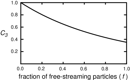
Figure 1: $C_{3}$ is the transfer function factor that accounts for the damping of the tensor power spectrum due to tensor anisotropic stress. The factor depends on the fraction $f$ of the background (critical) energy density contained in free-streaming relativistic particles. The figure plots this dependence for $0<f<1$.

The exact dependence of $C_{3}$ on $f$ is shown in Fig. 1. Note that, as $f$ varies between $0$ and $1$, the damping factor $C_{3}$ varies between $1.0$ and $0.35$. In particular, if we substitute $f=0.4052$, corresponding to 3 standard neutrino species,the damping factor $0.80313$ agrees with the results of numerical integrations Weinberg ; PritchKam . When the modes probed by the CMB re-enter the horizon, the temperature is relatively low (corresponding to atomic-physics energies), so we are fairly confident that neutrinos are the only free-streaming relativistic particles. But when the modes probed by laser interferometers re-enter the horizon, the temperature is much higher (above the electroweak phase transition, $T\sim 10^{7}$ GeV), so that the physics (and, in particular, the instantaneous free-streaming fraction $f$) is much more uncertain. Thus, laser interferometers offer the possibility of learning about the free-streaming fraction $f$ in the very early universe at temperatures between the inflationary and electroweak symmetry breaking scales.

Finally, although Weinberg and subsequent authors have concentrated on the tensor anisotropic stress due to a single fermionic species (the neutrino), it is straightforward to generalize the analysis to include a combination of species which (i) may each decouple at a different time and temperature, and (ii) may be an arbitrary mixture of bosons and fermions. We find that, as long as all of these free-streaming species decouple well before the modes of interest re-enter the horizon, then all of the results presented in this section are completely unchanged. In other words, in order to determine the behavior of the tensor mode function, one only needs to know one number — the total fraction $f$ of the critical density contained in free-streaming particles — even if the particles are a mixture of fermionic and bosonic species with different temperatures and decoupling times.

III.4 Equation-of-state corrections, $\delta w_{r}$

In this section, we consider various physical effects that cause the equation of state $w_{r}(z)$ to deviate from $1/3$ during the radiation-dominated epoch, and the corresponding modifications that these effects induce in the GWB transfer function. Some of these effects have been discussed previously by Seto and Yokoyama SetoYokoyama . The deviations

$$\delta w_{r}(z)=w_{r}(z)-1/3$$ (67)

primarily modify the transfer function through the redshift factor $(1+z_{k})$ that appears in $C_{1}$ [see Eqs. (49) and (50)]; through the horizon-crossing factor $C_{2}(k)$ [see Eq. (58)]; and through the phase shift $\phi_{k}$ [see Eq. (57)]. We consider here six physical effects which can produce these kinds of modifications of the transfer function.

First, deviations can be caused by mass thresholds in the early universe. Suppose that all particle species are described by equilibrium distribution functions. Then we can write $\rho$ and $p$ as

$$\rho = \frac{1}{2\pi^{2}}\sum_{i}g_{i}T_{i}^{4}\int_{x_{i}}^{\infty}\frac{(u^{2}-x_{i}^{2})^{1/2}}{{\rm exp}[u-y_{i}]\pm 1}u^{2}du,$$ (68a)

$$p = \frac{1}{6\pi^{2}}\sum_{i}g_{i}T_{i}^{4}\int_{x_{i}}^{\infty}\frac{(u^{2}-x_{i}^{2})^{3/2}}{{\rm exp}[u-y_{i}]\pm 1}du,$$ (68b)

where the $i$th species (with mass $m_{i}$, and $g_{i}$ internal degrees of freedom) is described by temperature $T_{i}$ and chemical potential $\mu_{i}$, and we have defined the dimensionless quantities $x_{i}\equiv m_{i}/T_{i}$ and $y_{i}\equiv\mu_{i}/T_{i}$ KolbTurner . In the denominator, the $+$ and $-$ signs are for fermions and bosons, respectively. Then the deviation $\delta w_{r}$ is given by the exact expression

$$\delta w_{r}=\sum_{i}\delta w_{r}^{(i)}$$ (69)

where

$$\delta w_{r}^{(i)}=-\frac{5}{\pi^{4}}\frac{g_{i}}{g_{\ast\rho}}\frac{T_{i}^{4}}{T^{4}}f(x_{i},y_{i})$$ (70)

represents the contribution from the $i$th species,

$$g_{\ast\rho}\equiv\sum_{i}g_{i}\frac{T_{i}^{4}}{T^{4}}\frac{15}{\pi^{4}}\int_{x_{i}}^{\infty}\frac{(u^{2}-x_{i}^{2})^{1/2}u^{2}}{{\rm exp}[u-y_{i}]\pm 1}du$$ (71)

represents the effective number of relativistic degrees of freedom, $T$ is conventionally chosen to be the photon temperature, and we have defined the function

$$f(x,y)\equiv x^{2}\int_{x}^{\infty}\frac{(u^{2}-x^{2})^{1/2}}{{\rm exp}[u-y]\pm 1}du.$$ (72)

For fixed $y_{i}$, note that $f(x_{i},y_{i})$ vanishes as $x_{i}$ goes to $0$ or $\infty$; and in between it has a fairly broad peak, with a maximum located at $x_{i}^{peak}$, and a peak value $f_{i}^{peak}=f(x_{i}^{peak},y_{i})$. In particular, when $y_{i}=0$, then the ordered pair $(x_{i}^{peak},f_{i}^{peak})$ is $(2.303,1.196)$ for bosons and $(2.454,1.125)$ for fermions. This makes sense: we expect $\delta w_{r}^{(i)}$ to vanish when $x_{i}\ll 1$ (since the species is relativistic) and when $x_{i}\gg 1$ (since the species is non-relativistic, and makes a negligible contribution to the energy density). In between, when $x_{i}\sim x_{i,peak}$, the $i$th species is cold enough to exhibit non-relativistic behavior, yet hot enough to contribute non-negligibly to the energy density.

Using the above equations, we can compute $\delta w_{r}(z)$ once we know $T_{i}(z)$ and $\mu_{i}(z)$. But let us estimate the size of the effect. As a species becomes non-relativistic, it produces a maximum equation-of-state deviation

$$\delta w_{r}^{(i)}=-\frac{5f_{i}^{peak}}{\pi^{4}}\frac{g_{i}}{g_{\ast\rho}}\frac{T_{i}^{4}}{T{}^{4}}$$ (73)

in the background equation of state. Furthermore, if $N_{s}$ different species (with the same temperature and similar masses) become non-relativistic at the same time, then (roughly speaking) the effect is multiplied by $N_{s}$ (since their $\delta w_{r}^{(i)}$’s add). Ultimately, the fractional correction $\delta w_{r}/w_{r}$ is model-dependent, but it can conceivably be as large as a few percent.

Second, deviations can be produced by a trace anomaly in the early universe. During the radiation-dominated epoch, the universe is dominated by highly relativistic particles whose masses may be neglected. Thus, each species is governed by a classical action that is conformally invariant at the classical level, leading to the usual conclusion that the stress-energy tensor is traceless and $w_{r}=1/3$. But conformal invariance is broken at the quantum level by interactions among the particles, so that $T_{\mu}^{\mu}\neq 0$. For example, for a quark-gluon plasma governed by SU($N_{c}$) gauge theory, with $N_{f}$ flavors, and gauge-coupling $g$, the equation of state correction is given (up to ${\cal O}(g^{5})$ corrections) by SU(Nc) ; grav_baryogen

$$\delta w_{r}=\frac{5}{18\pi^{2}}\frac{g^{4}}{(4\pi)^{2}}\frac{(N_{c}+\frac{5}{4}N_{f})(\frac{2}{3}N_{f}-\frac{11}{3}N_{c})}{2+\frac{7}{2}[N_{c}N_{f}/(N_{c}^{2}-1)]}.$$ (74)

Note that this effect can be non-negligible: for large gauge groups (i.e. large $N_{c}$) in the early universe (prior to the electroweak phase transition), the equation of state may $w_{r}$ may easily be reduced from $1/3$ by several percent, or more.

Third, deviations can be produced if the early universe behaves like a slightly imperfect fluid. The stress-energy tensor for an imperfect fluid contains (in addition to the usual perfect-fluid terms) three extra terms whose coefficients ($\chi$, $\eta$, and $\zeta$) represent heat conduction, shear viscosity, and bulk viscosity (see Weinberg WeinbergGR , Ch. 2.11). Of these dissipative effects, only the bulk viscosity term

$$\Delta T^{\mu\nu}=-\zeta(g^{\mu\nu}+U^{\mu}U^{\nu})U^{\lambda}_{\;\;;\lambda}$$ (75)

can contribute to the background evolution in an FRW universe (see Weinberg WeinbergGR , Chs. 15.10-15.11). This term modifies the continuity equation

$$\dot{\rho}=-3H(\rho+p)+9\zeta H^{2}=-3H\rho\Big{[}1+w-\frac{8\pi G\zeta}{H}\Big{]}$$ (76)

so that, as far as gravitational waves are concerned, the effective equation is corrected by

$$\delta w_{r}=-\frac{8\pi G\zeta}{H}.$$ (77)

Whereas the three effects discussed thus far produce small corrections to the equation of state, it is worth mentioning three other effects that can produce much larger deviations. The first example is a massive particle species that decouples from the thermal plasma before its abundance becomes negligible. Since its energy density falls as $a^{-3}$ (more slowly than the radiation density, which falls as $a^{-4}$), it can come to dominate the energy density of the universe before it decays (if its lifetime $\tau_{decay}$ is sufficiently long). In this case, $w$ drops to zero when the particle becomes dominant, and rises back to $w=1/3$ over a timescale given by the decay lifetime $\tau_{decay}$. Second, extra-dimensional physics typically modifies the effective 4-dimensional Friedmann equation. Such modifications which, from the standpoint of the GWB, can in some cases look like corrections to the effective radiation equation of state, are primarily constrained by the requirement that the Friedmann equation becomes sufficiently similar to the ordinary 4-dimensional Friedmann equation (with ordinary matter) by the time of BBN. Third, due to the weak coupling of the inflaton, the temperature at the start of the radiation dominated epoch (the reheat temperature) can be much lower than the energy scale at the end of inflation. In this case, laser interferometer scales might actually re-enter the horizon during the reheating epoch (before the start of radiation domination), when the equation of state was probably quite different from $w=1/3$. The actual equation-of-state depends on the details of the reheating process, but a commonly-discussed value is $w=0$, or some value in the range $0<w<1/3$ reheating . If $w=0$ during reheating, the corresponding modification of the GWB might be similar to the modification due to the long-lived massive relic discussed above.

Note that the first of these six processes can be expressed as a modification of $g_{\ast}$, and the effects on the transfer function can be computed using the methods discussed in Ref. SmithKamCoor . However, the other five cannot.

IV Discussion

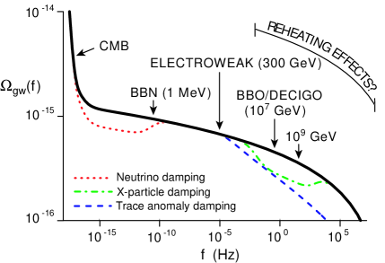
Figure 2: The black solid curve represents the present-day gravitational-wave energy spectrum, $\Omega_{gw}(f,\tau_{0})$, for the inflationary model $V(\phi)=(1/2)m^{2}\phi^{2}$. The red dotted curve shows the damping effect due to (three ordinary massless species of) free-streaming neutrinos. The green dot-dashed curve shows the damping effect which arises if free-streaming particles make up fifty percent of the background energy density at the time $\tau_{BBO}$ when the modes probed by BBO/DECIGO re-enter the horizon. As shown in the figure, the particles begin free-streaming sometime before $\tau_{BBO}$, and decay sometime after $\tau_{BBO}$, but prior to electroweak symmetry breaking. Finally, the blue dashed curve shows the effect of a conformal anomaly in the early universe that slightly reduces the equation of state from $w=0.33$ to $w=0.31$ above the electroweak phase transition. The spectrum will also be modified on comoving scales that re-enter the horizon during the reheating epoch after inflation; but the range of scales affected by reheating is unknown. Finally, note that the correlated BBO interferometer proposal claims a sensitivity that extends beyond the bottom of the figure (down to roughly $\Omega_{gw}\sim 10^{-17}$) in the frequency range from $10^{-1}$ Hz to $10^{0}$ Hz.

Fig. 2 illustrates some of the effects discussed in section III. In this figure, the solid black curve represents the present-day energy spectrum, $\Omega_{gw}(f,\tau_{0})$, generated by a particular inflationary model — namely, a quadratic potential $V(\phi)=(1/2)m^{2}\phi^{2}$. The red dotted curve illustrates the damping due to tensor anisotropic stress from free-streaming neutrinos. We have assumed that the free-streaming fraction is $f=0.4052$, which is the $f$ value for three standard neutrino species which decouple around the time of BBN. The green dot-dashed curve represents the damping due to tensor anisotropic stress from various particle species ($X$ particles) which begin free-streaming before the scales detected by BBO/DECIGO re-enter the horizon and then decay after the scales re-enter, but prior to the electroweak phase transition. As an example, we have assumed that the free-streaming fraction is $f=0.5$. Finally, the blue dashed curve represents damping due to a trace anomaly that is present above the electroweak scale. For illustration, we have assumed that this anomaly, through Eq. (74), reduces the equation of state from $w_{r}=1/3$ by $\delta w_{r}=-0.02$. This reduction may be achieved by various combinations of the number of colors $N_{c}$, the number of flavors $N_{f}$, and the gauge coupling $g$; but the point is that we have not chosen an unreasonable large value for $\delta w_{r}$, given the large gauge groups that are often theorized to be present at high energies.

The key point conveyed by Fig. 2 is that there are a variety of plausible post-inflationary effects that can produce rather large modifications of the gravitational-wave spectrum on laser-interferometer scales, without modifying the spectrum on CMB scales. This is tantalizing, since the modifications on laser-interferometer scales reflect the primordial dark age between the end of inflation and the electroweak phase transition, at energies beyond the reach of terrestrial particle accelerators.

Let us look ahead to future observations. First, as measurements of the scalar power spectrum improve, we will be restricted to considering inflationary models that match precisely the measured scalar perturbation spectrum on CMB scales. This is not enough to specify a unique model because there is a range of inflaton potentials whose scalar perturbation spectra are indistinguishable on CMB scales. For example, two such models are shown in Fig. 3.

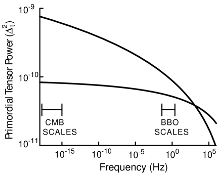
Figure 3: The precise predictions of the primordial tensor power spectrum for two inflationary models whose parameters have been chosen so that they make identical predictions for the scalar fluctuation amplitude and spectral index on CMB scales. The two models are the quartic monomial potential $V(\phi)=\lambda\phi^{4}$ (top), and the axion (or “natural inflation”) potential $V(\phi)=M_{I}^{4}[1+{\rm cos}(\phi/\mu)]$.

The two curves correspond to two different inflationary models whose parameters have been chosen so that they produce the same scalar amplitude and tilt on CMB scales, and match the observed scalar amplitude. From the figure, though, we see that their primordial tensor power spectra are distinguishable. The upper solid curve corresponds to the simple quartic monomial potential $V(\phi)=\lambda\phi^{4}$, and the lower solid curve corresponds to the axion (or “natural inflation” NaturalInflation ) potential $V(\phi)=M_{I}^{4}[1+{\rm cos}(\phi/\mu)]$.

Note that the two spectra “curve” significantly downward over the broad range of wavenumbers shown in Fig. 3, so that they are not well described by a power-law (straight-line) approximation over this range. In particular, a power-law extrapolation based on CMB measurements will give a fairly poor estimate of the real spectrum on laser-interferometer scales. In fact, since the real spectra tend to redden increasingly on smaller scales (i.e. as the end of inflation approaches), the CMB power-law extrapolation will tend to overestimate the tensor spectrum on laser-interferometer scales.

Second, note that the inflationary consistency relation (29) implies that a gravitational-wave spectrum with a larger tensor/scalar ratio $r$ on CMB scales also tends to have a “redder” (more negative) tilt $n_{t}$. For gravitational waves with detectably-large amplitudes on CMB scales, this leads to the “convergence effect” in Fig. 3: if two different inflationary models produce scalar perturbations with the same amplitude and tilt on large (CMB) scales, then their tensor spectra tend to approach and even cross one another on small (laser-interferometer) scales, as illustrated by the two solid black curves in Fig. 3. As a result, once one has measured the scalar and tensor perturbations on CMB scales, one expects the tensor spectrum on laser-interferometer scales to lie within a relatively narrow and predictable range.

This is both good news and bad news for laser-interferometer science. The bad news is that the convergence effect tends to make laser interferometers less effective at breaking any remaining degeneracies between inflationary models because their predictions for the tensor spectrum are so similar on small scales. The degree to which laser interferometers can break such degeneracies has been studied in SmithKamCoor . The good news is that the measurements can potentially provide a model-independent test of a key inflationary prediction: that the tensor spectrum observed at long wavelengths really does extend to small wavelengths, as expected from the consistency relation (29). Furthermore, precise laser-interferometer measurements can serve as sensitive probes of new post-inflationary physics that modifies the transfer function on small scales.

In this light, let us now imagine some time in the future in which we have successfully measured the tensor amplitude on CMB scales, and consider four possible outcomes of a laser-interferometer experiment (like BBO). First, suppose that BBO detects the gravitational-wave amplitude at the expected value, as exemplified in Fig. 3. This would be a quantitative confirmation of inflation generally, and of the inflationary consistency condition (29) in particular, since the large difference in wavenumber between CMB and laser-interferometer scales provides a large lever-arm to measure the tensor tilt $n_{t}$. It would also suggest an upper bound on the size of any exotic effects in the transfer function on laser-interferometer scales.

Second, suppose that BBO detects the gravitational-wave amplitude significantly below its expected value. Then the interpretation is less straighforward. On the one hand, we could interpret the suppression as being due to transfer-function effects, such as those discussed above. With this interpretation, the suppression would imply a rare opportunity to measure physical properties of the early universe, at temperatures above the electroweak scale, when the relevant modes re-entered the horizon. On the other hand, we could interpret the suppression to mean that inflation is more complicated than we expected: perhaps there is a feature in the inflaton potential which suppresses the primordial tensor spectrum on small scales relative to our expectations, or perhaps the consistency condition itself is violated (as it is in some multi-field models of inflation). Further measurements of the tensor spectrum at intermediate scales are needed to resolve this issue.

Third, suppose that BBO detects the gravitational-wave amplitude significantly above its expected value. At this point it is worth noting that virtually all of the transfer-function effects mentioned in section III (including tensor anisotropic stress, the late decay of a massive relic species, bulk viscosity, a conformal anomaly, or standard reheating with $w\leq 1/3$) suppress the gravitational-wave spectrum on small scales, relative to large scales. In order to enhance the spectrum on laser-interferometer scales, one must invoke an even more exotic effect, such as a reheating epoch with a low reheat temperature and an unusual equation of state ($w>1/3$); or the production of gravitational waves after inflation due to the collision of bubbles from a phase transition; or perhaps extra-dimensional physics.

Fourth, suppose that BBO detects nothing at all. This would most likely indicate a fundamental problem with inflation, since an period of accelerating expansion produces a broad and nearly-flat spectrum of primordial tensor perturbations quite generically (regardless of the particular model that drives inflation). One way out of this conclusion would be to invoke an extreme suppression effect in the transfer function on BBO scales — e.g. due to a reheating epoch with equation of state $w=0$ and a reheat temperature well below $10^{7}$ GeV. Determining which interpretation is correct would require digging deeper, with more sensitive experiments on BBO scales.

References

- (1) A. H. Guth, Phys. Rev. D 23, 347 (1981); A. D. Linde, Phys. Lett. B 108, 389 (1982); A. Albrecht and P. J. Steinhardt, Phys. Rev. Lett. 48, 1220 (1982).
- (2) L. P. Grishchuk, Sov. Phys. JETP 40, 409 (1975); A. A. Starobinsky, JETP Lett. 30, 682 (1979).
- (3) R. K. Sachs and A. M. Wolfe, Astroph. J. 147, 73 (1967); A. G. Doroshkevich, I. D. Novikov and A. G. Polnarev, Sov. Astron. 21, 529 (1977).
- (4) V. A. Rubakov, M. V. Sazhin and A. V. Veryaskin, Phys. Lett. B 115, 189 (1982); R. Fabbri and M. d. Pollock, Phys. Lett. B 125, 445 (1983); L. F. Abbott and M. B. Wise, Nucl. Phys. B 244, 541 (1984); A. A. Starobinsky, Sov. Astron. Lett. 11, 133 (1985).
- (5) A. G. Polnarev, Sov. Astron. 29, 607 (1985).
- (6) M. Kamionkowski, A. Kosowsky and A. Stebbins, Phys. Rev. Lett. 78, 2058 (1997) [arXiv:astro-ph/9609132]; Phys. Rev. D 55, 7368 (1997) [arXiv:astro-ph/9611125].
- (7) U. Seljak and M. Zaldarriaga, Phys. Rev. Lett. 78, 2054 (1997) [arXiv:astro-ph/9609169]; M. Zaldarriaga and U. Seljak, Phys. Rev. D 55, 1830 (1997) [arXiv:astro-ph/9609170].
- (8) R. Weiss et al, Task Force On Cosmic Microwave Research, www.science.doe.gov/hep/TFCRreport.pdf
- (9) M. S. Turner, Phys. Rev. D 55, 435 (1997) [arXiv:astro-ph/9607066].
- (10) T. L. Smith, M. Kamionkowski and A. Cooray, arXiv:astro-ph/0506422.
- (11) N. Seto, S. Kawamura and T. Nakamura, Phys. Rev. Lett. 87, 221103 (2001) [arXiv:astro-ph/0108011].
- (12) E. S. Phinney, private communication (2005).
- (13) see the URL:universe.nasa.gov/program/bbo.html.
- (14) C. Ungarelli, P. Corasaniti, R. A. Mercer and A. Vecchio, Class. Quant. Grav. 22, S955 (2005) [arXiv:astro-ph/0504294].
- (15) J. Crowder and N. J. Cornish, Phys. Rev. D 72, 083005 (2005) [arXiv:gr-qc/0506015].
- (16) M. S. Turner, M. J. White and J. E. Lidsey, Phys. Rev. D 48, 4613 (1993) [arXiv:astro-ph/9306029].
- (17) S. Bashinsky, arXiv:astro-ph/0505502.
- (18) S. Weinberg, Phys. Rev. D 69, 023503 (2004) [arXiv:astro-ph/0306304].
- (19) D. A. Dicus and W. W. Repko, Phys. Rev. D 72, 088302 (2005) [arXiv:astro-ph/0509096].
- (20) J. R. Pritchard and M. Kamionkowski, Annals Phys. 318, 2 (2005) [arXiv:astro-ph/0412581].
- (21) L. P. Grishchuk and Y. V. Sidorov, Class. Quant. Grav. 6, L155 (1989); L. P. Grishchuk and Y. V. Sidorov, Phys. Rev. D 42, 3413 (1990).
- (22) B. Allen, E. A. Flanagan and M. A. Papa, Phys. Rev. D 61, 024024 (2000) [arXiv:gr-qc/9906054].
- (23) A. Albrecht, P. Ferreira, M. Joyce and T. Prokopec, Phys. Rev. D 50, 4807 (1994) [arXiv:astro-ph/9303001].
- (24) V. F. Mukhanov, H. A. Feldman and R. H. Brandenberger, Phys. Rept. 215, 203 (1992).
- (25) J. Maldacena, JHEP 0305, 013 (2003) [arXiv:astro-ph/0210603].
- (26) J. M. Bardeen, Phys. Rev. D 22, 1882 (1980).
- (27) H. Kodama and M. Sasaki, Prog. Theor. Phys. Suppl. 78, 1 (1984).
- (28) N. D. Birrell and P. C. W. Davies, Quantum Fields in Curved Space (Cambridge University Press, Cambridge, England, 1982).
- (29) H. V. Peiris et al., Astrophys. J. Suppl. 148, 213 (2003) [arXiv:astro-ph/0302225].
- (30) K. S. Thorne, in 300 Years of Gravitation, edited by S. Hawking and W. Israel (Cambridge University Press, Cambridge, England, 1987), pp. 330-458.
- (31) C. W. Misner, K. S. Thorne and J. A. Wheeler, Gravitation (W. H. Freeman and Company, San Francisco, United States, 1973).
- (32) N. Seto and J. Yokoyama, J. Phys. Soc. Jap. 72, 3082 (2003) [arXiv:gr-qc/0305096].
- (33) E. W. Kolb and M. S. Turner, The Early Universe, Addison-Wesley, 1990.
- (34) K. Kajantie, M. Laine, K. Rummukainen and Y. Schroder, Phys. Rev. D 67, 105008 (2003) [arXiv:hep-ph/0211321].
- (35) H. Davoudiasl, R. Kitano, G. D. Kribs, H. Murayama and P. J. Steinhardt, Phys. Rev. Lett. 93, 201301 (2004) [arXiv:hep-ph/0403019].
- (36) S. Weinberg, Gravitation and Cosmology, John Wiley & Sons, Inc. (1972).
- (37) D. I. Podolsky, G. N. Felder, L. Kofman and M. Peloso, arXiv:hep-ph/0507096.
- (38) K. Freese, J. A. Frieman and A. V. Olinto, Phys. Rev. Lett. 65, 3233 (1990).