Evolution of Galactic Nuclei. I. orbital evolution of IMBH

Abstract

Resent observations and theoretical interpretations suggest that IMBHs (intermediate-mass black hole) are formed in the centers of young and compact star clusters born close to the center of their parent galaxy. Such a star cluster would sink toward the center of the galaxy, and at the same time stars are stripped out of the cluster by the tidal field of the parent galaxy. We investigated the orbital evolution of the IMBH, after its parent cluster is completely disrupted by the tidal field of the parent galaxy, by means of large-scale $N$-body simulations. We constructed a model of the central region of our galaxy, with an SMBH (supermassive black hole) and Bahcall-Wolf stellar cusp, and placed an IMBH in a circular orbit of radius 0.086pc. The IMBH sinks toward the SMBH through dynamical friction, but dynamical friction becomes ineffective when the IMBH reached the radius inside which the initial stellar mass is comparable to the IMBH mass. This is because the IMBH kicks out the stars. This behavior is essentially the same as the loss-cone depletion observed in simulations of massive SMBH binaries. After the evolution through dynamical friction stalled, the eccentricity of the orbit of the IMBH goes up, resulting in the strong reduction in the merging timescale through gravitational wave radiation. Our result indicates that the IMBHs formed close to the galactic center can merge with the central SMBH in short time. The number of merging events detectable with DECIGO is estimated to be around 50 per year. Event rate for LISA would be similar or less, depending on the growth mode of IMBHs.

1. Introduction

Recent observations (Matsumoto et al. 2001; Matsushita et al. 2000) suggested that intermediate-mass black holes (IMBHs) exist in some starburst galaxies. The first such object, M82 X-1 (the brightest source in Figure 1 of Matsumoto et al. (2001)) lays 200pc off the dynamical center of M82, and has the estimated minimum mass of 700 $M_{\odot}$. Several scenarios have been proposed for the formation of this object (Ebisuzaki et al. 2001; Miller & Hamilton 2002; Kawakatu 2002; Taniguchi et al. 2000). Both Ebisuzaki et al. and Miller and Hamilton argued that IMBHs are formed through stellar dynamical process and merging. The main difference between them is simply in the time at which the merging occurs. Ebisuzaki et al. assumed that most of merging process occurred while participants were main-sequence stars. On the other hand, Miller and Hamilton assumed that the IMBH grew through merging of smaller black holes.

Which of the two processes actually occur depends mainly on the initial thermal relaxation time of the cluster. Portegies Zwart et al. (2004) showed, using $N$-body simulations, that the runaway merging of massive star occurs if the initial relaxation time of the star cluster is less than 4 Myrs, which is of the order of the lifetime of massive stars. The compact star cluster MGG-11 (McCrady et al. 2003), which coincides with the location of M82 X-1, has the estimated relaxation time of 3 Myrs. On the other hand, the relaxation time of MGG9, which is more massive than MGG11, is significantly longer. This difference is consistent with the existence and nonexistence of IMBHs in MGG-11 and 9, respectively. In the case of the scenario by Miller and Hamilton, the growth timescale would be much longer, and it is hard to explain why any IMBH can exist in a young cluster like MGG-11.

Compared to the relaxation time of typical globular clusters, which is $10^{8\sim 9}$ yrs, the relaxation time of a few Myrs might sounds extremely short. However, for young clusters, such short relaxation time is not unusual. For example, Arches and Quintuplet clusters, whose estimated ages are around 1-5 Myrs years, have the estimated relaxation time of 12M years (Portegies Zwart et al. 2002). Star clusters R136 in LMC and Westerlund 1 in our galaxy are other examples of such young compact clusters.

If the formation of IMBHs is not a rare event in young and compact clusters, two questions naturally arise. What is the final fate of the IMBH and its parent cluster, and whether or not it is related to the growth of the central black hole of the parent galaxy. The star cluster itself evolves through internal thermal relaxation, tidal truncation, and dynamical friction, much in the same way as globular clusters evolve. The main difference is again that the timescale is much shorter. For example, if there is a cluster with mass $10^{5}M_{\odot}$ at the distance of 30 pc from the center of our Galaxy, the dynamical friction timescale would be

$$t_{\rm fric} \simeq \frac{2.38\times 10^{8}}{\ln\Lambda}\left(\frac{r}{30{\rm pc}}\right)^{2}$$ (1)

$$\left(\frac{\sigma}{100{\rm km~{}s^{-1}}}\right)\left(\frac{10^{5}M_{\odot}}{M_{c}}\right)yr~{},$$

where $\sigma$ is a velocity dispersion and $M_{c}$ is the mass of the cluster.

As the cluster sinks toward the center of the parent galaxy, the tidal field of the galaxy becomes stronger. As a result, the cluster loses mass, and eventually becomes completely disrupted, leaving the IMBH orbiting around the central SMBH. IRS13E (Maillard et al. 2004) looks like such a remnant cluster, composed of a single IMBH and several stars still bound to it (Portegies Zwart et al. 2005) IRS13E is located at 4 arcsec ($\sim$0.16pc) from Sgr A^∗. It appears as a cluster of seven individual stars within a projected diameter of $\sim$ 0.5 arcsec (0.02 pc). All these sources have a common westward proper motion, indicating that they are bound (at least six of them). The types of stars imply that it is a young star cluster with the age of a few Myrs. To keep these stars bound, the total gravitational mass of IRS13E must exceed $1300M_{\odot}$, about one order of magnitude larger than the estimated total mass of visible stars. One natural interpretation is that IRS13E is a remaining core of much more massive star cluster, with an IMBH of $\sim 1300M_{\odot}$.

In this paper, we consider the orbital evolution of an IMBH after its parent cluster is completely disrupted. The main question is the merging timescale of the IMBH and the central SMBH. In the case of a massive BH binary, which forms when two galaxies each with a central massive BH merge, the merging timescale has been the area of active research since the pioneering work by Begleman, Blandford, & Rees (1980). In this case, the result of recent large-scale $N$-body simulations (Makino & Funato 2004) suggests that the merging timescale is much longer than the Hubble time. They demonstrated that the evolution timescale of the BH binary is proportional to the relaxation time of the parent galaxy, as suggested by Begleman, Blandford, & Rees (1980). This conclusion is different from the results of previous simulations (Quinlan & Hernquist 1997; Makino 1997; Milosavljevi${\rm\acute{c}}$ & Merritt 2001; 2003; Chatterjee et al. 2003), but the difference is mostly due to the limitation in the number of particles in previous simulations. Szell & Merritt (2005) and Berczik et al. (2005) obtained similar results as Makino & Funato (2004), albeit with somewhat smaller number of particles.

However, we cannot directly apply these result to the case of an SMBH-IMBH binary, because of its very large mass ratio. In the case of SMBH-SMBH binary, the binary need to interact with the field stars with the total mass comparable to that of the total mass of the binary to change its internal orbital parameters significantly. Thus, the loss-cone depletion occurs when the binary ejected out the mass comparable to its mass, and the structure outside the loss cone region is self-gravitating. In the case of SMBH-IMBH binary, the IMBH orbit can evolve by interacting with the mass comparable to the IMBH mass which is several orders of magnitude smaller than the SMBH mass. Thus, loss cone depletion can occur when the IMBH ejected out the central stellar mass comparable to the IMBH mass, and the gravitational potential of this region, or actually of the region much further out, is dominated by the potential of the central BH. Thus, unlike the case of SMBH-SMBH binary, we need to study the evolution of a highly unequal mass binary, in the distribution of stars which are all bound to the primary component of the binary.

The organization of the paper is as follows. In §2, we describe the numerical method and the initial conditions we used. In §3 and §4, we describe the result of the simulations. Summary and discussion are presented in §5.

2. Initial models and numerical methods

2.1. Initial Models

The goal of this paper is to study the orbital evolution of an IMBH in the stellar distribution where the gravitational potential of the central SMBH dominates. As the background stellar distribution, we adopt the standard $\rho\propto r^{-7/4}$ cusp (Bahcall & Wolf 1976). One practical problem with this distribution is that the total mass would be infinity if the density profile is given by this single power law. In addition, such a model is physically unacceptable, since the basic assumption for the Bahcall-Wolf cusp is that the gravitational potential is dominated by that of the central BH.

In order to construct a model with central density slope of $-7/4$ and finite mass, we use Tremaine’s $\eta$-model with central BH (Tremaine et al. 1994), with one modification. The original $\eta$-model has the outer slope of $-4$. We constructed the model with outer slope of $-5$, just to make the mass in the outer region smaller.

The density distribution of our modified model is given by

$$\rho_{\eta}(r)=\frac{\eta}{4\pi}\frac{M_{\eta}r_{0}^{2}}{r^{3-\eta}(r_{0}^{2}+r^{2})^{\eta/2+1}}~{},~{}0<\eta\leq 3,$$ (2)

where $M_{\eta}$ is the total mass of field stars and $r_{0}$ is the scale length. The model with $\eta=5/4$ correspond to profile $\rho\propto r^{-7/4}$, and we use it in this paper.

In order to construct an $N$-body model in dynamical equilibrium, we need to construct the distribution function (DF). We could obtain DF at least numerically by solving the Abel integral equation. However, since what we need is a model with an inner power-law cusp and some outer cutoff, it would be an overkill to obtain a distribution function which exactly satisfies equation (2). So we approximate DF by the following formula.

$$f(\epsilon)=f_{0}(\epsilon)^{7/2}\left(\epsilon_{0}^{s}+\epsilon^{s}\right)^{-\frac{\eta+2}{s}}~{},$$ (3)

where $\epsilon\equiv-E$,

$$\epsilon_{0}=\left(\frac{f_{1}}{f_{0}}\right)^{-1/(\eta+2)}~{},$$ (4)

$$f_{0}=\frac{\eta M_{\eta}\Gamma(4-\eta)}{2^{7/2}\pi^{5/2}M_{S}^{3-\eta}\Gamma(5/2-\eta)},$$ (5)

and

$$f_{1}=\frac{8\sqrt{2}}{7\pi^{3}}{\eta M_{\eta}}~{}.$$ (6)

DF of this form gives a correct asymptotic behavior for both $\epsilon\rightarrow\infty$ and $\epsilon\rightarrow 0$. This formula has one adjustable parameter $s$. We chose $s=5$ after some numerical tests.

We generated the initial $N$-body model in the following two steps. First, we generate positions of $N$ particles so that the density distribution obeys equation (2). Then we assign the velocity to each particle, so that the velocity distribution at the point of particle is consistent with the DF given in equation (3). Since the DF we used is an approximate solution, the constructed $N$-body model is not in an exact dynamical equilibrium. However, as we will see in §2.3, our initial model is in pretty good dynamical equilibrium.

We chose the system of units in which the total mass of the system and gravitational constant are both unity and the total binding energy of the system is $-1/4$. We set the mass of SMBH to be $M_{S}=0.5$, that of the IMBH $M_{I}=5\times 10^{-4}$. The mass of the stellar distribution is therefore $0.4995$. The stellar mass inside the radius $r$ is

$$M_{\eta}(r)=M_{\eta}\frac{r^{\eta}}{(r_{0}^{2}+r^{2})^{\eta/2}}.$$ (7)

For the above choice of the system of units, $r_{0}\simeq 2.39$. When constructing the initial stellar distribution, we exclude the stars with periastron distance less than $10^{-3}$, to avoid numerical problem.

Figure 1.— Cumulative mass distribution of Our Galaxy obtained from stellar and gas dynamics and that of our and Genzel 2000 models. Triangles denote mass estimates from the gas dynamics (Guesten et al. 1987). Crosses, circles and squares denote the isotropic mass modeling of Genzel et al. (1996; 1997; 2000). Dashed curve is the mass model by Genzel et al. (2000), whose stellar distribution is $\rho(r)=\rho_{0}[1+(r/r_{0})^{2}]^{-\alpha/2}$, of $\rho_{0}=3.5\times 10^{6}M_{\odot}$, $r_{0}=0.17$pc and $\alpha=1.8$. Solid curve is our model, drawn using single power-law mass distribution with $\rho\propto r^{-7/4}$.

To convert the timescale obtained in our simulations to the physical timescale, we need to define conversions between our system of units and real physical units. We use unit mass $M=6.0\times 10^{6}M_{\odot}$, unit length $R=0.86$pc, resulting in the unit time of $T=4.6\times 10^{3}$yrs. Mass and length units are chosen so that the stellar mass inside the radius 0.7pc (assuming that the single power law with $-7/4$ slope continues to that radius) is $7.3\times 10^{5}M_{\odot}$ (Genzel et al. 2000). Figure 1 shows the mass distribution for our model (assuming single power-law density), the model by Genzel et al. (2000), and observational data. Note that our model is within the observational error bars and practically indistinguishable with the model by Genzel et al. (2000).

The IMBH particle is placed in a circular orbit at the radius 0.1 (0.086pc in physical units). Its mass is $3000M_{\odot}$.

We performed four runs with different number of field particles (models A1 to A4 of table 1). The mass of a field particle in model A4 is 30 $M_{\odot}$, which is not too far from the mass of real stars (whatever they are) in this region.

In table 1, models B1 to B4 were prepared to study the evolution of the IMBH after it approaches to less than 0.01 pc to the SMBH. For these models, we used $r_{0}$ much smaller than that is used for model Ax, to reduce the total number of stars. We used $r_{0}=0.1$ and placed the IMBH at $r=0.01$, so that the stellar distribution at the initial position of IMBH is still the power law with slope $-7/4$. The total stellar mass is $8.9\times 10^{-3}$, or about 20 times the IMBH mass. Results of Bx models will be discussed in §4. Mass of a field particle in model B4 is 3 $M_{\odot}$, which is of the same order with that of real stars in this region. Thus, two-body relaxation effect in this model is essentially the same as what would occur in the real galactic center.

We made models C1 and C2 to test the effect of softening parameters (see in §2.2) and D1 and D2 to test the validity of the initial model and relaxation effect (see §2.3).

2.2. Hardware and Numerical Integration Method

For all calculations, we used simple direct-summation algorithm and fourth-order Hermite scheme integrator with individual (block) time step (Makino & Aarseth 1992).

For the calculation of gravitational forces from field particles (to both the field particle and black holes), we used the GRAPE-6 (and -6A) of Tokyo University, a special purpose computer for $N-$body simulation (Makino et al. 2003; Fukushige et al. 2005). The calculation of the forces from black holes was done on the host computer to maintain sufficient accuracy. We did not include any relativistic effects and treated BH particle as massive Newtonian particle.

In our calculation, we did not use regularization technique to keep the calculation code simple. Thus, we need to apply softening parameters for gravitational interactions between particles. We use four different softening lengths, for BH-BH, SMBH-star, IMBH-star, and star-star interactions.

For SMBH-IMBH interaction, we apply zero softening. They cannot easily come close enough to each other for the numerical difficulty to occur. If such close encounter occurs, the timescale of orbital evolution through gravitational wave radiation becomes short enough so that our pure Newtonian treatment is not really valid.

The softening for BH-star interaction should be determined with some care, since close encounters do occur and too large softening can affect the orbital evolution of the IMBH. For the softening of SMBH-star interaction, we used $\epsilon_{S\mbox{-}s}=10^{-4}$ and $10^{-6}$ in Ax and Bx runs, respectively. These values are chosen so that the effect of softening is small enough for stars at the radius comparable to that of the IMBH.

For IMBH-star interaction, we chose the softening so that it is smaller than 90-degree turnaround distance by at least two orders of magnitude at the initial condition. As the IMBH approaches to SMBH, the velocity dispersion becomes larger, the difference between the softening length and the 90-degree turnaround distance becomes smaller, but it was always kept significantly larger than 1.

Table 1 List of parameters for the simulations in this paper.

Run	$N_{fs}$	${M_{I}/m_{\ast}}$	$r_{\rm I}$	$\epsilon_{S\mbox{-}s}$	$\epsilon_{I\mbox{-}s}$	$\epsilon_{s\mbox{-}s}$
A1	9990	10.0	0.1	$10^{-4}$	$10^{-6}$	$10^{-4}$
A2	19980	20.0	0.1	$10^{-4}$	$10^{-6}$	$10^{-4}$
A3	39960	40.0	0.1	$10^{-4}$	$10^{-6}$	$10^{-4}$
A4	99900	100.0	0.1	$10^{-4}$	$10^{-6}$	$10^{-4}$
B1	1795	100.0	0.01	$10^{-6}$	$10^{-8}$	$10^{-4}$
B2	3589	200.0	0.01	$10^{-6}$	$10^{-8}$	$10^{-4}$
B3	7177	400.0	0.01	$10^{-6}$	$10^{-8}$	$10^{-4}$
B4	17942	1000.0	0.01	$10^{-6}$	$10^{-8}$	$10^{-4}$
C1	99900	100.0	0.1	$10^{-4}$	$10^{-6}$	$10^{-3}$
C2	99900	100.0	0.1	$10^{-4}$	$10^{-6}$	$10^{-5}$
D1	10000	–	–	$10^{-4}$	–	$10^{-4}$
D2	100000	–	–	$10^{-4}$	–	$10^{-4}$

The criterion of the softening for star-star interaction is more complicated. Since the ”stars” in our model is still significantly heavier than real stars (assuming we know what the mass of real stars in this region), it is desirable to use large softening to reduce the relaxation effect. On the other hand, the softening should be small enough not to affect the distribution of stars. For most of runs we used the softening length of $10^{-4}$. As the test calculations, we performed two runs with $\epsilon_{s\mbox{-}s}=10^{-3}$ and $10^{-5}$, (runs C1 and C2). As will be discussed in §2.3, these runs gave essentially the same results are the standard run (run A4). So we used $\epsilon_{s\mbox{-}s}=10^{-4}$ for all other runs. Table 1 also gives the softening parameters used.

The largest calculation (model B4) took about five weeks on a single-host, single processor-board GRAPE-6 system with a peak speed of 1 T-flops. For all calculations, the total energy is conserved to better than 0.5% for all Ax, Cx and Dx runs. For models Bx the total energy conservation is shown in Figure 13.

2.3. Stability and relaxation effect

Figure 2.— Radial density profiles at times $T=0$ and $1000$ for runs D1 and D2.

Figure 3.— Lagrangian radii around SMBH for runs D1 and D2. From bottom to top, the radii enclose $5\times 10^{-5},$ $10^{-4},2\times 10^{-4},5\times 10^{-4},$ $10^{-3},2\times 10^{-3},5\times 10^{-3},$ 0.01 and 0.02 of the unit mass.

As described in §2.1 our initial model is not in exact dynamical equilibrium. In addition, the system would evolve through two-body relaxation even if the initial model is in exact dynamical equilibrium. To see these effects, we performed two test calculations (models D1 and D2), where we let the system without the IMBH to evolve for 1000 time units. Figures 2 and 3 show the result.

We can see that the density profiles are practically unchanged, and that Lagrangian radii do not show any systematic evolution.

2.4. Effect of star-star softening

As we discussed in §2.2, the choice of softening for star-star interaction might have some unpredictable effect on the evolution of the orbit of the IMBH. To see if there is any such effect, we performed two runs, models C1 and C2, which started from the same initial condition as model A4 but with different values of $\epsilon_{s\mbox{-}s}$.

Figure 4.— Evolution of the semi-major axis and the eccentricities of the black hole binary. Dotted, dashed, and solid curves denote $\epsilon_{s\mbox{-}s}=10^{-3}$, $10^{-5}$ and $10^{-4}$, respectively.

The result is shown in figure 4. There is no systematic difference among these three runs. So we can conclude that the choice of $\epsilon_{s\mbox{-}s}$ has no significant effect on the result.

3. Results

3.1. Hardening Rate

Figure 5.— Evolution of the semi-major axis of the IMBH. Dotted, dash-dotted, dashed, and solid curves are the results of models A1-4. Thin curve shows the theoretical curve calculated equation (16).

Figure 5 shows the time evolution of the semi-major axis of the IMBH, or the SMBH-IMBH binary. Here and hereafter, we refer to orbital elements and other quantities of IMBH-SMBH binary as those of the IMBH, for simplicity. The semi-major axis of the IMBH is given by

$$a=-\frac{GM_{S}M_{I}}{2E_{b}}~{},$$ (8)

where $E_{b}$ is the binding energy of the IMBH

$$E_{b}=\frac{1}{2}\mu V_{b}^{2}-\frac{GM_{S}M_{I}}{r}.$$ (9)

Here, $V_{b}$ is the relative velocity of the two BHs and $\mu$ is the reduced mass defined as

$$\mu\equiv M_{\rm S}M_{\rm I}/(M_{\rm S}+M_{\rm I}).$$ (10)

From figure 5, we can see that the orbital evolution of the IMBH is practically independent of the number of stars in the parent galaxy. In all models, the IMBH is much more massive than the field stars. So this result is not surprising.

The thin solid curve of in figure 5 is the theoretical prediction for the evolution of the IMBH orbit, obtained using standard dynamical friction formula (Binney & Tremaine 1987)

$$\frac{dV_{b}}{dt}=-\frac{4\pi\ln\Lambda G^{2}\rho M_{I}}{V_{b}^{2}}G(X).$$ (11)

where

$$G(X)={\rm erf}(X)-\frac{2X}{\sqrt{\pi}}\exp(-X^{2}),$$ (12)

and

$$X\equiv V_{b}/(\sqrt{2}\sigma).$$ (13)

Here $\sigma$ is the velocity dispersion and we used the circular velocity $V_{b}=\sqrt{GM_{S}/a}$ as the velocity of the IMBH. We used $\ln\Lambda=8$ here. For the calculation of dynamical friction in inhomogeneous background distribution, it has been suggested that taking the outer cutoff of Coulombs logarithm to the distance of the object from the center of the parent stellar system gives good estimate (Hashimoto et al. 2003). The lower cutoff is 90-degree turnaround distance, which is given by

$$r_{c}\sim a\frac{M_{I}}{M_{S}}=10^{-3}a.$$ (14)

Thus, we have $\log\Lambda\sim 7$ independent of the location of the IMBH. Using equation (2), equation (11) can be rewritten as follows

$$\frac{da}{dt} \simeq \frac{10.7\ln\Lambda G^{1/2}\rho_{0}M_{I}a^{3/4}}{{M_{S}}^{3/2}}~{},$$ (15)

where $\rho_{0}$ is the stellar mass density at $r=1$ and we assume the circular motion so that we used $a=r$.

We chose $X=1$ here. This differential equation has the analytic solution given by

$$a=a_{0}\left(\frac{T_{0}-T}{T_{0}}\right)^{4}~{},$$ (16)

where

$$T_{0}=\frac{0.37~{}a_{0}^{1/4}~{}M_{S}^{3/2}}{\ln\Lambda~{}G^{1/2}~{}\rho_{0}M_{I}}~{}.$$ (17)

We can see that the agreement between the theoretical prediction and numerical result is pretty good, at least for the early period ($T<600$). In the later phase, it seems the numerical results show the slowing down of the evolution.

Figure 6.— Hardening rate $\beta$ in equation (18), plotted as a function of semi-major axis $a$ at time $(t_{0}+\Delta t/2)$, for runs A1-4. Thin curve shows the theoretical prediction in equation (15).

To see the difference between the theoretical prediction and numerical results more clearly, we calculated the hardening rate $\beta$, defined as

$$\beta=-\frac{\Delta a}{\Delta t}.$$ (18)

Here $\Delta(1/a)=|a_{1}-a_{0}|$, where $a_{1}$ and $a_{0}$ are the semi-major axis of the IMBH at times $t=t_{0}$ and $t_{0}+\Delta t$, respectively. We use $\Delta t=100$ for all values of $t_{0}$. Figure 6 shows the result. The agreement between the theoretical prediction and numerical results is fairly good for $a>0.01$. For $a<0.01$, numerical result gives the hardening rate smaller than the theoretical prediction, and the difference becomes larger as $a$ becomes smaller.

Figure 7.— Time evolution of Lagrangian radii of field stars. From bottom to top, the curves show the radii containing the mass $5\times 10^{-5}$ ($10^{-4}$ of the stellar mass), $10^{-4},2\times 10^{-4},5\times 10^{-4},$ $10^{-3},2\times 10^{-3},5\times 10^{-3},$ 0.01 and 0.02. Four panels show the result of runs A1 through A4 (model names are shown in panels). Thick solid curves show the semi-major axis of the IMBH.

A natural explanation of this slowing down is the loss-cone depletion, similar to what happens in the case of massive BH binaries. Figures 7 show the Lagrangian radii of field stars. We used the position of SMBH as the coordinate center. We can see that as the IMBH sink toward the center, the Lagrangian radius corresponding to the position of the IMBH starts to expand. For example, in the case of model A4, the radius enclosing the mass of $2\times 10^{-3}$ (fourth curve from the top) starts to expand at around $t=400$, which is the time the IMBH semi-major axis crosses that radius. Radii enclosing smaller masses show similar tendency, though the expansion is faster for radii with smaller mass.

Since the expansion of a Lagrangian radius starts when the IMBH reaches that radius, we can conclude that this expansion is due to the back reaction of dynamical friction to the IMBH. Thus, when the stellar mass inside the IMBH semi-major axis becomes comparable to the IMBH mass, the effect of back reaction becomes significant. Stellar mass inside $r=0.01$ is about 0.1% of the total stellar mass, which is about the same as the IMBH mass. Thus, when the IMBH reaches the radius 0.01, the effect of the IMBH to the stellar distribution becomes significant, and number density of field stars is reduced. This is the reason why the hardening rate becomes smaller when $a$ reaches 0.01.

3.2. Change of the distribution of field stars

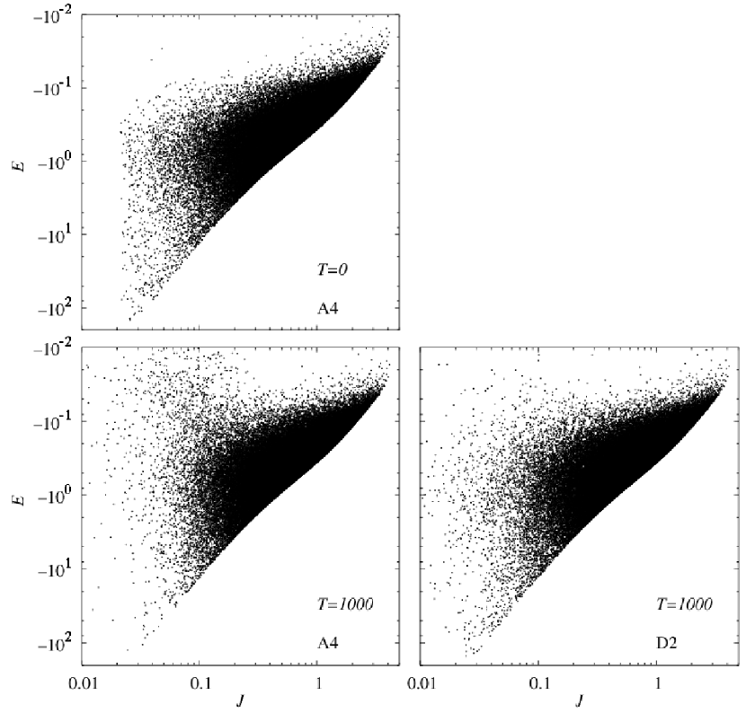
Figure 8.— Distribution of the field stars in the $(J,E)$ plane at time $T=0$ for run A4 and those at $T=1000$ for runs A4 and D2.

Figures 8 show the distribution of the field stars in the $(J,E)$ plane, for run A4 and D2 at $T=0$ and 1000. Here, $E$ and $J$ are the specific binding energy and specific total angular momentum of field stars. We take the center of mass of SMBH-IMBH binary as the origin tocalculate $E$ and $J$.

Note that we excluded field particles with the periastron distance to SMBH less than $10^{-3}$ when we constructed the initial condition. The left-hand-side cutoff in the distribution (at around $J=0.02$) is due to this exclusion.

When we compare the panels, it is clear that field particles with small $J$ ($J<0.03$) and large negative $E$ ($E<-10$) are depleted in model A4, while no such tendency is visible for model D2 (without IMBH). These particles are kicked out to high-energy, low-angular-momentum orbits by interaction with the IMBH.

There are many particles in the area $J<0.1$ and $E>-0.2$ in $T=1000$ panel for run A4, while these are not in model D2. It is clear that these particles were kicked out by interaction with the IMBH from the small $J$ and large negative $E$ region.

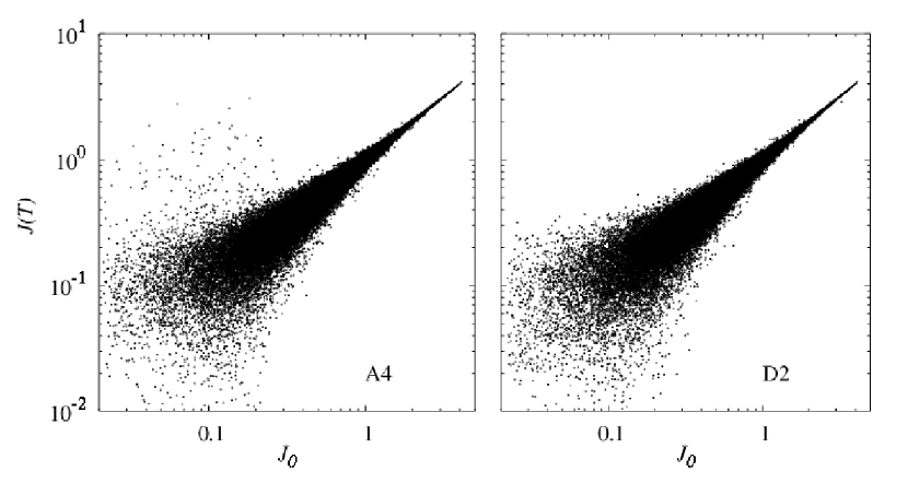
Figure 9.— Distribution of the field stars in the ($J_{0},J(T)$) planes for runs A4 and D2. $J_{0}$ is the initial specific total angular momentum and $J(T)$ is that at the time $T=1000$.

Figures 9 show the initial and final ($T=1000$) total angular momentum of stars for runs A4 and D2. In the case of run A2, we can see that a fair number of particles which initially have small $J$ ($J<0.2$) got much larger $J$. It indicates that field particles are kicked out by the IMBH. The dispersion in the case of run D2 is purely due to the two-body relaxation.

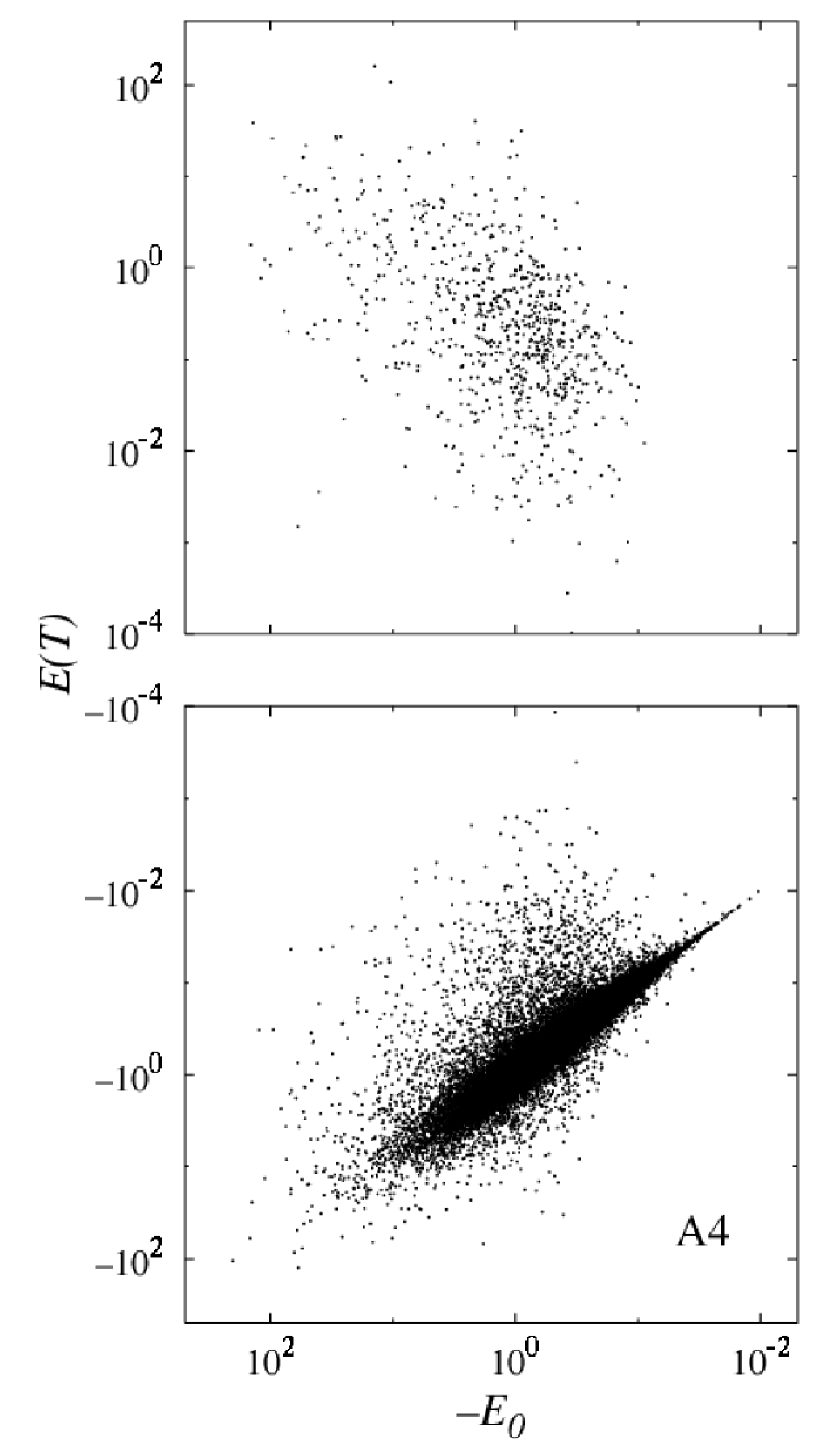
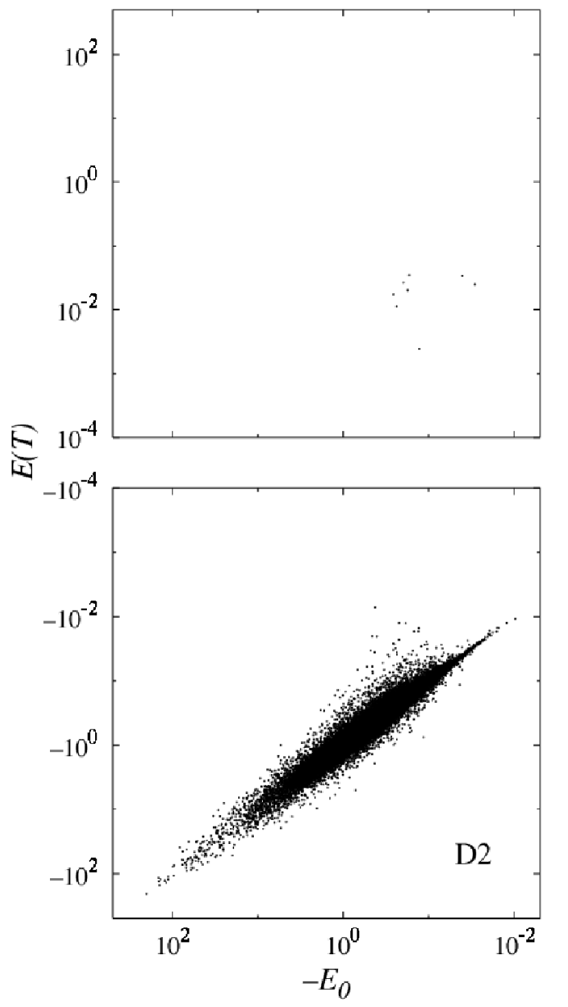
Figure 10.— Distribution of the field stars in the ($E_{0},E(T)$) planes for runs A4 and D2. $E_{0}$ is the initial specific energy and $E(T)$ is that at the time $T=1000$. Top and bottom figure shows the distribution having a positive and a negative energy, respectively.

Figures 10 show the initial and final binding energies of particles for runs A4 and D2. Here, we can see the scatter is much larger for run A4.

3.3. Evolution of eccentricity

Figure 11.— Evolution of the eccentricity of the IMBH for runs Ax.

Figure 11 shows the time evolution of the IMBH-SMBH binary eccentricity defined as

$$e=\sqrt{1-\frac{L^{2}}{(M_{S}+M_{I})a}}~{},$$ (19)

where $L$ is the angular momentum of the binary.

From these results, it is not clear if there is any systematic change in $e$ or whether or not the evolution depends on $N$. The fluctuation in $e$ is bigger for small-$N$ calculation (A1 and A2 compared to A3 or A4). On the other hand, in run A4 $e$ seems to show systematic increase after $T=600$. As we can see from figure 5, it may be related to the slowing down of the evolution of the semi-major axis, which is caused by the loss-cone depletion.

In the next section, we will investigate this evolution of the IMBH orbit after the depletion of the loss cone.

4. The evolution of IMBH orbit after the loss-cone depletion

In the previous section, we have seen that the IMBH sink toward the SMBH through dynamical friction, and its orbital evolution slows down when the IMBH reaches the radius total stellar mass inside which is comparable to the IMBH mass. In other words, it occurs after the IMBH ejected out the neighboring stars. In this section, we analyze the evolution of the IMBH orbit after it kicked out the neighboring stars. In order to do so, we performed another set of simulations (run Bx), in which we placed the IMBH initially at the distance 1/10 of that in runs Ax. Also, the stellar distribution is cut off at smaller radius, to reduce the total number of particles. We performed runs B1 through B4. The mass of the field stars in run B1 is the same as that in A4. In B4, the mass ratio between the IMBH and field stars is $10^{3}$, and therefore the mass of field stars is around the solar mass. Two-body effects in run B4 is not larger than what would occur in real galaxies.

4.1. Evolution of the semi-major axis

Figure 12.— Evolution of the semi-major axis of the IMBH. Dotted, dash-dotted, dashed, and solid curves are the results of models B1-4. Thin curve shows the theoretical curve calculated using equation (16).

Figure 12 shows the evolution of semi-major axis. We can see that the evolution does not depend on the mass of field stars. This result is not surprising since even for run B1 the initial relaxation time of field particles at the initial location of the IMBH is $7.3\times 10^{4}$ in the time unit and is much longer than the duration of the calculation. The slowing down is much more pronounced compared to that in runs Ax, simply because we followed the evolution of the IMBH down to smaller value of $a$. The evolution of the semi-major axis got stuck by $T=600$, when the semi-major axis reached $a\sim 0.003$.

Figure 13.— Energy error of the calculations. The curves give the results for runs Bx.

Figure 13 shows the energy error for each of Bx runs. Errors are reasonably small before $T=500$ for all runs. Quick increases in error are due to the increase in the eccentricity of the IMBH. At $T=500$, the binding energy of the IMBH is $\sim 60\%$ of the initial total binding energy of the system. Thus, relative energy error of $1\%$ corresponds to the error of the semi-major axis of $1.6\%$, which is small compared to the overall change of the semi-major axis.

Figure 14.— Lagrangian radii around SMBH. From bottom to top, the radii enclose $5\times 10^{-5},$ $10^{-4},2\times 10^{-4},5\times 10^{-4},$ $10^{-3},2\times 10^{-3},5\times 10^{-3},$ 0.01 and 0.02 of the unit mass. Thick solid lines indicate the semi-major axis of the IMBH.

Figure 14 shows the evolution of the Lagrangian radii of field particles. As the IMBH sinks toward the SMBH, field stars expand. As the evolution of the IMBH slows down, the expansion of field stars also slows down. It is clear that the expansion, or depletion of the loss cone, is the cause of the slowing down of the IMBH orbit evolution.

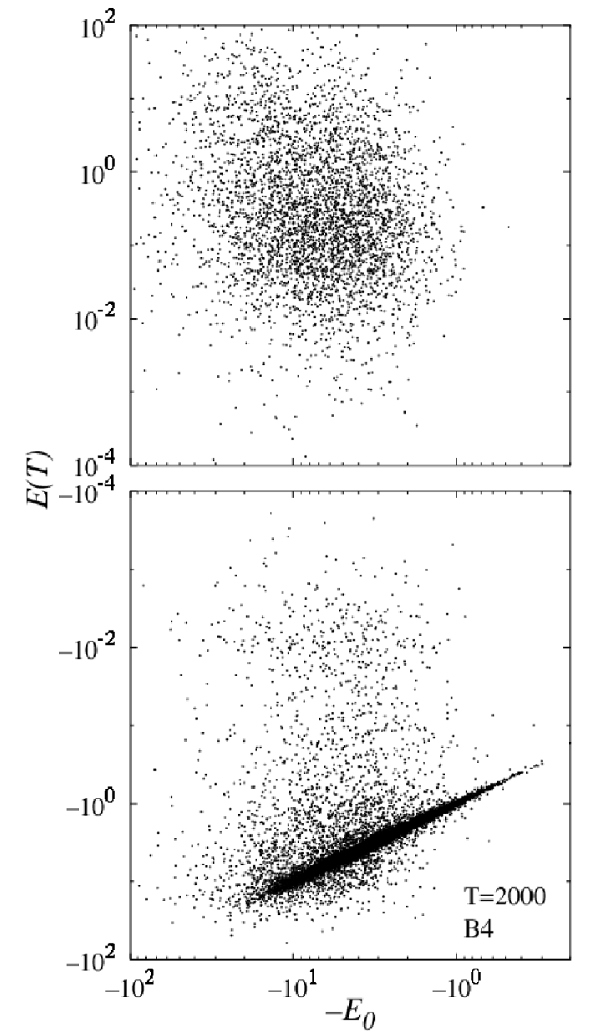
Figure 15.— Distribution of the field stars in the ($E_{0},E(T)$) plane for model B3 at $T=2000$. Top and bottom panels show the particles with positive and negative energies, respectively.

Figure 14 might give the impression that all field stars expand outward. Actually, that impression is wrong. Figure 15 shows the initial and final energies of field stars for run B3. Large fraction of field stars show very small change in the energy, and some particles get very large energy. This is of course the same as what is visible in figure 10 for run A4. Only the stars which strongly interacted with the IMBH are ejected, and other stars are essentially unaffected. The apparent expansion of outer Lagrangian radii in figure 14 is the result of the ejection of the inner part of the field stars.

4.2. Evolution of angular momentum

Figure 16.— Evolution of the eccentricity of the black hole binary. The curves give the results for runs Bx. We plot $(1-e)$ for the vertical axis.

Figure 16 shows the evolution of eccentricities for runs B1 to B4. Unlike the case of runs Ax, here it seems clear that in all runs eccentricity shows slow increase in the early phase ($T<800$), and in some runs there are phases when $e$ approaches to very close to unity. However, exactly when such phase occurs shows large run-to-run variation.

This quick increase of the eccentricity is rather surprising, since in previous studies of massive BH binaries (Makino & Funato 2004; Chatterjee et al. 2003) such increase has not been observed. However, since the configuration of the system is quite different, evolution can be very different. In the case of SMBH binary, two massive binaries have similar mass, and field stars which interact with the binary are not strongly bound to the binary. However, in our case of SMBH-IMBH binary, all field stars are strongly bound to the SMBH, and have almost Keplarian orbits. Thus, celestial-mechanical effects such as the mean-motion resonance and Kozai mechanism (kozai 1962) can play important roles. These effects, on average, work as the transport mechanism for angular momentum from rapidly-rotating objects to slowly-rotating objects. In other words, these effects tend to increase the eccentricity of the IMBH.

Figure 17.— Evolution of the normalized angular momentum of the BH binary. Dotted, dash-dotted, dashed, and solid curves give the results for $L_{x}^{*},L_{y}^{*},L_{z}^{*}$, and $L^{*}$, respectively.

Figures 17 show the normalized angular momentum of the IMBH, $L^{\ast}\equiv L/L_{0}$, where $L$ is the angular momentum calculated in Equation (19) and $L_{0}\equiv\sqrt{(M_{S}+M_{I})a}$ is the angular momentum of the circular orbit with the same semi-major axis. We can see that the slow increase of the eccentricity directly corresponds to the decrease of the total angular momentum, and the random walk of the angular momentum vector is small, especially for runs with large $N$. Apparently, only after the quick increase of the eccentricity the random walk of the angular momentum vector becomes noticeable. Thus, probably the high eccentricity state corresponds to some statistical equilibrium.

4.3. Why the eccentricity goes up?

Here we try to understand the mechanism which drives the increase of the eccentricity. We concentrate on run B4, since it has the largest number of field particles and therefore the statistical analysis of the behavior of field particles is the most reliable. In particular, as we can see in figure 17, in run B4 the orbital plane of the IMBH remains close to the xy-plane, while in other runs the random walk of the angular momentum vector is significant.

In order to understand the behavior of the IMBH, it would be useful to see with which field particles the IMBH interacted. Figure 19 shows the cumulative change of angular momentum of field particles as the function of their semi-major axis $a$. Here, the change in the angular momentum $\Delta l$ of a particle is defined as

$$\Delta l\equiv[{\bf L}(T)-{\bf L}(T+\Delta T)]\cdot\hat{\bf L}_{\rm IMBH}~{},$$ (20)

where ${\bf L}(T)$ is its angular momentum vector at time $T$, and $\hat{\bf L}_{\rm IMBH}$ is the unit vector with the direction of the angular momentum vector of the IMBH. We use $\Delta T=50$ for all values of $T$. Thus this $\Delta l$ is the angular momentum change projected to the orbital plane of the IMBH.

Figure 18.— Radial density profiles at times $T=0$, 400, 800, and $2000$ for run B4.

Figure 18 show the change of the density profiles for run B4. We can see that the central density decreases, and the inclination of the central cusp becomes flat. It is caused by the ejection of field stars by the IMBH.

Figure 19.— Cumulative change of angular momentum of field particles $\Delta l$ as a function of semi-major axis $a$ for the times $T=0$ and $800$.

The difference between the plot for $T=0$ and $T=800$ is that, even though the semi-major axis of the IMBH is much smaller at $T=800$, the field particles which exchanged the angular momentum has much wider distribution at $T=800$ than at $T=0$. For $T=0$, stars with the semi-major axis comparable to that of the IMBH dominate the change in the angular momentum, while for $T=800$, stars with $a$ comparable to that of the IMBH (0.003) have practically no contribution, and effect of stars with $a>1$ is not negligible. Of course, since the IMBH ejected most of stars with $a<0.01$, it cannot interact with them.

Figure 20.— Same as figure 19 but as a function of the periastron distance $r_{p}$ for the times $T=0$ and $800$. In the right hand panel, curves are, from top to bottom, total change, changes for particles with $a<$3.0, 1.0, and 0.3.

Figure 20 shows the same cumulative plot but as the function of the periastron distance $r_{p}$. For $T=0$, particles which go inside the IMBH orbit account for the change in the angular momentum. On the other hand, at $T=800$ particles orbit outside the IMBH orbit are responsible for the change in the angular momentum, and that tendency is more significant for field particles with small $a$.

For field stars with relatively small $a$, we can draw the following picture. The IMBH has created the hole in the distribution function, and it can interact only with stars with semi-major axis larger or comparable to its apocenter distance. In other words, the IMBH can strongly interact with other stars only when it is at the apocenter. If it loses kinetic energy at its apocenter, it becomes strongly eccentric.

Figure 21.— Comparison of run B4 and run E. As run E, we started from the $T=800$ snapshot of run B4 but we removed all stars with $a>0.3$. Left is the evolution of the eccentricity, and right is the evolution of the angular momentum of the BH binary.

Interaction with stars with large $a$ is more complex. However, here the interaction can occur at positions other than the apocenter, since field particles with large $a$ can have small $r_{p}$. Thus, the increase of the eccentricity is likely to be driven by interactions with field particles with small $a$. In order to test this hypothesis, we performed one additional run, run E, which we started from the $T=800$ snapshot of run B4 but we removed all stars with $a>0.3$. Fig 21 shows the result. The change in the eccentricity is largely similar. So we can conclude that the interactions with field stars with small $a$ (and relatively large $r_{p}$) drive the increase of the eccentricity of the IMBH.

This mechanism of the increase of the eccentricity is similar to that proposed by Fukushige et al. (1992). They argued that the dynamical friction on an eccentric binary should be most effective at the apocenter and therefore an eccentric binary should become more eccentric. For the binary SMBH of comparable masses, this mechanism turned out to be ineffective, because the change in the orbital elements of a binary is really the result of rather complex three-body interaction between two binary components and the incoming star. However, in our case of IMBH-SMBH binary, the situation is very different. Since the mass of the IMBH is much smaller than that of SMBH, field stars must come close to the IMBH to change its orbit. Thus, the IMBH does have more chance to interact with field starts at apocenter than at pericenter, and its eccentricity increases.

5. Discussion and Summary

5.1. Final fate of IMBH

We have seen that the evolution of semi-major axis of the IMBH effectively stops, when it ejected field stars in that region. We have also seen that the eccentricity of the IMBH, after the evolution of semi-major axis stopped, can reach very close to unity. From the viewpoint of the evolution of SMBH, important question is what the final fate of the IMBH is.

Figure 22.— Gravitational radiation timescale given by equation (23) for runs Bx.

Figure 22 shows the timescale of the merging through gravitational wave radiation, for runs Bx. We converted the simulation units to physical units.

The timescale of the merging through gravitational wave radiation is given by

$$t_{\rm gr} = {5\over 256}\frac{a^{4}c^{5}}{G^{3}M_{S}M_{I}(M_{S}+M_{I})}F(e)$$ (21)

with $F(e)$ is

$$F(e) = \left({1-e^{2}}\right)^{7/2}\left({1+\frac{73}{24}e^{2}+\frac{37}{96}e^{4}}\right)^{-1}$$ (22)

(Peters 1964). The timescale $t_{\rm gr}$ depends strongly on $e$, when $e$ is close to unity. In our units, $t_{\rm gr}$ is given by

$$t_{gr} \simeq 6.3\times 10^{13}F(e)$$ (23)

$$\left({a\over 0.01\rm pc}\right)^{4}\left({M_{S}\over 3\times\!10^{6}M_{\odot}}\right)^{-2}$$

$$\left({M_{I}\over 3\times\!10^{3}M_{\odot}}\right)^{-1}{\rm yr}.$$

We can see from figure 22 that the merging timescale can go down to less than $10^{6}$ yrs, and stays at that value for some time. In other words, if we take into account the effect of gravitational wave radiation, the IMBH will merge to SMBH.

5.2. Event rate for gravitational wave detection

Matsubayashi et al. (2004) estimated the event rate of the merging of IMBH-SMBH binary, assuming that all binaries eventually merge. Our present result indicates that this assumption of 100% merging is valid. They estimated the event rate to be $20\sim 70$ per year, for the detection limit of $h\approx 10^{-21}$. Here, $h$ is the dimensionless amplitude of gravitational wave. The frequency of the gravitational wave in their final merging phase is $10^{-1}$ to $10^{2}$ Hz. It is within the target range of LISA(LISA report 2000) and DECIGO(Seto et al. 2001).

Matsubayashi et al. (2004) considered two limiting cases for the growth of SMBH. In the first case, the growth is hierarchical. BHs always merge with another BH with a similar mass. In the second case, the growth is monopolistic and one BH always merge with IMBH of small mass. In the first case, large number of events has rather low amplitude, since they come from IMBH-IMBH mergings. In the second case, most events come from IMBH-SMBH merging, and therefore amplitude is bigger than that in the first case. DECIGO will be able to detect all events for both cases, while LISA would not detect the majority of events in the case of hierarchical growth. In the case of the monopolistic growth, both DECIGO and LISA will detect most of events. Thus, DECIGO event rate would be around 50, while LISA event rate would be 5-50, depending on the growth mode.

5.3. Summary

In this paper, we studied the orbital evolution of the IMBH after its parent cluster is completely disrupted. Our main findings are summarized as follows.

Initially, the IMBH sink toward the SMBH through dynamical friction. However, the evolution of the semi-major axis stops when the IMBH approaches to the radius at which the initial stellar mass is comparable to the IMBH mass. For our galaxy, it corresponds to around 0.01 pc. If the IMBH remains in a circular orbit, the merging timescale by gravitational wave radiation would be $6.3\times 10^{13}$ yrs.

However, in this region the eccentricity of the IMBH approaches to unity, and therefore we expect the IMBH to quickly merge with the SMBH. This increase is due to interactions with field stars with periastron larger than the semi-major axis of the IMBH. The fact that many of the stars very close to the galactic center have large eccentricities is probably explained by the same mechanism. For example, S2 has $e\sim 0.87$ and $a\sim 0.119^{\prime\prime}(\simeq 4\times 10^{-3}pc)$(Schodel et al. 2003). The distribution of eccentricities of known stars very close to SgrA* is not consistent with being isotropic.

References

- Alcubierre et al. (2001) Alcubierre, M., Bernger, W., Bruegmann, B., Lanfermann, G., Nerger, L., Seidel, E., and Takahashi, R., 2001, Phys. Rev. Lett., 87, 271103
- Bahcall & Wolf (1976) Bahcall, J. N., & Wolf. R. A., 1976, ApJ, 209, 214
- Binney & Tremaine (1987) Binney, J. J., & Tremaine, S., 1987, Galactic Dynamics (Princeton University Princeton Press)
- Begleman, Blandford, & Rees (1980) Begelman, M. C., Blandford, R. D., & Rees, M. J., 1980, Nature, 287, 307
- Berczik et al. (2005) Berczik,P., Merritt, D., & Spurzem, R., 2005, ApJ633, 680
- Ebisuzaki et al. (2001) Ebisuzaki, T., Makino, J., Tsuru, T.G., Funato, Y, Zwart, S.P., Hut, P., McMillan, S., Matsushita, S., Matsumoto, H., & Kawabe, R. 2001, ApJ, 562, L19
- Fukushige et al. (2005) Fukushige, T., Makino, J., & Kawai, A., 2005, PASJ, in press, astro-ph/0504407
- Fukushige et al. (1992) Fukushige, T., Ebisuzaki, & T., Makino, J., 1992, PASJ, 44, 281
- kozai (1962) Kozai, Y., 1962, AJ, 67, 591
- Chatterjee et al. (2003) Chatterjee, P., Hernquist, L., & Loeb, A., 2003, ApJ, 592, 32
- Guesten et al. (1987) Guesten, R., Genzel, R., Wright, M. C., Jaffe, D. T., Stuzki, J., & Harris, A. I., 1987, ApJ, 318, 124
- Genzel et al. (1996) Genzel, R., Thatte, N., Krabbe, A., Kroker, H., & Tacconi-Garman, L. E., 1996, ApJ, 472, 153
- Genzel et al. (1997) Genzel, R., Eckart, A., Ott, T., & Eisenhauer, F., 1997, MNRAS, 291, 219
- Genzel et al. (2000) Genzel, R., Pichon, C., Eckart, A., Gerhard, O. E., & Ott, T., 2000, MNRAS, 317, 348
- Hashimoto et al. (2003) Hashimoto, Y., Funato, Y., & Makino, J., 2003, ApJ, 582, 196
- Kawakatu (2002) Kawakatu, N., & Umemura, M., 2002, MNRAS, 329, 572
- LISA report (2000) LISA Laser Interferometer Space Antenna: A Cornerstone Mission for the Observation of Gravitational Waves, System & Technology Study Report, ESA-SCI (2000) 11
- Makino & Aarseth (1992) Makino, J., & Aarseth, S. J., 1992, PASJ, 44, 141
- Makino (1997) Makino, J., 1997., ApJ, 478, 58
- Makino et al. (2003) Makino, J., Fukushige, T., Koga, M., & Namura, K., 2003, PASJ, 55, 1163
- Makino & Funato (2004) Makino, J., & Funato, Y. 2004, ApJ, 602, 93