A Galactic Origin for the Local Ionized X-ray Absorbers

Abstract

Recent Chandra and XMM observations of distant quasars have shown strong local ($z\sim 0$) X-ray absorption lines from highly ionized gas, primarily He-like oxygen. The nature of these X-ray absorbers, i.e., whether they are part of the hot gas associated with the Milky Way or part of the intragroup medium in the Local Group, remains a puzzle due to the uncertainties in the distance. We present in this paper a survey of 20 AGNs with Chandra and XMM archival data. About 40% of the targets show local O VII He $\alpha$ absorption with column densities around $10^{16}\ \rm cm^{-2}$; in particular, O VII absorption is present in all the high quality spectra. We estimate that the sky covering fraction of this O VII-absorbing gas is at least 63%, at 90% confidence, and likely to be unity given enough high-quality spectra. Based on (1) the expected number of absorbers along sight lines toward distant AGNs, (2) joint analysis with X-ray emission measurements, and (3) mass estimation, we argue that the observed X-ray absorbers are part of the hot gas associated with our Galaxy. Future observations will significantly improve our understanding of the covering fraction and provide robust test of this result.

1. Introduction

Recently, a number of Chandra and XMM-Newton observations of quasars have shown local ($z\approx 0$) X-ray absorption lines (Kaspi et al., 2002; Nicastro et al., 2002; Fang et al., 2002; Rasmussen, Kahn, & Paerels, 2003; Fang, Sembach, & Canizares, 2003; Cagnoni et al., 2004; McKernan et al., 2004; Williams et al., 2005). These background quasars are among the brightest extragalactic X-ray sources in the sky and some of them were used as calibration targets. The typical high ionic column densities of these X-ray absorbers ($\sim 10^{16}$ $\rm cm^{-2}\$) imply the existence of large amounts of hot gas with temperatures around $10^{6}$ K. Recent ultraviolet observations of the local high velocity O VI absorbers also reveal such hot gas but at lower temperatures (see. e.g., Sembach et al., 2003; Nicastro et al., 2003). Given the spectral resolution of Chandra and XMM-Newton, it is still unclear where this hot gas is located: in the interstellar medium, in the Galactic halo, or in the Local Group as the intragroup medium.

In sharp contrast, so far only four targets were reported showing intervening absorption systems ($z>0$), all with low ion column densities. Fang et al. (2005) confirmed their first detection (Fang et al., 2002) of an absorption system at $z\sim 0.055$, along the sight line towards PKS 2155-304. They found the observed O VIII column density is $\sim 4\times 10^{15}$ $\rm cm^{-2}\$, and set a 3$\sigma$ upper limit on the O VII column density of $\sim 10^{15}$ $\rm cm^{-2}\$at the same redshift. Nicastro et al. (2005) reported the detection of two absorption systems along the sight line towards Mkn 421, but both systems showed O VII absorption lines with column densities less than $10^{15}$ $\rm cm^{-2}\$. Mathur, Weinberg, & Chen (2002) reported a number of X-ray absorption systems towards H 1821+643 at 2 - 3 $\sigma$ level, and McKernan et al. (2003) reported the detection of an O VIII absorption line along the sight line towards 3C 120.

To understand the difference between the local and intervening absorption systems, we conduct a survey of a number of extragalactic targets observed with Chandra and XMM-Newton to search for local X-ray absorption lines. In this paper, we report the result of this survey. We find that a model in which local X-ray absorbers are associated with the Milky Way can explain our survey results better than a model in which they are associated with the intragroup medium in the Local Group. Recently, McKernan et al. (2004) conducted a systematic survey of 15 nearby AGNs to investigate the hot X-ray absorbing gas in the vicinity of the Galaxy. While their work mainly focuses on associating individual line of sight with known local structures, our work is different in that we study the generic properties of this hot gas.

2. Sample Selection and Data Reduction

All the background sources are selected from the Chandra and XMM-Newton data archives. We focus on instruments that can provide both high spectral resolution and moderate collecting area in the soft X-ray band, and this results in four different instrument combinations: (1) RGS, the Reflection Grating Spectrometer; (2) LETG (the Low Energy Transmission Grating) + HRC (the High Resolution Camera); (3) LETG + ACIS (the Advanced CCD Imaging Spectrometer); and (4) HETG (the High Energy Transmission Grating) + ACIS. The first one (RGS) is on board XMM-Newton and the last three are instruments on board Chandra. The instrumental resolving power is typically characterized by the line response function (LRF), the underlying probability distribution of a monochromatic source. HETG-ACIS has the highest resolving power: the LRF of the Medium Energy Grating (MEG) has a full width at half maximum (FWHM) of $\Delta\lambda\sim 0.02$ Å  around 20 Å.  The other three combinations have a roughly constant resolution of $\Delta\lambda\approx 0.05\,\AA$ across the relevant wavelength range. In some cases, a target has been observed with several different instrument configurations, and we select those that give the highest number of continuum counts.

So far, nearly all the sources with local X-ray absorption lines show the detection of O VII with high confidence, so in this paper we concentrate on the O VII He$\alpha$ resonance line with a rest wavelength of 21.6 Å . To ensure the significance of the absorption line, we select targets that have a strong continuum between 21 and 23 Å . Specifically, we bin the spectrum to roughly half of the LRF FWHM and select targets which have at least 10 counts per bin around 21.6 Å . In this way, we can ensure a signal-to-noise ratio (SNR) of at least 4 within the LRF. We test with other binning size and find essentially similar results.

Table 1: O VII He$\alpha$ Absorption Line
Target	Redshift	Inst.a	Cont.b	${\rm EW}$c	$S/N$d	${\rm EW_{\rm th}}$e	Notef
MS 0737+7441	0.315	1	10	…	…	24
NGC 3227	0.0039	2	12	…	…	22
NGC 4258	0.0015	2	17	…	…	18
Ton S180	0.0620	3	17	…	…	18
MCG 6-30-15	0.0078	4	23	$18_{-8}^{+10}$	4.1	13
NGC 7469	0.0163	1	32	…	…	13
NGC 4593	0.009	2	34	$17\pm 9$	3.3	13	1
Mkn 766	0.0129	1	35	…	…	13
H 1426+428	0.129	1	35	…	…	13
Ton 1388	0.1765	2	37	…	…	12
PKS 0558-504	0.137	1	40	…	…	12
Mkn 501	0.0337	1	40	…	…	12
NGC 3783	0.0097	4	47	$36^{+27}_{-11}$	6.3	9	2
1H 1219+301	0.182	1	50	…	…	11
H 1821+643	0.297	3	59	…	…	10
3C 273	0.1583	3	70	$28_{-6}^{+12}$	6.4	9	3
NGC 5548	0.0172	1	140	$10\pm 5$	3.3	6	4
NGC 4051	0.0023	1	144	$17_{-6}^{+2}$	5.5	6	5
PKS 2155-304	0.156	3	350	$15_{-3}^{+4}$	7.1	4	6
Mkn 421	0.03	1	1500	$9.4\pm 1.1$	8.8	2	7

a. Instrument: 1 — RGS; 2 — LETG-HRC; 3 — LETG-ACIS; 4 — HETG-ACIS.

b. Continuum level, in units of counts per bin. The bin size is 0.02 Å for HETG and 0.025 Å  for others.

c. Equivalent width of detected O VII He$\alpha$ absorption line, in units of mÅ.

d. Signal-to-noise ratio.

e: the minimum equivalent width that can be detected at 3$\sigma$.

f. References on previously reported detections: 1 – Steenbrugge et al. (2003a); 2 – Kaspi et al. (2002); 3 – Fang, Sembach, & Canizares (2003); 4 – Steenbrugge et al. (2003b); 5 – Pounds et al. (2004); 6 – Fang et al. (2005); 7 – Williams et al. (2005)

Both Chandra and XMM-Newton data are analyzed using standard software, i.e., CIAO 3.1 and SAS 6.0. We refer readers to Fang et al. (2005) for detailed data analysis procedures. The local O VII He$\alpha$ absorption lines from 8 of our 20 targets targets have been reported previously by other papers; however, to ensure consistency in our data analysis, we re-analyze all the data sets and fit the absorption lines to obtain the equivalent width (EW) independently (see column 5 of Table 1), and we refer the readers to the references we list in the column 7 of Table 1 for spectra of detected O VII lines. Due to the complex nature of the sources in our sample and possible residual calibration effects, instead of fitting the continuum with a physically meaningful model such as an absorbed power law, we fit the continuum between 21 and 23 Å  with a polynomial of an order between 3 to 5, to effectively remove residual feature on scales $\gtrsim 0.4$ Å. The residual is then fitted with a Gaussian at $\sim 21.6$ Å, using ISIS (Interactive Spectral Interpretation System, see Houck & Denicola, 2000) . While in all cases we confirm the detections (and non-detections) that were reported by the original authors, in some cases our measured EWs are smaller than those originally reported. For example, we obtain an EW of $17\pm 9$ mÅ for NGC 4593, while Steenbrugge et al. (2003a) report a much larger value, $45\pm 31$ mÅ. A careful reexamination of both data analysis procedures indicates that the main discrepancy comes from the determination of the continuum level (Steenbrugge, private communication.) Nevertheless, our method is more stringent and the measured EWs can be taken as conservative lower limits.

Figure 1.— An all-sky Hammer-Aitoff projection of the 20 sight lines in our entire sample.

Some of the sources in our sample are known to have intrinsic warm absorbers. One may worry that the absorption lines detected at 21.6 Å could be associated with the intrinsic warm absorbers, particularly in the case of NGC 3783 where Ca XVI may account for part of the absorption (Krongold et al., 2003). However, this does not have a significant impact on our conclusions. Our case-by-case study of all the warm-absorbers in our sample indicates that O VII and Ca XVI are the only possible sources of confusion. O VII is unlikely because except in NGC 4051, none of the known warm-absorbers show the outflow velocities that can compensate their redshifts. For Ca XVI, our study indicates that O VIII always co-exists with Ca XVI but with at least $\sim 300$ times higher column density, so a non-detection of O VIII or a detection of O VIII with column density lower than $\sim 10^{18}$ $\rm cm^{-2}\$would simply rule out the presence of Ca XVI. By looking at each case, we find that Ca XVI can have a contribution only for NGC 3783 and MCG–6-30-15. While Ca XVI can contribute at most part of the 21.6 Å line in NGC 3783, the contribution to MCG–6-30-15 is unknown yet. To be conservative, we therefore consider a subsample that excludes NGC 3783 and MCG–6-30-15.

The sight line to 3C 273 extends into the Galactic halo through the edges of Radio Loops I and IV, which have been attributed to supernova remnants (see, e.g., Egger & Aschenbach, 1995). Fang, Sembach, & Canizares (2003) estimated that the contribution to the O VII column density from the supernova remnants accounts for at most 50% of the observed equivalent length.

If the absorption line is unsaturated, the equivalent width of the O VII He$\alpha$ absorption line can be converted to a column density by (Spitzer, 1978)

$$N(\rm OVII)=7\times 10^{15}\left(\frac{{\rm EW}}{20\rm\,mA}\right)\,cm^{-2}.$$ (1)

However, saturation could be an important issue, as revealed by high-order transition O VII lines discovered in the Mkn 421 spectrum (Williams et al., 2005), the highest quality spectrum in our sample. In that case, the column density of O VII, determined by high-order transition lines is $\sim 1.6\times 10^{16}$ $\rm cm^{-2}\$, more than five times higher than that estimated from Eq.(1). With this consideration, column densities converted from Eq.( 1) can serve as conservative lower limits, and we adopt $10^{16}\rm\,cm^{-2}$ as a fiducial value in the following discussion for simplicity.

In Figure 2 we show an all-sky projection of the entire sample in our survey. The green dots show the positions of those targets with detections, and the red dots show the positions of those without detections.

We wish to estimate the fraction of the sky covered by gas with an O VII equivalent width of at least EW, $C({\rm EW})$. The difficulty we face is that we have a limited sample size, and not all sources in our sample have enough counts to permit detection of an absorption line of equivalent width EW. For each source, we define the threshold equivalent width, ${\rm EW_{\rm th}}$, which is the minimum equivalent width that can be detected at 3$\sigma$:

$${\rm EW_{\rm th}}=3\left(\frac{\lambda}{F_{\lambda}ATR}\right)^{1/2},$$ (2)

where $\lambda$ is wavelength, $F_{\lambda}$ is the photon flux, $A$ is the area of the detector, $T$ is the observation time, and $R\equiv\lambda/\Delta\lambda$ is the resolving power where $\Delta\lambda$ is the width of a resolution element. ${\rm EW_{\rm th}}$ therefore depends on both the detector and the source; as more data are gathered for a given source, its value of ${\rm EW_{\rm th}}$ will decrease. Table 1 includes values of ${\rm EW_{\rm th}}$ for each source in our sample.

To estimate $C({\rm EW})$, we consider all the sources with ${\rm EW_{\rm th}}<{\rm EW}$, since only these sources have enough counts to ensure detection of an absorption system with an equivalent width ${\rm EW}$. Let ${\cal N}({\rm EW})$ be the number of these sources, and let ${\cal N}_{\rm det}({\rm EW})$ be the number of sources in this sample with detectable OVII absorption (by definition, such sources must have ${\rm EW}\geq{\rm EW_{\rm th}}$). The detection fraction is then

$$F({\rm EW})\equiv\frac{{\cal N}_{\rm det}({\rm EW})}{{\cal N}({\rm EW})},$$ (3)

and in the limit of large ${\cal N}_{\rm det}({\rm EW})$ it will approach $C({\rm EW})$. Figure 2 shows the detection fraction as a function of the minimum detectable equivalent width, and the error bars are the standard 1$\sigma$ errors for a binomial distribution. We show the error bars for the entire sample only for demonstration purposes. The detection fraction starts at $\sim$10% for the entire sample and $\sim$ 5% for the subsample, corresponding to lines with ${\rm EW}\gtrsim 20$ mÅ, and then gradually increases to 100% with increasing continuum level or decreasing EW threshold. The most striking feature is that the detection fraction approaches 100% as the sensitivity approaches ${\rm EW}\sim 10$ mÅ, which occurs at a continuum level of $\sim 60$ counts per bin. While it is tempting to infer that the detection fraction would be 100% if our sample had enough sensitivity, we must be cautious: given the detections of O VII absorption lines in the five highest-quality data sets, we can conclude only that we have 90% confidence that the sky detection fraction is at least $(1-0.9)^{1/5}$, or 63%.

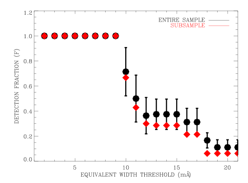
Figure 2.— The covering factor as a function of the equivalent width threshold. Dark line shows the entire sample and red line shows the subsample, and the error bars are the standard 1$\sigma$ error for binomial distribution.

3. Where is the X-ray absorbing gas?

While both Chandra and XMM-Newton have unprecedented resolving power, the highest resolution we can achieve (HETG-ACIS, in this case) is about $300$ $\rm km\ s^{-1}$. Based on the Hubble flow and adopting a Hubble constant of $H_{0}=70\rm\,km\,s^{-1}Mpc^{-1}$, this corresponds to a distance of $\sim 4$ Mpc at $z\sim 0$, which makes it impossible to distinguish between a Milky Way-origin (with a halo radius of $\lesssim 0.1$ Mpc) and a Local Group-origin (with a radius of $\sim 1$ Mpc) for the X-ray absorbers. Nevertheless, with such a large sample size, we can begin to understand the properties of these absorbers, i.e., their size, density, temperature, spatial distribution, etc. In the previous section, we estimate the sky detection fraction $F$ of this hot gas. The detection fraction $F$ can be taken as an estimate of sky covering fraction, defined as $C\sim F$. Our estimation then indicates that the sky cover fraction is at least higher than 63%, and is likely close to unity. In the following, based on this estimation we (1) calculate the expected number of absorbers along lines-of-sight toward distant AGNs, (2) make joint analysis with X-ray emission measurements, and (3) estimate the total baryonic mass. Our calculation indicates that the observed X-ray absorbers are associated with our Galaxy.

3.1. Expected Number of Absorbers along LOSs toward Distant AGNs

Given the high quality of spectra in our sample, any absorbers distributed between us and background AGNs with similar column densities, i.e., $\rm N(O{\rm VII})\sim 10^{16}$ $\rm cm^{-2}\$, would be detected with high confidence. Now let us estimate the expected number of intervening absorbers with a similar O VII column density in our sample.

A key assumption in our model is that the X-ray absorbers detected at $z\sim 0$ are not unique, i.e., an observer located in another galaxy similar to the Milky Way should be able to see similar X-ray absorption. The next step is to convert the covering fraction that we presented in the previous section to the detectability of these absorbers around systems similar to the Milky Way or the Local Group, along the sight lines towards background AGNs.

We assume that the X-ray absorbers are uniformly distributed within the halo (of a galaxy or a group of galaxies) that has a radius $R$. Let $C$ be the sky covering factor as observed from the center of the distribution of absorbers, which can be obtained from observation. If we view the absorbers in a different group of galaxies, the observed covering factor would be $\frac{4}{3}C$ (see, e.g., Tumlinson & Fang, 2005). Given the spatial density of the absorbers within the halo, we can then calculate the expected number of absorbers along the total line of sight towards all the background sources in our sample. If the spatial density of halos with radius $R$ is $\phi_{0}$, the expected number is then

$${\cal N}_{\rm obs}=\int_{0}^{\ell_{\rm tot}}\frac{4C}{3}\phi_{0}\sigma_{0}d\ell,$$ (4)

where $\sigma_{0}=\pi R^{2}$ is the cross section and $\ell_{\rm tot}$ is the cumulative distance along the sight lines to all the targets in the sample.

In reality, both the covering fraction and the available pathlength, and so $N_{obs}$, depend on the detection threshold ${\rm EW_{\rm th}}$. Taking the covering fraction from Eq. (3), we can calculate $N_{obs}$ from Eq. (4), as a function of ${\rm EW_{\rm th}}$ (Figure 3). Let us consider two scenarios, in which the absorbers can be associated either with Milky Way-type halos or with Local Group-type halos. For the Milky Way-type halo, $R\lesssim 100$ kpc, and the spatial density of halos is just the spatial density of $L_{\star}$ galaxies, i.e., $\phi_{0}\sim 0.004\rm\,Mpc^{-3}$ (Blanton et al., 2003). On the other hand, if the observed local absorbers are associated with the Local Group, $R$ would be $\sim 1$ Mpc. An integral over the Press-Schechter mass function (Press & Schechter, 1974) from $10^{12}$ to $10^{13}\rm\,M_{\odot}$ gives a halo spatial density of $\phi_{0}\approx 0.0007\rm\,Mpc^{-3}$. In figure 3, Local group case and the Milky Way case are represented by solid and dashed lines, respectively. Dark lines are for the entire sample, and red lines are for the subsample. Given the fact that none of the targets in the sample show any intervening absorption O VII with column densities even close to $5\times 10^{15}$ $\rm cm^{-2}\$, clearly the observations are consistent with the association of the local X-ray absorbers with Milky Way-type halos, but inconsistent with a Local Group association. In the Local Group case, for the entire sample the maximum expected number of absorbers is $\sim 9.4$ if we take a threshold of $\sim 9$ mÅ. The Poisson probability of detecting zero if the expectation is 9.4 is just $\exp(-9.4)\sim 0.008\%$, at above Gaussian $3.7\sigma$ level. If we take the subsample, the expected number decrease to $\sim 9.1$, and the probability increases to $\sim 0.01\%$, roughly corresponding to a Gaussian $3.7\sigma$ level.

Figure 3.— The expected number of absorbers as a function of the equivalent width threshold. Local group case and the Milky Way case are represented by solid and dashed lines, respectively. Dark lines are for the entire sample, and red lines are for the subsample.

3.2. Mass Estimation

We can also estimate the total baryon mass in these X-ray absorbers. Let $n_{\rm H}$ be the hydrogen density in an absorber and let $f_{a}$ be the volume filling factor of the absorbers in the halo. Let $N_{\rm H}$ be the typical hydrogen column density along lines of sight in which X-ray absorption is seen. Averaged over the sky, the average column density is $CN_{\rm H}=f_{a}n_{\rm H}R$, so that the baryonic mass of the absorbers is $M_{b}=(4\pi R^{3}/3)f_{a}\mu_{\rm H}n_{\rm H}=(4\pi R^{2}/3)C\mu_{\rm H}N_{\rm H}$, where $\mu_{\rm H}=2.3\times 10^{-24}$ g is the mass per H. Let $f$(O VII) be the ionization fraction of O VII and $Z/Z_{\odot}$ be the abundance of oxygen relative to the solar abundance (taken as $4.6\times 10^{-4}$ — Asplund et al., 2004). We then have

$$M_{b}=\frac{4\pi}{3}CR^{2}\mu_{\rm H}\left[\frac{N({\rm O\ VII})}{4.6\times 10^{-4}f({\rm O\ VII})Z/Z_{\odot}}\right]\;,$$ (5)

where the factor in brackets equals $N_{\rm H}$. If the absorbers were distributed throughout the Local Group so that $R\sim 1$ Mpc, their total mass would be $M_{b}\simeq 1\times 10^{12}C/[(Z/Z_{\odot})f$(O VII)] $M_{\odot}$. Since the dynamical mass of the Local Group is $\sim 2\times 10^{12}\ M_{\odot}$ (see, e.g., Courteau & van den Bergh, 1999), the total baryon mass in the Local Group is $\sim 3\times 10^{11}\ M_{\odot}$ for a baryon fraction of $\sim$ 15%. This means the covering fraction at most can be 30% for solar metallicity. Since figure 2 clearly indicates that the covering fraction can be much higher (and probably be as high as $\sim 100\%$) given enough instrumental sensitivity, we conclude that a Local Group origin for these X-ray absorbers is unlikely because their estimated total mass would exceed the baryon mass of the Local Group. Our conclusion is consistent with that of Collins et al. (2005) On the other hand, if we associate these absorbers with our Galaxy, then the radius decreases by a factor of 10-100 and the total mass is substantially reduced.

3.3. Joint Analysis with X-ray Emission Measurements

Having presented evidence associating the $z=0$ X-ray absorbers with the hot gas within the Milky Way, we can further constrain the properties of the X-ray absorbers by assuming that the same absorbers are also responsible for at least some of the hot halo foreground observed in X-ray emission. The soft X-ray background is believed to be produced by three components: the Local Hot Bubble (LHB), the extragalactic background (mainly from point sources), and a halo component. By analyzing Rosat All Sky Survey (RASS) data, Kuntz & Snowden (2000) concluded that the halo emission actually consists of two components, a hard component with $\log T_{H}=6.46$ and a soft component with $\log T_{S}=6.06$. Because the hard component is too hot to produce a substantial amount of O VII in collisional ionization equilibrium, we assume that most of the observed O VII resides in the soft component.

Let ${\rm EM}_{\rm obs}$ be the observed emission measure. Since ${\rm EM}_{\rm obs}$ is based on solar abundances and is averaged over the sky, it is related to the actual emission measure, EM, along a line of sight through an absorber by ${\rm EM}_{\rm obs}\simeq(Z/Z_{\odot})C\;{\rm EM}=(Z/Z_{\odot})Cn_{e}n_{p}L_{\rm pc}$, where $n_{e}\simeq 1.2n_{p}$ and $n_{e}$ and $n_{p}$ are the electron and proton densities. $L_{\rm pc}$ is the average pathlength through an absorber in pc. Kuntz & Snowden (2000) found an emission measure of ${\rm EM}_{\rm obs}=4.7\times 10^{-3}\rm\,cm^{-6}\,pc$ for the soft component. From the absorption measurement, we have $N({\rm O\;VII})=4.6\times 10^{-4}(Z/Z_{\odot})f_{OVII}n_{\rm H}L\sim 10^{16}$ $\rm cm^{-2}\$. Since $f_{OVII}\simeq 1$ at $\log T_{S}=6.06$, we have $n_{\rm H}\simeq 5.6\times 10^{-4}/C\rm\;cm^{-3}$ (independent of metallicity), and $L\simeq 13C(Z_{\odot}/Z)$ kpc. This also provides independent evidence that these X-ray absorbers should be associated with our Milky Way instead of the intragroup medium in the Local Group.

4. Discussion

Rasmussen, Kahn, & Paerels (2003) argued that based on a combination of O VII emission line and absorption line measurement, the scale length of the O VII absorber should be at least $140/(Z/Z_{\odot}/0.3)$ kpc. However, their argument depended crucially on the temperature of the emitter/absorber. A shift in temperature by 0.1 to 0.2 in log space will change the scale length by a factor of 10. They determined the temperature should be between $2-5\times 10^{6}$ K, based on the O VIII and O VII line ratio. A recent work, based on much higher quality Chandra data on Mkn 421 (Williams et al., 2005), indicated that just from Chandra measurement of the O VIII and O VII line ratio, the temperature of the Mkn 421 local absorber must be lower than $1.6\times 10^{6}$ K. Such a temperature brings the scale length down to the Galactic scale.

We estimate this X-ray absorbing gas has a density of a few $\times 10^{-4}\rm\;cm^{-3}$ with temperature around $10^{6}$ K. Our estimations are consistent with values predicted from other models such as the dynamics of the Magellanic Stream (Moore & Davis, 1994). Heckman et al. (2002) suggested, based on observations of O VI absorption in the disk and halo of the Milky Way and in the intergalactic medium, that these absorption systems belong to radiative cooling flow of hot gas. Their predicted O VII column density is consistent with what we find in this paper. A key question then is: how to keep this gas hot without cooling? For gas with such a high density, the cooling time will be less than the Hubble time. In collisional ionization equilibrium, the typical cooling time scale is

$$t_{c}\sim 0.25\;\frac{T_{6}}{n_{-3}\Lambda_{-22}}~{}~{}{\rm Gyr},$$ (6)

with $n_{-3}=n_{H}/(10^{-3}\,\rm cm^{-3})$ and $T_{6}=T/(10^{6}\,\rm K)$. Here, $n_{\rm H}^{2}\Lambda_{-22}$ is the radiative cooling rate in units of $\rm 10^{-22}\,erg\,cm^{-3}s^{-1}$. Under the assumption that the cooling rate at $T_{6}\sim 1$ scales as the Fe abundance, the cooling rate of Sutherland & Dopita (1993) is $\Lambda_{-22}\simeq 0.85(Z/Z_{\odot})T_{6}^{-0.8}$, where the solar abundances are taken from Asplund et al. (2004). For the density and temperature we have estimated for the absorbers, the cooling time is much less than the Hubble time, unless the metallicity is extremely low ($Z/Z_{\odot}\lesssim 0.025$).

To keep this relatively dense gas ($n_{e}\lesssim 10^{-3}$ $\rm cm^{-3}$) at temperatures around $10^{6}$ K without cooling down over a Hubble time scale, some sort of heating mechanism must play an important role. Supernova heating is a potential candidate. The cooling rate, according to the calculations above, would be

$${\cal L}=n_{\rm H}\Lambda(M_{b}/\mu_{\rm H})\approx 4.2\times 10^{41}(R/100\;{\rm kpc})^{2}~{}~{}~{}\rm erg\,s^{-1},$$ (7)

for $T_{6}\simeq 1$; note that the dependence on $C$, $f$(O VII), and $Z/Z_{\odot}$ has canceled out. Assuming that the supernova rate is about 0.02 yr^-1 in our Galaxy (see, e.g., Dragicevich et al., 1999), and that the energy output of each supernova explosion is about $10^{51}\rm\,erg$, the heating rate would be about $6.3\times 10^{41}\,\rm erg\,s^{-1}$. For $R\ll 100$ kpc, which is consistent with our estimate for $L$, only a small fraction of the supernova energy is needed to maintain the temperature of the absorbers at $T\sim 10^{6}$ K.

In this paper, we find that the sky covering fraction of this hot, O VII-absorbing gas is at least 63%, at 90% confidence. This is based on the detections of O VII absorption lines at $>3\sigma$ level in the spectra of the top five high quality spectra. While we cannot obtain the exact location of this hot gas within our Galaxy, joint analysis with the X-ray background data indicates the scale height of this hot gas should be $\simeq 13C(Z_{\odot}/Z)$ kpc. Finally we conclude that, based on three independent estimations, the X-ray absorbing gas detected locally are part of the hot gas in our Galaxy. Future observations will provide robust test of this result.

Acknowledgments: We thank Julia Lee for help with MCG 6-30-15 data and Rik Williams for help with Mkn 421 data. We also thank the anonymous referee for valuable suggestions. TF was supported by the NASA through Chandra Postdoctoral Fellowship Award Number PF3-40030 issued by the Chandra X-ray Observatory Center, which is operated by the Smithsonian Astrophysical Observatory for and on behalf of the NASA under contract NAS 8-39073. The research of CFM was supported in part by NSF grant AST00-98365 and by the support of the Miller Foundation for Basic Research. MGW was supported in part by a NASA Long Term Space Astrophysics Grant NAG 5-9271.

References

- Asplund et al. (2004) Asplund, M., Grevesse, N., Sauval, A. J., Allende Prieto, C., & Kiselman, D. 2004, A&A, 417, 751
- Blanton et al. (2003) Blanton, M. R., et al. 2003, ApJ, 592, 819
- Cagnoni et al. (2004) Cagnoni, I., Nicastro, F., Maraschi, L., Treves, A., & Tavecchio, F. 2004, ApJ, 603, 449
- Collins et al. (2005) Collins, J. A., Shull, J. M., & Giroux, M. L. 2005, ApJ, accepted, (astro-ph/0501061)
- Courteau & van den Bergh (1999) Courteau, S., & van den Bergh, S. 1999, AJ, 118, 337
- Dragicevich et al. (1999) Dragicevich, P. M., Blair, D. G., & Burman, R. R. 1999, MNRAS, 302, 693
- Egger & Aschenbach (1995) Egger, R. J., & Aschenbach, B. 1995, A&A, 294, L25
- Fang et al. (2002) Fang, T., Marshall, H. L., Lee, J. C., Davis, D. S., & Canizares, C. R. 2002, ApJ, 572, L127
- Fang, Sembach, & Canizares (2003) Fang, T., Sembach, K. R., & Canizares, C. R. 2003, ApJ, 586, L49
- Fang et al. (2005) Fang, T., Canizares, C. R., & Marshall, H. 2005, ApJ, submitted
- Fang et al. (2005) Fang, T., et al. 2005, ApJ, in preparation
- Heckman et al. (2002) Heckman, T. M., Norman, C. A., Strickland, D. K., & Sembach, K. R. 2002, ApJ, 577, 691
- Houck & Denicola (2000) Houck, J. C. & Denicola, L. A. 2000, ASP Conf. Ser. 216: Astronomical Data Analysis Software and Systems IX, 9, 591
- Kaspi et al. (2002) Kaspi, S., et al. 2002, ApJ, 574, 643
- Krongold et al. (2003) Krongold, Y., Nicastro, F., Brickhouse, N. S., Elvis, M., Liedahl, D. A., & Mathur, S. 2003, ApJ, 597, 832
- Kuntz & Snowden (2000) Kuntz, K. D., & Snowden, S. L. 2000, ApJ, 543, 195
- Mathur, Weinberg, & Chen (2002) Mathur, S., Weinberg, D., & Chen, X. 2002, ApJ, 582, 82
- McKernan et al. (2003) McKernan, B., Yaqoob, T., Mushotzky, R., George, I. M., & Turner, T. J. 2003, ApJ, 598, L83
- McKernan et al. (2004) McKernan, B., Yaqoob, T., & Reynolds, C. S. 2004, ApJ, 617, 232
- Moore & Davis (1994) Moore, B., & Davis, M. 1994, MNRAS, 270, 209
- Nicastro et al. (2002) Nicastro, F. et al. 2002, ApJ, 573, 157
- Nicastro et al. (2003) Nicastro, F., et al. 2003, Nature, 421, 719
- Nicastro et al. (2005) Nicastro, F., et al. 2005, Nature, 433, 495
- Press & Schechter (1974) Press, W. H. & Schechter, P. 1974, ApJ, 187, 425
- Pounds et al. (2004) Pounds, K. A., Reeves, J. N., King, A. R., & Page, K. L. 2004, MNRAS, 350, 10