The Discovery of Tidal Tails Around the Globular Cluster NGC 5466

Abstract

We report the discovery of tidal tails around the high-latitude Galactic globular cluster NGC 5466 in Sloan Digital Sky Survey (SDSS) data. Neural networks are used to reconstruct the probability distribution of cluster stars in $u,g,r,i,z$ space. The tails are clearly visible, once extra-galactic contaminants and field stars have been eliminated. They extend $\sim 4^{\circ}$ on the sky, corresponding to $\sim 1$ kpc in projected length. The orientation of the tails is in good agreement with the cluster’s Galactic orbit, as judged from the proper motion data.

1. Introduction

The description of the Milky Way Galaxy in terms of two simple components – Population I and Population II stars – is now primarily of historical interest. Rather, the Galaxy has extensive substructure in both configuration and velocity space caused by the merging and accretion of satellite galaxies (Ibata et al., 1997; Majewski et al., 2003; Yanny et al., 2003) and the disruption of star clusters (Leon et al., 2000; Odenkirchen et al., 2001).

Tidal tails around globular clusters provide a good example of such substructure. Large, multi-color fields of some of the Galactic globular clusters are readily available (for example, through the Sloan Digital Sky Survey, SDSS). The difficulty is to distinguish between tidal tail stars and field stars with the help of (generalizations of the) color-magnitude diagrams and to choose an analysis technique that maximises the signal-to-noise ratio of the surface density of the tidal tail.

There are 10 Galactic globular clusters imaged by SDSS, namely NGC 2419, 5272, 5466, 6205, 7078, 7089 and Palomar 3, 4, 5, 14. Of these, the lowest mass ones are Pal 3, 4, 5, 14 and NGC 5466 (Harris, 1996). Pal 3, 4 and 14 lie at Galactocentric distances of $\sim 70$ to 110 kpc and so are likely to be less battered by the Galactic tides. Pal 5 has already been the subject of extensive investigations (Odenkirchen et al., 2003), leaving NGC 5466 as the next obvious candidate. There has already been a claim of possible evidence for a tidal perturbation in the outer parts of NGC 5466 in the APM scans of POSS I plates (Odenkirchen & Grebel, 2004). In this Letter, we analyze the SDSS data on NGC 5466 in detail and demonstrate the existence of extensive tidal tails.

Figure 1.— Left: Histogram of the concentration index $r_{\rm psf}-r_{\rm exp}$ for objects classified by SDSS as stars (full black line) and galaxies (broken line) in the field of view. Each distribution has been normalized to have peak value unity (see Fig. 2 of Scranton et al. (2002) for the unnormalized distribution of all objects). The full grey line shows the taper applied to scale down the contribution from the objects that are likely to be background galaxies (see Fig 3 of Lupton et al. (2001), for the misclassification rate as a function of magnitude). Right: The color-magnitude diagram showing cluster members (filled circles) and field stars (dots) in the training set. The unfilled circles are rejected by the color cuts shown as solid lines or the subsidiary cut in $g-r$, and are not used in the training set. The rectangular box is used to set the overall normalisation, as described in the main text.

Figure 2.— Plots of the mean entropy error in the training set (grey) and test set (black) for a variety of network architectures. The leftmost example has just one hidden layer, the remaining two examples have hidden layers. The numbers of neurons are given in the figure.

2. Method

The detection of tidal tails is really a two-class problem. We want to know whether a given star belongs to the cluster or the field. An optimal contrast or matched filter approach (e.g., Rockosi et al. 2002, Odenkirchen et al. 2003) works in the following way. It constructs the two class conditional probabilities $P(x|C_{1})$ (for the cluster) and $P(x|C_{2})$ (for the field stars). Here, $x$ denotes the data, which can either be raw magnitudes or color indices. The class conditional probabilities can be easily constructed from two-dimensional data histograms, given regions almost exclusively composed of either cluster stars or field stars. In a least squares solution such as that of Odenkirchen et al. (2003), the class probability $P(C_{1})$ is proportional to the ratio of $P(x|C_{1})/P(x|C_{2})$ summed over all stars in any given bin in right ascension and declination. This can be translated into the surface density of cluster stars.

Odenkirchen et al. (2003) used this technique successfully on two-dimensional data comprising the $i$ band magnitude and the color index $c_{1}=0.91(g-r)+0.42(r-i)$. For higher dimensional data, simple binning will not work. For example, if we have $\sim 1000$ cluster members, most bins will be empty. This is partly why Odenkirchen et al. (2003) compressed the data by constructing a color index.

An alternative technique is as follows. Multi-layer perceptrons (Bishop, 1995) can approximate the posterior class probability $P(C_{1}|x)$ in a high dimensional data-space with a limited number of datapoints. Of course, a training set of cluster stars and background stars is still needed. It can be provided by taking stars close to the center of the cluster, which have a target value of unity, and far away from the cluster, with target value of zero. Once the neural network is trained, the fraction of cluster stars in a given right ascension and declination bin is just the mean output of the network

$$P(C_{1})\approx{1\over N}\sum_{i=1}^{N}P(C_{1}|x)$$ (2-1)

where $N$ is the number of stars in the bin.

3. Application to NGC 5466

SDSS imaging data are obtained almost simultaneously in five photometric bands namely, $u,g,r,i$, and $z$ (Fukugita et al., 1996; York et al., 2000). The sky coverage  of Data Release 4 (Adelman-McCarthy et al. 2005) is 6670 square degrees, mostly at high Galactic latitude. This is a homogeneous dataset with excellent photometric accuracy, but in dense star fields, like the cores of globular clusters, the pipeline suffers from crowding problems (see e.g., Lupton et al. 2001).

NGC 5466 is a metal-poor Galactic globular cluster that lies $\sim 16$ kpc from the Sun. It has (J2000) equatorial coordinates ($\alpha=211.3^{\circ},\delta=28.5^{\circ}$), which correspond to galactic coordinates ($\ell=42.2^{\circ},b=73.6^{\circ}$). We use a magnitude limited ($14.0<r_{\rm psf}<22.0$) object catalogue, where $r_{\rm psf}$ is the point spread function magnitude corrected for extinction using the Schlegel et al. (1998) maps. This leaves us 104016 objects classified as stars in the field $6^{\circ}\times 6^{\circ}$ around the center of the cluster.

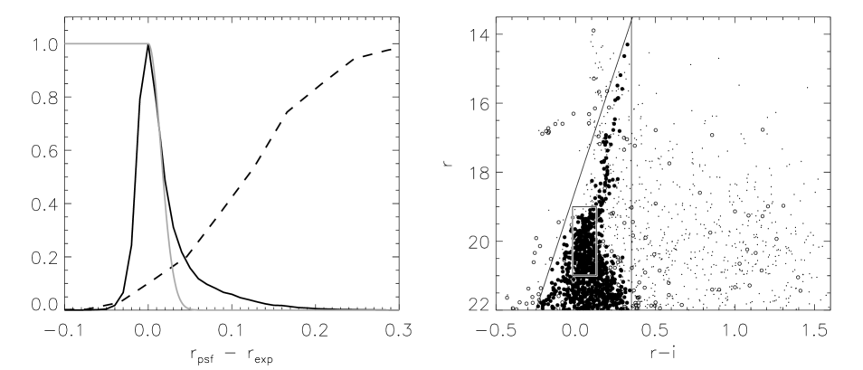
Visual examination of APM-scanned distributions of POSS II detected images in this region already reveals discernible galaxies in the vicinity of the cluster. SDSS provides a crude separation into stars and galaxies, but there is a contamination of the stellar sample by galaxies, particularly at faint magnitudes. The left panel of Figure 1 shows the difference between the magnitudes obtained by PSF photometry and by fitting an exponential profile, namely $r_{\rm psf}-r_{\rm exp}$. This is the concentration parameter introduced by Scranton et al. (2002). Stars are tightly concentrated around zero, whereas galaxies show a significant positive excess. We minimize contamination by external galaxies by using the taper function plotted as a solid grey line in Figure 1. The taper is unity for $r_{\rm psf}-r_{\rm exp}<0$ and is one wing of a Gaussian with dispersion $0.015$ for $r_{\rm psf}-r_{\rm exp}>0$. This taper function is used to multiply the output probabilities of the neural networks, and therefore gives less weight to the contribution of likely contaminants. Effectively, this means that we only use stars with $r_{\rm psf}-r_{\rm exp}<0.05$, which number 87760 in total.

We select cluster stars to lie within a distance $r_{1}=0.14^{\circ}$ of the cluster center. We have chosen $r_{1}$ to be larger than the half-light radius ($0.038^{\circ}$) because the central parts of the cluster are missing. We identify the upper main sequence, sub-giant and giant branch stars from the color cuts, $r-i<0.35$ and $r>-14(r-i)+18.5$. There is also a subsidiary color cut  in $g-r$ to refine the selection, which leaves 896 stars. These are shown in the right panel of Figure 1 as filled circles. The open circles are the remaining stars within $r_{1}$, predominantly foreground stars and some horizontal branch stars belonging to the cluster. The filled circles are the stars used in the training set with target value unity. The dots are stars lying beyond $r_{2}=1^{\circ}$, larger than any estimate of the tidal radius of the cluster. We choose these stars to have target value zero. They are mainly field stars belonging to the disk and the halo.

Ideally, we would like the region in the data space around the decision boundary to be well-sampled in the training set. The number of selected stars is set by requiring the field stars and the cluster stars around the cluster main sequence turn-off to be roughly equal. In practice, this is implemented by requiring the training set to have roughly equal numbers of the populations in the color-magnitude box $-0.02<r-i<0.13$ and $19<r<21$. This gives a total of $\sim 7000$ stars in the training set.

In a multi-layer perceptron, the neurons or processing units are arranged in layers. The input data are fed to the bottommost layer. The output value emerges from the topmost layer, the intervening layers are hidden. The value of the neuron in any layer is calculated by the sum over the weights multiplied by the activations of the neurons connected to it. The activation is computed from the value of the neuron via an activation function. We use the logistic function $f(v)=1/(1+\exp(-v))$, where $v$ is the value of the neuron (Belokurov et al. 2003). This allows us to interpret the output of the network as a posterior probability (Bishop 1995, section 6.7). Given the input data and a set of weights, we can construct an error function, which quantifies the performance of the network. We use a particular form appropriate for two-class problems, namely the cross-entropy error (Bishop 1995, section 6.10). During training, we obtain the weights that minimise the error function over the training set using a steepest descent scheme. In practice, this is done by performing a sequence of iterative up-dates using a variant of back-propagation, which helps to prevent entrapment in local minima (see e.g., Bishop 1995, section 7.5). A further refinement is to add an additional term to the error function, which is the sum of the squares of the weights multiplied by a weight decay parameter. Adjusting this parameter enables us to control the magnitude of weights and hence to minimise any over-fitting. This can be done automatically during training.

The neural networks are constructed with the Stuttgart Neural Network Simulator (SNNS). There are five neurons in the input layer, corresponding to the normalized fluxes in $u,g,r,i$ and $z$. By normalized, we mean the following. The mean and dispersion of the fluxes in the entire field are computed. The network input is then the flux with the mean subtracted and scaled by the standard deviation (e.g., Belokurov et al. 2003). There is one output layer, which approximates the probability of a globular cluster star given the data $P(C_{1}|x)$. The training algorithm is resilient back-propagation with adaptive weight decay (Bishop 1995, section 7.5.3). The networks are trained for a total of 4000 iterations, with weight decay parameter adjusted every 200.

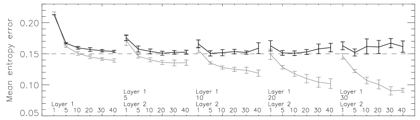
The number of hidden layers and neurons can be freely chosen and is set by experimentation on the data. Figure 2 shows the mean cross-entropy error – defined as the total error normalised by the number of degrees of freedom (number of patterns minus number of network parameters) – for the training and test sets for different network architectures. In this experiment, the original training set was split randomly into two of equal sizes. One of these only was used for training, the other for testing. Of course, there are no patterns in common. As discussed by Belokurov et al. (2004), the error in the training set diminishes with increasing network complexity, but the error in the test set flattens off and eventually starts to rise. An optimum architecture is therefore given by the onset of flattening, as more neurons in the hidden layers will make little further improvement. Examination of the figure suggests that networks with ($5:5:20:1$) or ($5:10:5:1$) or ($5:20:5:1$) are optimal. This notation refers to the number of neurons in the input, first hidden, second hidden and output layers. For our final results, we use committees of 10 neural networks with architecture ($5:10:5:1$), averaging over the network outputs.

Figure 3.— Plot of the ratio of mean outputs for field and for globular cluster stars as a function of magnitude bin $r_{\rm psf}$.

Figure 4.— Left: Contours of mean network output (proportional to the star density) for the globular cluster NGC 5466. The contours mark the levels with network output at $1.5,2,2.5,3,5,10$ and $20\sigma$ above the mean (see text for details). The trajectory is shown as a dotted line. An arrow marked with $\mu$ shows the direction of motion, while one marked with $b$ shows the direction of increasing Galactic latitude. The grey-scale shows the background galaxy density (in number per square degree). Filled circles are blue horizontal branch stars. Right: Detail of the innermost $1^{\circ}\times 1^{\circ}$ of the cluster. The dots are the stars used in the training set. [The left (right) panel uses Gaussian smoothing with FWHM $=0.3^{\circ}$ ($=0.1^{\circ}$) and a median filter with window size $0.4^{\circ}$ ($0.2^{\circ}$).]

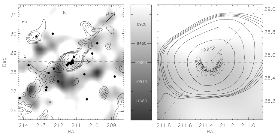
Figure 3 gives an idea of the effectiveness of the classification. It shows the ratio of mean outputs for field and for globular cluster stars as a function of magnitude bin. For a perfect classification, this ratio is close to zero. We see from Figure 3 that the slope of the curve changes abruptly at $r\approx 20$. This can be attributed to the broadening of the top of the main sequence in color space. This increases the number of misclassifications – that is, the number of cluster stars assigned a lower output and field stars assigned a higher output. This suggests applying a magnitude taper function to the network outputs according to the value of $r_{\rm psf}$. Specifically, the taper is unity for stars brighter than $r_{\rm psf}=20$, and is one wing of a Gaussian with dispersion $0.4$ for stars fainter than $r_{\rm psf}=20$.

An alternative to using taper functions in concentration index and magnitude is a hard cut, and tests show that this yields very similar final results.

4. Results

To produce contour maps of the structure around NGC 5466, we first divide the $6^{\circ}\times 6^{\circ}$ field of view into 900 bins with size $0.2^{\circ}$ on a side. We then use Gaussian smoothing and median filtering (the IDL routine FILTER_IMAGE as detailed in the figure caption), followed by cubic splines for interpolation. This yields the maps shown in Figure 4, which show curves of constant mean network output [eqn (2-1)]. This is directly proportional to the stellar number density. The contour levels are chosen in the following way. The distribution of mean network output $P(C_{1})$ for all bins in the field of view is a Gaussian with the centre close to zero and an extended right-hand tail, corresponding to cluster stars. The contour levels shown in Figure 4 correspond to $P(C_{1})$ values at $1.5,2,2.5,3,5,10$ and $20\sigma$ above the mean.

The inner part of the cluster is probably spherical, even though the right panel of Figure 4 shows some distortion of the inner contours. This is understandable, as the SDSS pipeline suffers from crowding problems in the dense center. This is illustrated by the dots in the right panel, which show the cluster stars actually used in the training set.

The outer parts of the cluster are deformed. The tidal tails of NGC 5466 are clearly visible, stretching out in a broadly symmetrical fashion on both sides of the cluster. Also shown is the background galaxy density, using the distribution of objects identified as galaxies by the SDSS pipeline. There is a cluster of galaxies lying behind the southern tail and this may partly account for the broken cluster density contours, as well as some of the asymmetries in the substructure between the tails.

There are two straightforward tests that support the tidal tail hypothesis. First, the proper motion of NGC 5466 is known from Hipparcos (Odenkirchen et al. 1997). The projection of the orbit is plotted on Figure 4. It is in good agreement with the location of the tails, which should of course be distended along the orbit. The position angle (with respect to Galactic North through East) of the tails varies from $\sim 30^{\circ}$ at 20’ to $\sim 45^{\circ}$ in the tails. This is in good agreement with the tidally-induced perturbations in the starcounts already found by Odenkirchen & Grebel (2004) using APM scanned POSS I plates of the inner 20’ of NGC 5466. Second, the positions of blue horizontal branch stars are also shown in the Figure 4 as filled circles. Let us recollect the horizontal branch was excised from the training set (see the right panel of Figure 1) and so the positions of these stars have not therefore contributed to the analysis so far. Nonetheless, these stars also seem to form an extended distribution stretched out along the tails, together with some field star interlopers. The total number of blue horizontal branch stars is small (26), so this test is suggestive rather than conclusive.

5. Discussion and Conclusions

We have identified tidal tails around the high latitude Galactic globular cluster NGC 5466. There have been tentative indications of tidal tails before from the starcounts in the inner $20^{\prime}$ of the cluster (Odenkirchen & Grebel 2004). Here, we have provided an unambiguous identification of extended structure around the cluster. The tidal tails have been traced for over $4^{\circ}$ of arc, using the high quality Sloan Digital Sky Survey (SDSS) photometric data. Numerical simulations of the evolution of NGC 5466 are underway.

References

- Adelman-McCarthy et al. (2005) Adelman-McCarthy J.K. et al. 2005, ApJS, submitted (astro-ph/0507711)
- Belokurov et al. (2003) Belokurov, V., Evans, N. W., & Le Du, Y. 2003, MNRAS, 341, 1373
- Belokurov et al. (2004) Belokurov, V., Evans, N. W., & Le Du, Y. 2004, MNRAS, 352, 233
- Bishop (1995) Bishop C.M. 1995, Neural Networks for Pattern Recognition, Oxford University Press, Oxford
- Dehnen et al. (2004) Dehnen W., Odenkirchen M., Grebel E. K., Rix H.-W. 2004, AJ, 127, 2753
- Dinescu et al. (1999) Dinescu D.I., Girard T. M., van Altena W. F. 1999, AJ, 117, 1792
- Fukugita et al. (1996) Fukugita, M., Ichikawa T., Gunn J. E., Doi M., Shimasaku K., Schneider D. P. 1996, AJ, 111, 1748
- Harris (1996) Harris W.E. 1996, AJ, 112, 1487
- Ibata et al. (1997) Ibata R.A., Wyse R.F.G., Gilmore G., Irwin M.J., Suntzeff N.B. 1997, AJ, 113, 634
- Leon et al. (2000) Leon S., Meylan G., Combes F. 2000, AA, 359, 907
- Lupton et al. (2001) Lupton R., Gunn J. E., Ivezić Z., Knapp G. R., Kent S., Yasuda, N. 2001, ASP Conf. Ser. 238: Astronomical Data Analysis Software and Systems X, 238, 269
- Majewski et al. (2003) Majewski S.R., Skrutskie M.F., Weinberg M.D., Ostheimer J.C. 2003, ApJ, 599, 1082
- Odenkirchen & Grebel (2004) Odenkirchen M., Grebel E. K. 2004, ASP Conf. Ser. 327: Satellites and Tidal Streams, 327, 284
- Odenkirchen et al. (1997) Odenkirchen M., Brosche P., Geffert M., Tucholke H.-J. 1997, New Astronomy, 2, 477
- Odenkirchen et al. (2001) Odenkirchen M., et al. 2001, ApJ, 548, L165
- Odenkirchen et al. (2003) Odenkirchen M., et al. 2003, AJ, 126, 2385
- Rockosi et al. (2002) Rockosi C. M., et al. 2002, AJ, 124, 349
- Schlegel et al. (1998) Schlegel D. J., Finkbeiner D. P., Davis M. 1998, ApJ, 500, 525
- Scranton et al. (2002) Scranton, R., et al. 2002, ApJ, 579, 48
- Spitzer & Hart (1971) Spitzer L. J., Hart M. H. 1971, ApJ, 164, 399
- Yanny et al. (2003) Yanny B., et al. 2003, ApJ, 588, 824
- York et al. (2000) York D. G., et al. 2000, AJ, 120, 1579